Sometimes I need to summarize numerical data in a table. I know how to do this in a report—by using a calculation in a text box, in the report’s footer. But how can I get a sum or average without having to create a report (or pull out a calculator)?

SQL provides aggregate functions that provide summaries of data. Two popular aggregate functions are Sum and Avg (for calculating the average). You can easily incorporate these into your query’s design right within the query grid.

To use an aggregate function, select the View →Totals menu option while in the query grid (or, in Access 2007, click the Sigma (Σ) button in the Ribbon). This makes the Total row display in the grid. The Total row provides the assorted aggregate functions in a drop-down list.

Say you have a tblSales table containing a Customer_ID field, a PurchaseDate field, and an Amount field. There are records spanning dates from 2002 through 2005. To get a fast grand total of all the amounts in the table, just apply the Sum function to the Amount field. Figure 2-1 shows the design of the query, with the Sum function selected from the drop-down list in the Total row for the Amount field.

Figure 2-1. Selecting the Sum aggregate function

shows the result of running the query.

Figure 2-2. The result of running the Sum query

Note that a derived field name, SumOfAmount, has been used in the result. If you want, you can change this name in the SQL or by using an expression in the Field row of the query grid. Figure 2-3 shows how you can change the returned field name to Grand Total by using that name in the Field row, along with a colon (:) and the real field name.

Figure 2-3. Specifying a dynamic field name

To return an average of the values, use the same approach, but instead of Sum, select Avg from the drop-down list in the Total row.

Aggregate functions are flexible. You can apply criteria to limit the number of records to which the aggregation is applied—for example, you can calculate the average amount from purchases in just 2005. Figure 2-4 shows how to design a query to do so. Note that the criterion to limit the Amount field is placed in the second column, not in the same column that contains the Avg function. Also, the Show box is unchecked in the column with the criterion, so only the average in the first column is displayed when the query is run.

Figure 2-5 shows another example: a query design to calculate an average amount from amounts that are greater than or equal to 200. The average returned by this query will be higher than that returned by a query based on all the records.

The SQL generated from this design is:

	SELECT Avg(tblSales.Amount) AS AvgOfAmount
	FROM tblSales
	WHERE (((tblSales.Amount)>=200));

Figure 2-4. Calculating the average of purchases in 2005

Figure 2-5. Calculating an average of purchases above a threshold

I have a table of data containing customer address information. One of the fields is State. How do I create a query to return the number of customers in each state?

When a query uses aggregate functions, the Group By clause is a keystone. This SQL clause provides a grouping segregation, which then allows aggregation summaries to be applied per grouping. In this example, the Group By clause is applied to the State field. Then, the Count aggregate function is used to return the count of customers per group (i.e., per state).

Figure 2-6 shows the design of the query. The first column groups the State field. In the second column, the Count function is selected from the drop-down list in the Total row.

Figure 2-6. Using Count with Group By

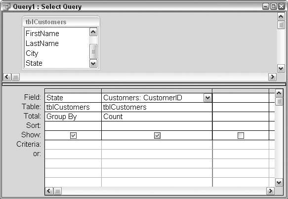
Figure 2-7 shows the result of running the query. The number of customers in each state is returned.

Figure 2-7. Returned counts per state

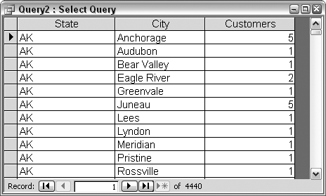
The Group By clause can be applied to more than one field. In such a case, in sequence, each field that uses Group By further defines the narrowness of the count at the end.

Let’s refine our count so we can see how many customers are in each city within each state. Figure 2-8 shows the breakdown of customers in Alaska by city. In the query result shown in Figure 2-7, Alaska has a count of 20 customers. In the query result shown in Figure 2-8, there are still 20 customers listed in Alaska, but now you can see the counts per city.

The SQL statement for the query in Figure 2-8 is this:

	SELECT tblCustomers.State, tblCustomers.City,
	Count(tblCustomers.CustomerID) AS Customers
	FROM tblCustomers
	GROUP BY tblCustomers.State, tblCustomers.City;

Figure 2-8. Count of customers grouped by state and city

I know how to create on-the-fly fields in a query (see Inserting On-the-Fly Fields in Select Queries), and how to include some conditional intelligence. How, though, do I access a value that is not in an underlying table or query, but instead comes from another table altogether? How can I develop comprehensive expressions in a query?

Expressions are a powerful feature in Access. Expressions are used in a number of ways, such as for referencing forms and controls (whether from a macro, from a query, or from VBA). For this example, we’ll use an expression within a query that accesses data from tables not included in the query’s Select statement.

Figure 2-9 shows a query based on two tables: tblClients and tblPets. The key between these tables is ClientID. A field called PetID is the unique key for pets in the tblPets table. Two external tables, tblServiceDates and tblServiceDates_New, contain records of visits made by each pet. The first service date table, tblServiceDates, contains records for pets with PetIDs of up to 299. Higher PetIDs have service date records in the tblServiceDates_New table.

In the query in Figure 2-9 is a field based on a built-up expression, shown here:

	Last Service Date: IIf([PetID]<300,
	DLookUp("Max(DateOfService)",
	"tblServiceDates","[Pet_ID]=" & [PetID]),
	DLookUp("Max(DateOfService)",
	"tblServiceDates_New",
	"[Pet_ID]=" & [PetID]))

Figure 2-9. A query with an expression

This expression combines functions (IIf, DLookup, and Max) to find the last service date for each pet from the respective service date tables.

The full SQL statement that is generated from this design is:

	SELECT tblPets.PetID, tblClients.ClientLastName,
	tblPets.PetType, IIf([PetID]<300,
	DLookUp("Max(DateOfService)",
	"tblServiceDates","[Pet_ID]=" & [PetID]),
	DLookUp("Max(DateOfService)","tblServiceDates_New",
	"[Pet_ID]=" & [PetID])) AS [Last Service Date]
	FROM tblClients INNER JOIN tblPets ON
	tblClients.ClientID = tblPets.ClientID;

In summary, within a query, it is possible to build up a sophisticated expression that uses functions to address data and calculate results that stand outside of the standard SQL syntax.

Entering complex expressions into a single row in the query grid can be difficult, given the limited width of a computer monitor. One workaround is to use the Zoom box, as demonstrated in Figure 2-9. To display the Zoom box, right-click on the query grid where you want the entry to go, and select Zoom from the pop-up menu. Pressing Shift-F2 also displays the Zoom box.

Another choice on the pop-up menu is Build. Selecting this displays the Expression Builder dialog box, seen in Figure 2-10. This utility makes it easy to assemble complex expressions, as it makes all the database objects, functions, and more available for you to use with just a few mouse clicks.

Figure 2-10. The ever-popular Expression Builder

I often write long code routines to read through a table and process its data. It would be great if I could reduce the amount of code required by not creating and reading through a recordset. A select query addresses the table just as well. Is there a way to just apply the processing portion of the code direct from a query?

Calling a function from a query is relatively easy. Just use an extra column in the query grid to create a derived field. In that field, place an expression that calls the function; the returned value from the function is what will appear in the query result.

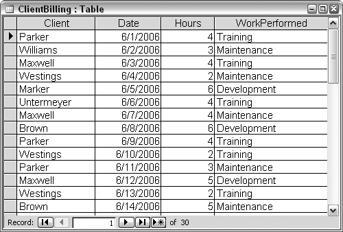
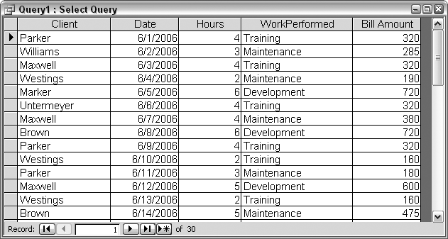
Figure 2-11 shows a table with records of activities performed for different clients. The records list the client name, the date when the work was done, the number of hours it took, and the type of work that was performed. The task is to calculate how much to charge for the work, per record.

First, let’s develop a function that we can call from a query. It’s important that this is a function and not just a sub. We need a returned value to appear in the query results, and while functions return values, subs do not. Here is the bill_amount function:

	Function bill_amount(the_date As Date, the_hours As Integer, _
	    the_client As String, WorkType As String) As Single
	bill_amount = 0 'in case of unexpected input
	Select Case WorkType

Figure 2-11. A table containing records of work performed for clients

	Case "Training"
	  bill_amount = the_hours * 80
	Case "Development"
	  bill_amount = the_hours * 120
	Case "Maintenance"
	  'Parker gets reduced rate regardless of day of week
	  'Other clients have separate weekday and weekend rates
	  If the_client <> "Parker" Then
	    If Weekday(the_date) = 1 Or Weekday(the_date = 7) Then
	      bill_amount = the_hours * 95
	    Else
	      bill_amount = the_hours * 75
	    End If
	  Else
	    bill_amount = the_hours * 60
	  End If
	End Select
	End Function

The function takes four arguments—one each for the four fields in the table—and calculates the amount to bill based on different facets of the data. The type of work performed, the client for whom it was performed, and whether it was done on the weekend (determined with the Weekday function) all determine which hourly rate to use. The hourly rate and the number of hours are then multiplied to determine the billing amount.

Figure 2-12 shows the query design. Note that you don’t have to place the table fields in the grid unless you want them to appear with the values returned from the function.

Figure 2-12. A custom function is called from a query

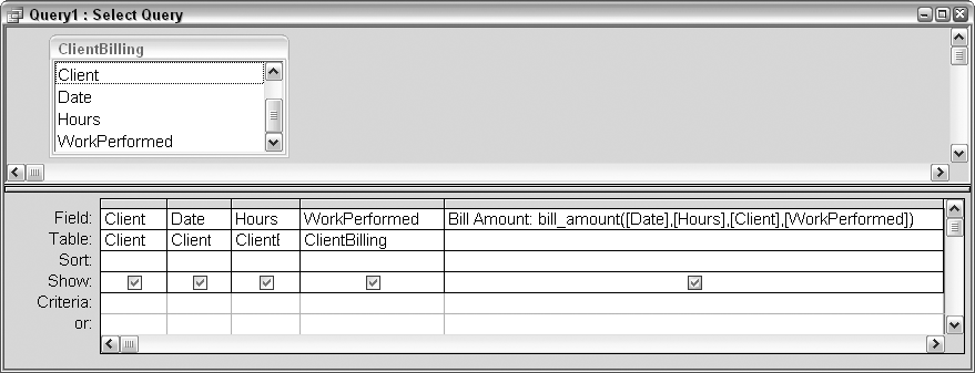
The function is called in the query in a separate column. The structure of the expression is:

	Bill Amount: bill_amount([Date],[Hours],[Client],[WorkPerformed])

Bill Amount is the name of the temporary field. bill_amount is the name of the function, and the four fields are included as arguments. The fields are each encased in brackets, consistent with the standard Access field-handling protocol.

When the query is run, the fifth column contains the billable amount, as shown in Figure 2-13.

Figure 2-13. The billable amounts are returned

Calling functions from queries opens up many ways of working with your data. The function used in this example is short and processes an easy calculation. But do note that this function actually calls another function, Weekday. The point is that you can develop sophisticated functions that perform all types of processing.

Both custom functions and built-in functions can be called from a query. Further, the query does not have to be a select query; you can call functions from action queries (discussed in Chapter 3) as well. Figure 2-14 shows an example of using two built-in functions, IIf and Weekday, to update the value in a field. If the date falls on the weekend, -Weekend is appended to the client name.

Figure 2-14. Built-in functions used in an update query

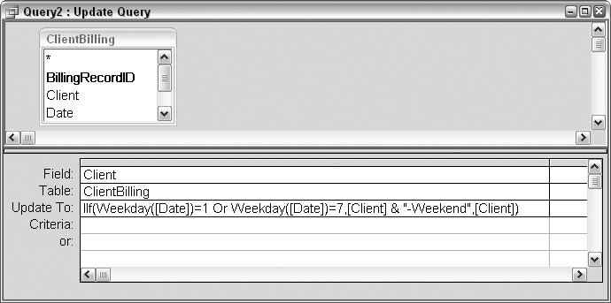
Take a closer look at the expression used in the Update To row:

	IIf(Weekday([Date])=1 Or Weekday([Date])=7,[Client] & "-Weekend",[Client])

If the weekday is a 1 or a 7 (a Sunday or a Saturday), -Weekend is appended to the client name; otherwise, the client name is used for the update as is. In other words, every row is updated, but most rows are updated to the existing value.

Regular expressions provide the ability to set up sophisticated string patterns for matching records. Can a regular expression be used as the criterion in a query?

Regular expressions, popularized by Perl and other Unix-based languages, provide powerful string-matching capabilities. For Access and other Windows-based applications, adding a reference to the VBScript Regular Expressions library makes using regular expressions possible. You can set up the reference in the Visual Basic Editor (VBE). To display the VBE from Access, just press Alt-F11. While in the VBE, use the Tools →References menu option to display the References dialog. Then set a reference to Microsoft VBScript Regular Expressions 5.5 (your version number may be different), as shown in Figure 2-15.

Figure 2-15. Setting a reference to the VBScript Regular Expressions library

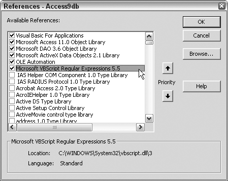
Figure 2-16 shows a table with hypothetical transaction records.

The values in the TransactionRecord field are concatenations of separate codes and values that follow this pattern:

Figure 2-16. A table with transaction records

Given this pattern, let’s construct a query that will identify transactions that are either adjustments or deposits, are for the Sales department, and are for amounts of 500 or greater. Put another way, our task will be to identify transaction records consisting of an A or a D, followed by any two numbers, followed by SA, followed by a number that is 5 or greater, and any two other numbers.

To make use of pattern matching, we’ll use a custom function to create a regular expression (regexp) object. In a separate code module, enter this function:

	Function validate_transaction(transaction_record As String, _
	    match_string As String) As String
	  validate_transaction = "Invalid Record"
	  Dim regexp As regexp
	  Set regexp = New regexp
	  With regexp
	    .Global = True
	    .IgnoreCase = True
	    .Pattern = match_string
	    If .Test(transaction_record) = True Then
	      validate_transaction = "Valid Record"
	    End If
	  End With
	  Set regexp = Nothing
	End Function

The transaction record and the regular expression pattern to match are given to the function as arguments. The function code initially sets the return value to Invalid Record. A regexp object is set, and the transaction record is tested against the pattern. If the transaction record matches the pattern, the return value is changed to Valid Record.

Now, we’ll call this function from a query. Figure 2-17 shows a select query that places the call to the function in the second column. Note that the column with the function to call is set to a descending sort. This is so all valid records will appear at the top. Unlike a typical select query that returns just the records that match the criteria, in this case all records are returned, so it makes sense to group together all the valid records.

Figure 2-17. A regular expression pattern coded into a query

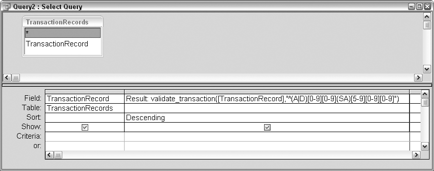
Figure 2-18 shows the result of running the query. The valid records are at the top.

The pattern used for matching the transaction records look like this:

	^(A|D)[0-9][0-9](SA)[5-9][0-9][0-9]

A detailed explanation of regular expression syntax is beyond the scope of this recipe, but in a nutshell, here is what the pattern calls for:

Figure 2-18. Records are validated using a regular expression

Test is just one method of the regexp object. There also are Execute and Replace methods. Execute creates a collection of matches. This is useful in code-centric applications, where further processing would take place in a routine. The Replace method replaces a match with a new string. Figure 2-18. Records are validated using a regular expression

I have a list of teams and a list of locations with ballparks. I wish to create a master list of all the combinations possible between these two lists.

We typically use queries to limit the amount of returned records, and at the very least, we expect the number of returned records to be no greater than the number of records in the largest table or query being addressed.

However, there is a special type of join, called a Cartesian join, that returns the multiplicative result of the fields in the query (otherwise known as the Cartesian product). A Cartesian join is the antithesis of standard joins—it works as if there is no join. Whereas the other join types link tables together on common fields, no field linking is required to return a Cartesian product.

Figure 2-19 shows a table of teams and a table of locations. Simply put, we are looking for all the combinations that can exist between these two tables.

Figure 2-19. A table of teams and a table of locations

Figure 2-20 shows the design of a query that essentially has no join. There is no line connecting the tables. In fact, the single fields in each table really don’t relate to each other.

The SQL generated by the design in Figure 2-20 looks like this:

	SELECT Teams1.Team, Locations.Location
	FROM Teams1, Locations;

Figure 2-20. Design of a Cartesian join

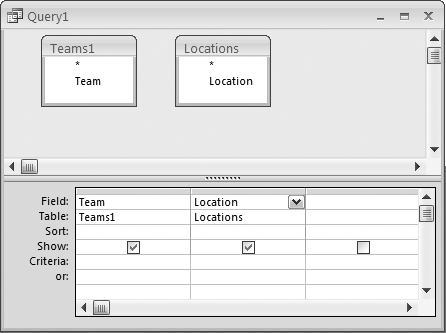
Note that even in the SQL, no join is stated.

When the query is run, all possible combinations are returned. The Teams1 table has 18 records, and the Locations table has 10 records. Figure 2-21 shows the query result, which returns 180 records.

What if, for example, you needed a master list of all possible team versus team combinations? This task is a little different, as it involves creating a Cartesian product of a single field. If you design a query with one table and just pull the field into two columns, you will not gain any new records or combinations. You need a duplicate teams table to make this work.

Copy the Teams1 table and name the copy Teams2. You now have two tables that are identical, apart from their names. When making a Cartesian query that’s based on two identical fields, your aim will typically be to get all possible combinations except for an entity combined with itself. For example, there is no point in matching a team with itself—the Carmel Carriers will never play against the Carmel Carriers!

Figure 2-22 shows a design that will return all possible match combinations, except those where the teams are the same. The SQL statement for this query is:

	SELECT Teams1.Team, Teams2.Team
	FROM Teams1, Teams2
	WHERE (((Teams1.Team)<>[Teams2].[Team]))
	GROUP BY Teams1.Team, Teams2.Team;

Figure 2-21. The number of returned records equals the product of the numbers of records in the source tables

Figure 2-22. A Cartesian join designed to avoid same-name matches

Figure 2-23 shows the result of running the query. Notice that there is no record in which the Ardsley Achievers appear in both columns—this type of duplication has been avoided. To confirm this, you can check the number of returned records. There are 18 teams, and 18 multiplied by 18 is 324, yet only 306 records were returned. The 18 records that would have shown the same team name in both columns did not make it into the result.

Figure 2-23. A Cartesian product without same-name matches

How can I view my relational data in a hierarchical manner? I know I can use Group By clauses in a query, but with an abundance of data points, this becomes cumber-some and creates many records. Is there another way to see summaries of data based on groupings?

A crosstab query is a great alternative to a standard select that groups on a number of fields. Figure 2-24 shows the Student_Grades table, which has five fields: StudentID, Instructor, MidTerm Grade, Final Grade, and Course.

Figure 2-24. A table with instructors, courses, and grades

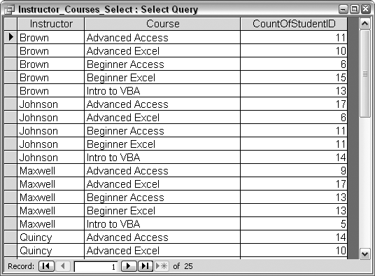
Using the information in the Student_Grades table, it is possible to get a per-instructor count of how many students attended each course. Figure 2-25 shows the design of a standard select query that accomplishes this. The Group By clauses create delineations of Instructor and Course, and within each combination, a Count of the StudentID field returns the count of students. The SQL for this query is:

	SELECT Student_Grades.Instructor,
	Student_Grades.Course,
	Count(Student_Grades.StudentID) AS CountOfStudentID
	FROM Student_Grades
	GROUP BY Student_Grades.Instructor, Student_Grades.Course;

Running the query in Figure 2-25 produces a result with 25 records, shown in Figure 2-26.

Now for the alternative. A crosstab query will return the same student counts, per instructor, per course; however, the layout will be smaller. The design of the crosstab query is shown in Figure 2-27. Crosstabs require a minimum of one Row Heading field, one Column Heading field, and one Value field in which the reporting is done.

Figure 2-25. A select query that returns the count of students per instructor, per class

Figure 2-26. Returned student counts from a select query

In this case, the Value field is the StudentID field, and Count is the selected aggregate function (as it was in the equivalent select query). The Instructor field is designated as a Row Heading, and the Course field is designated as the Column Heading.

Figure 2-27. The design of the crosstab query to count student records

The SQL behind the crosstab query reads like this:

	TRANSFORM Count(Student_Grades.StudentID) AS CountOfStudentID
	SELECT Student_Grades.Instructor
	FROM Student_Grades
	GROUP BY Student_Grades.Instructor
	PIVOT Student_Grades.Course;

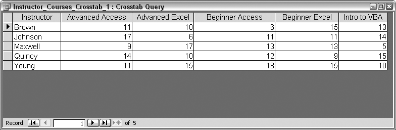
Note the TRANSFORM and PIVOT statements. These are unique to creating a crosstab and are explained in the Discussion section. Figure 2-28 shows the result of running the query. Just five rows are returned—one for each instructor—and there is a column for each course.

Figure 2-28. The result of running the crosstab query

To recap, a crosstab query requires:

To create a crosstab query, select the Query →Crosstab Query menu option while in the query designer. This will cause the Crosstab row to display in the query grid. Alternatively, you can use the Crosstab Query Wizard. To launch the wizard, click the New button while the Queries tab is on top in the database window. Then, select Crosstab Query Wizard in the New Query dialog box.

In the SQL syntax, a TRANSFORM statement is what designates the query as a crosstab. Following directly after the TRANSFORM keyword are the aggregate function and the Value field to be used. The one or more fields following the SELECT statement are the Row Headings. The field following the PIVOT keyword is the field from which the column headings will be drawn.

The previous query produced results in which the row headings were the instructor names and the column headings were the course names (Figure 2-28). Swapping the fields in the SELECT and PIVOT sections reverses the structure of the output. In other words, using this SQL:

	TRANSFORM Count(Student_Grades.StudentID) AS CountOfStudentID
	SELECT Student_Grades.Course
	FROM Student_Grades
	GROUP BY Student_Grades.Course
	PIVOT Student_Grades.Instructor;

creates the output shown in Figure 2-29. Now, the courses are listed as rows and the column headings are the instructor names. Regardless of the layout, the counts are consistent.

Sophisticated crosstabs

In the examples we’ve looked at so far in this recipe, after the TRANSFORM keyword, we’ve applied an aggregate function to a single field. A limitation of crosstab queries is that only one Value field can be evaluated; attempting to include a second aggregation would result in an error. But what if you need to process information from more than one field?

Figure 2-29. The crosstab with a different layout

While only one value can be returned for each row and column intersection, there are options for how that value is calculated. Let’s say we need to find the overall average for each course—that is, the combined average of the MidTerm Grade and Final Grade fields. This will provide an overall average per course, per instructor. The catch here is that two fields contain values that need to be considered: MidTerm Grade and Final Grade.

To accomplish this task, we’ll place a function call where the Value field is usually specified, and we’ll select Expression in the Total row. Figure 2-30 shows the query design.

Figure 2-30. Using a function to return the single crosstab value

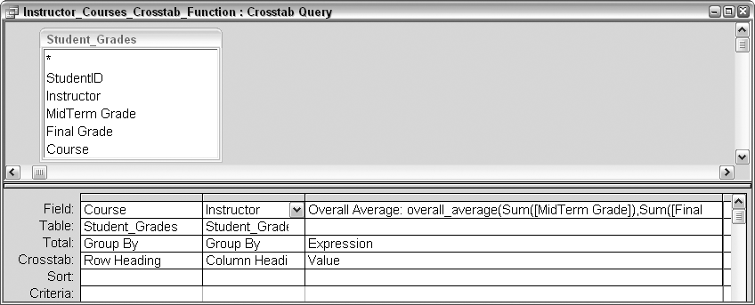
The full expression reads like this:

	Overall Average: overall_average(Sum([MidTerm Grade]),
	Sum([Final Grade]),Count([StudentID]))

The SQL statement looks like this:

	TRANSFORMoverall_average(Sum([MidTerm Grade]),
	Sum([Final Grade]),Count([StudentID])) AS [Overall Average]
	SELECT Student_Grades.Course
	FROM Student_Grades
	GROUP BY Student_Grades.Course
	PIVOT Student_Grades.Instructor;

As the query runs, the overall_average function is called. The arguments it receives are the midterm grade, the final grade, and the count of students. Bear in mind that, one at a time, these three arguments are providing information based on a combination of instructor and course.

The overall_average function calculates the overall average by adding together the sum of each grade type (which creates a total grade), and then dividing the total by twice the student count—each student has two grades in the total, so to get the correct average, the divisor must be twice the student count. Here is the function:

	Function overall_average(midterm_sum As Long, _
	    final_sum As Long, student_count As Integer) As Single
	  overall_average = (midterm_sum + final_sum) / (student_count * 2)
	End Function

Figure 2-31 shows the result of running this crosstab. The returned values are the overall averages of the combined grades.

Figure 2-31. Result of the crosstab with a calculated value field

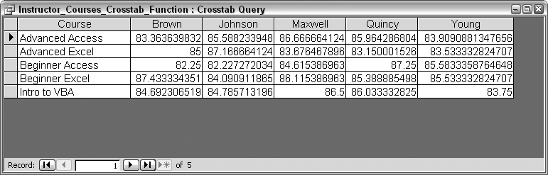
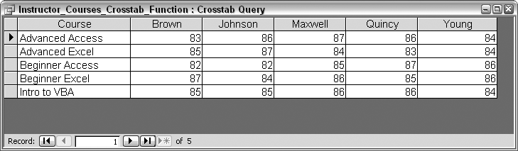
The returned values in Figure 2-31 are drawn out to several decimal places. Using the Round function helps pare them down. Here is the updated function, with the rounded values shown in Figure 2-32:

	Function overall_average(midterm_sum As Long, _
	    final_sum As Long, student_count As Integer) As Single
	  overall_average = Round((midterm_sum + final_sum) / (student_count * 2))
	End Function

Figure 2-32. Rounded crosstab values

While you can only display a single value in the result, you have many options for calculating that value. The approach presented here—using a function to calculate a value it’s not possible to determine with the singular aggregate functions—is a useful and flexible one.