I’d like to understand how the values of a data element I’m collecting are distributed.

You can use a frequency table and a histogram to identify how the data values are distributed.

A frequency table begins by defining a set of “buckets,” and associating a range of data values with each bucket. Each row is then read from the database, and each element is placed in the appropriate bucket based on its value. Once all of the rows have been processed, the frequency table can be constructed by counting the number of data elements in each bucket.

For example, consider the following list of values:

	43, 45, 17, 38, 88, 22, 55, 105, 48, 24, 11, 18, 20, 91, 9, 19

Table 10-1 contains the number of data elements for each given set of ranges.

While you may think that this process sounds complicated enough that you’d have to write a VBA program to do the counting, it turns out that it’s fairly easy to build a SQL SELECT statement that does the job without a single line of code. Consider the following statement:

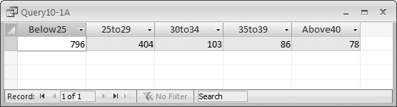
	SELECT Sum(IIf([DisneyClose]<25,1,0)) AS Below25,
	   Sum(IIf([DisneyClose]>=25 And [DisneyClose]<30,1,0)) AS 25to29,
	   Sum(IIf([DisneyClose]>=30 And [DisneyClose]<34,1,0)) AS 30to34,
	   Sum(IIf([DisneyClose]>=35 And [DisneyClose]<39,1,0)) AS 35to39,
	   Sum(IIf([DisneyClose]>=40,1,0)) AS Above40
	FROM Stocks
	WHERE (((Stocks.Date)>#1/1/2000# And (Stocks.Date)<#1/1/2006#));

This statement returns a single row of data representing the frequency table and a total of five columns, where each column represents a particular range, and the value of the column represents the number of values that fall into that range.

The statement uses the Sum and IIf functions. The Sum function is an aggregate function that returns the sum of all the values generated by the expression inside. The IIf function takes three parameters: the first is a Boolean expression, the second is the value returned if the Boolean expression is true, and the third is the value returned if the Boolean expression is false.

The real trick to this statement is the way the IIf function returns 1 if the value is in the column’s range, and 0 if it isn’t. This means that for any particular row, one column will have a 1, while the rest of the columns will have 0s. The Sum function thus returns the number of rows that contain values in each given range. Running the query will return a result table similar to Figure 10-1.

Figure 10-1. Running the query results in this simple frequency table

You can convert a frequency table into a histogram in one of two ways: by exporting the data to Excel and using its charting tools to create a bar or column chart, or you by viewing the result table in Access as a PivotChart (see Figure 10-2).

Figure 10-2. Using a PivotChart to display a histogram

To create the PivotChart, right-click on the datasheet view of the query result, and choose PivotChart from the context menu. Then, drag the fields from the Chart Field List (see Figure 10-3) onto the plot area to create your histogram.

If you need a neatly formatted chart, you should export your data into Excel, where you’ll have more control over the chart’s formatting. On the other hand, using Access’ PivotCharts makes it easy to determine the right level of granularity.

If you don’t like how the chart looks, you can easily change the ranges in the query and see the results much faster than you would in Excel.

Figure 10-3. The list of fields that can be displayed in the PivotChart

I want to compute the mean, mode, and median of a particular column.

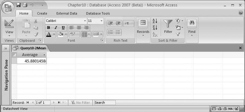
To compute the mean of a column, you can simply use the Avg aggregate function, like this:

	SELECT Avg(Stocks.DisneyClose) AS Average
	FROM Stocks

The result of this query is shown in Figure 10-4.

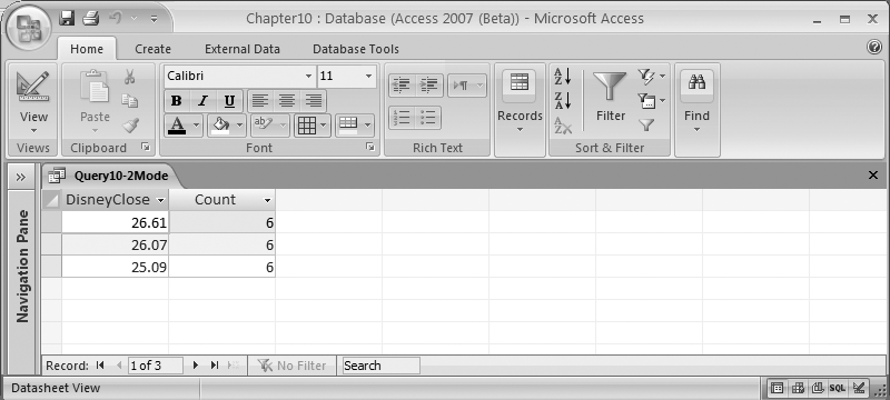
Computing the mode of a column is a little more complex, but the following SELECT statement should give you an idea of how to do it:

	SELECT Top 1 Stocks.DisneyClose, Count(*) AS [Count]
	FROM Stocks
	GROUP BY Stocks.DisneyClose
	ORDER BY Count(*) DESC;

You can see the result in Figure 10-5.

Figure 10-4. Computing the mean for a set of data

Figure 10-5. Computing the mode of a column

Computing the median of a column is more complicated still. The following SELECT statement will generate the result shown in Figure 10-6:

	SELECT A.DisneyClose
	FROM Stocks AS A, Stocks AS B
	GROUP BY a.DisneyClose
	HAVING (((Sum(IIf(a.DisneyClose<=b.DisneyClose,1,0)))>=(Count(*)/2))
	   And ((Sum(IIf(a.DisneyClose>=b.DisneyClose,1,0)))>=(Count(*)/2)));

The mean is really just the average of the numbers. In other words, to get the mean, you need to compute the sum of the values and divide the result by the number of values, which is what the Avg function does for you.

Figure 10-6. Computing the median of a column

On the other hand, to find the mode, you must create a list of all of your numbers, order them, and find the most common value. Note that this value is not necessarily the same as the average. Consider the following set of numbers:

	1, 1, 1, 1, 496

The average of these numbers is 100, while the mode is 1.

The SELECT statement that returns the mode works by using the GROUP BY clause to count the number of occurrences of each individual value, then orders them from the value with the highest count to the one with the lowest count. Finally, it returns the number or numbers that have the largest count:

	SELECT Top 1 Stocks.DisneyClose, Count(*) AS [Count]
	FROM Stocks
	GROUP BY Stocks.DisneyClose
	ORDER BY Count(*) DESC;

The median is the most complicated value to compute. To find the median, you arrange the numbers in order, and then select either the middle value (if there is an odd number of values) or the average of the two values in the middle (if there is an even number of values). Thus, in this set of numbers, 3 is the median:

	1, 2, 3, 4, 5

while in this set of numbers, the median is 3.5:

	1, 2, 3, 4, 5, 6

The following SQL statement may look tricky at first, but it’s really easy to follow. It begins by using the GROUP BY clause to reduce the number of individual data values to process. Then, it uses the IIf function to determine how many numbers appear before and after the current value in the sequence. When the number of data values before and after are the same, you’ve found the median value:

	SELECT A.DisneyClose
	FROM Stocks AS A, Stocks AS B
	GROUP BY a.DisneyClose
	HAVING (((Sum(IIf(a.DisneyClose<=b.DisneyClose,1,0)))>=(Count(*)/2))
	   And ((Sum(IIf(a.DisneyClose>=b.DisneyClose,1,0)))>=(Count(*)/2)));

The downside to using a SELECT statement to compute the median is the amount of processing that’s required. Basically, this approach reads the entire table for each value it processes. For small tables this is fine, but if your table contains a thousand or more rows, you’ll find that running the query takes a long time. However, the following VBA routine is very quick, no matter what the size of your table is:

	Sub Example10_2Median()

	Dim rs As ADODB.Recordset
	Dim d As Double

	Set rs = New ADODB.Recordset
	rs.ActiveConnection = CurrentProject.Connection

	rs.Open "Select DisneyClose From Stocks Order By DisneyClose", , _
	   adOpenStatic, adLockReadOnly

	If rs.RecordCount Mod 2 = 1 Then
	   rs.Move rs.RecordCount / 2 + 1
	   d = rs.Fields("DisneyClose")

	Else
	   rs.Move rs.RecordCount / 2
	   d = rs.Fields("DisneyClose")

	   rs.MoveNext
	   d = (d + rs.Fields("DisneyClose")) / 2

	End If

	rs.Close

	Debug.Print "Median = ", d

	End Sub

The routine begins by opening a static, read-only Recordset. Once the Recordset is open, the code determines whether the RecordCount property is even or odd. If the value of RecordCount is odd, it uses the Move method to skip to the exact center of the table, and retrieves the middle value. To find the center row, the routine divides the value of RecordCount by 2, rounds down the result to the nearest integer value, and then adds 1. The value in this row is then returned as the median.

If the value of RecordCount is even, the same process is followed, but after retrieving the value in the “center” row, the routine moves to the next row and retrieves its value as well. Then, it computes the average of the two values and returns this as the median.

I’d like to understand how much my data varies by using standard statistical functions like standard deviation and variance.

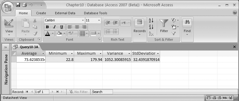
Given a column of data, the following SELECT statement returns a Recordset containing the average, minimum, maximum, variance, and standard deviation values, using the Avg, Min, Max, Var, and StDev functions:

	SELECT Avg([DisneyClose]) AS Average,
	   Min([DisneyClose]) AS Minimum,
	   Max([DisneyClose]) AS Maximum,
	   Var([DisneyClose]) AS Variance,
	   StDev([DisneyClose]) AS StdDeviation
	FROM Stocks

The results are shown in Figure 10-7.

The variance is a measure of the spread of a list of numbers. It’s computed by first determining the average value, and then, for each individual number, calculating the square of the difference between that number and the average. Finally, these values are summed and divided by the total number of values.

Here is the formula to calculate variance:

	           Σ (x - X)2
	Variance = ------------
	                N

where N is the number of values, x is the current value, and X is the average value.

Consider the following set of numbers:

	1, 2, 3, 4, 5

The average is 3, and the sum of the difference of the squares is 10. There are five values, so the variance is 2.

If you replace the 5 with a 10, the average becomes 4, but the variance becomes 10. This indicates that this list of numbers is more spread out than the original list.

One of the issues with using variance is that the number returned as the variance isn’t measured in the same units as the original numbers. Instead, the variance is measured in units squared. If the original numbers were in dollars, for example, the variance would be measured in dollars squared.

Figure 10-7. Computing the variance, standard deviation, and other summary values for a column

Because this isn’t always useful, you can compute the standard deviation by taking the square root of the variance. Standard deviation is measured in terms of the original units. For the set of numbers 1 through 5 (whose variance was 2), the standard deviation is 1.41; for the numbers 1 through 4 and 10, the standard deviation is 3.16.

One way to use variance and standard deviation is to compare two lists of numbers. Consider the following query, which computes the standard deviation for four different stock prices over a five-year period:

	Select StDev(DisneyClose) As Disney,
	   StDev(TimeWarnerClose) As TimeWarner,
	   StDev(GeneralMotorsClose) As GeneralMotors,
	   StDev(FordClose) As Ford
	From Stocks
	Where Date Between #1-1-2000# and #12-31-2005#;

The results are shown in Figure 10-8.

Figure 10-8. Using standard deviation to understand stock prices

Notice that Disney has a standard deviation of 21.42, while Ford has a standard deviation of 11.47. This means that the stock prices for Disney varied much more than the stock prices for Ford during the same period of time. This doesn’t necessarily tell you which stock to buy, but it does help you understand how volatile stock prices are when compared with each other.

I want to compute the covariance of two sets of data.

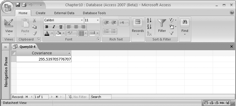
You can use a SELECT statement like the following to compute the covariance for two columns of data:

	SELECT
	   Sum(
	      (DisneyClose –
	         (Select Avg(DisneyClose)
	            From Stocks
	            Where Date Between #1-1-2000# And #12-31-2005#))
	     * (TimeWarnerClose
	        (select Avg(TimeWarnerClose)
	           From Stocks
	           Where Date Between #1-1-2000# And #12-31-2005#))
	      )
	  / Count(*) AS Covariance
	FROM Stocks
	WHERE Date Between #1/1/2000# And #12/31/2005#;

The result is shown in Figure 10-9.

The SELECT statement begins by computing the sum of the products of the differences between each of the values and their average. Then, the covariance is computed by dividing the sum by the number of values processed.

Here is the formula to calculate covariance:

	             (x - X)(y - Y)
	Covariance = -----------------
	                  N

where N is the number of values, x is the current value for the first column, X is the average value for the first column, y is the current value for the second column, and Y is the average value for the second column.

Figure 10-9. Computing the covariance between two columns of data

Variance, discussed in Calculating the Variance in a Set of Data, provides an indication of how much the values for a single variable vary. Covariance, by contrast, measures how much the values for two separate variables vary together. A positive value for covariance means that as the value of one variable increases, so does the value of the other. A negative value for covariance means that as one variable increases, the other one decreases. A value of 0 implies that the two variables are linearly independent—that is, there is no linear relationship between one variable and the other.

I want to compute the correlation of two columns of data.

To compute the correlation, which is an indication of the strength and direction of the linear relationship between two variables, you merely divide the covariance by the product of the two standard deviations. The SELECT statement from Finding the Covariance of Two Data Sets can easily be modified for this purpose. All we have to do is divide the result by the standard deviation aggregate functions described in Calculating the Variance in a Set of Data. The resulting SELECT statement looks like this:

	SELECT
	   Sum(
	      (DisneyClose –
	         (Select Avg(DisneyClose)
	            From Stocks
	            Where Date Between #1-1-2000# And #12-31-2005#))
	      * (TimeWarnerClose -
	         (select Avg(TimeWarnerClose)
	         (select Avg(TimeWarnerClose)
	            From Stocks
	            Where Date Between #1-1-2000# And #12-31-2005#))
	      )
	    / Count(*) AS Covariance / StDev(DisneyClose) / StDev(TimeWarnerClose)
	FROM Stocks
	WHERE Date Between #1/1/2000# And #12/31/2005#;

Unlike covariance, correlation returns a result within a strict range. This makes it possible to compare multiple correlations and draw conclusions.

Correlations return a value between -1 and 1. A value of 0 implies that the two sets of data do not have a linear relationship. A positive value indicates that the two sets of data are linearly related (i.e., as one set of values rises, so does the other). The larger the value is, the stronger the relationship. If you use the same column for both sets of data, you should get a value of 1.

A negative value, on the other hand, means that the data values move in opposite directions from each other. As the correlation coefficient becomes closer to -1, the relationship becomes stronger, with the strongest possible relationship being -1. This would happen if the data values in the second set of data were identical to those in the first (except for their signs).

I’d like to create a table containing all possible permutations of the data that could be returned from a table of values for the specified number of output columns.

The following routine selects all of the values from a table and generates all possible permutations for a given number of slots. It begins by loading the entire source table into an array. While this might seem to waste a lot of memory, it isn’t nearly as bad as you might think. An array of 10,000 names that are 100 characters long occupies a single megabyte of memory. This will save a huge amount of I/O over processing the set of data multiple times.

The sample table we’ll use in this recipe contains 12 values, and we’ll aim to calculate all the possible permutations when 3 of those values are selected at random.

Here’s the routine:

	Sub Example10_6()

	Dim rs As ADODB.Recordset
	Dim StockNames() As String

	Dim i As Long
	Dim j As Long
	Dim k As Long

	Set rs = New ADODB.Recordset
	rs.ActiveConnection = CurrentProject.Connection

	rs.Open "SELECT StockName From StockNames Order By StockName", , _
	   adOpenForwardOnly, adLockReadOnly

	i = 0
	ReDim StockNames(0)

	Do While Not rs.EOF
	   ReDim Preserve StockNames(i)
	   StockNames(i) = rs.Fields("StockName")
	   i = i + 1
	   rs.MoveNext

	Loop
	
	rs.Close
	
	rs.Open "StockPermutations", , adOpenDynamic, adLockOptimistic
	
	For i = 0 To UBound(StockNames)
	   For j = 0 To UBound(StockNames)
	      For k = 0 To UBound(StockNames)

	         If i <> j And j <> k And i <> k Then
	            rs.AddNew
	            rs.Fields("First") = StockNames(i)
	            rs.Fields("Second") = StockNames(j)
	            rs.Fields("Third") = StockNames(k)
	            rs.Update

	         End If

	      Next k

	     Next j

	Next i

	rs.Close

	End Sub

After the data has been loaded, the output table is opened. Note that the output table has already been created and has three columns: First, Second, and Third.

Because we want to fill all three fields, a three-deep nested loop is set up to process the array. If the loop variables are all different (meaning that they point to three unique names), the routine adds a new row to the output table and saves the three selected values to their respective fields. It then updates the row and loops around to process the next set of names.

You can easily modify this routine to accommodate the number of choices you want by adding or subtracting nested For loops. One For loop is required for each choice you wish to generate. You’ll also have to modify the If statement to ensure that you never have two subscripts with the same value.

Permutations describe the possible ways that a group of items can be ordered. Assume that you have three different items: A, B, and C. Here is a list of all possible permutations:

	A B C
	A C B
	B A C
	B C A
	C A B
	C B A.

Mathematically, you can compute the number of permutations using the factorial method. To compute the factorial of a number, simply multiply it by all of the numbers smaller than it. Thus, three items have 3! (i.e., 6) permutations:

	3 x 2 x 1

The problem with generating permutations is that the number of permutations grows incredibly quickly. Four items have 24 permutations, five items have 120, six items have 720, seven items have 5,040, and eight items have 40,320. By the time you reach 14 items, there are already more than 87 billion possible permutations.

Now, let’s return to the task of choosing a subset of items at random from a larger group of items. The number of possible permutations can be computed by the following formula, where n represents the total number of items, and r represents the number of items to return:

	n!/(n-r)!

If, for example, you wanted to choose three items out of a set of five, the equation would look like this:

	5!/(5-3)! = 5!/2! = 60

Thus, when choosing three items out of five, there are a total of 60 possible permutations. When choosing 3 items out of a set of 12, as was done in the code routine presented earlier, there are a total of 1,320 possible permutations; consequently, 1,320 rows will be generated when the routine is executed.

I’d like to create a table containing all possible combinations from another table of data values for the specified number of output columns.

You can use the following routine to compute the number of possible combinations:

	Sub Example10_7()

	Dim rs As ADODB.Recordset
	Dim StockNames() As String
	Dim i As Long
	Dim j As Long
	Dim k As Long

	Set rs = New ADODB.Recordset
	rs.ActiveConnection = CurrentProject.Connection

	rs.Open "SELECT StockName From StockNames Order By StockName", , adOpenForwardOnly,
	adLockReadOnly

	i = 0
	ReDim StockNames(0)
	
	Do While Not rs.EOF
	   ReDim Preserve StockNames(i)
	   StockNames(i) = rs.Fields("StockName")
	   i = i + 1
	   rs.MoveNext
	
	Loop

	rs.Close

	rs.Open "StockCombinations", , adOpenDynamic, adLockOptimistic

	For i = 0 To UBound(StockNames) - 2
	   For j = i + 1 To UBound(StockNames) - 1
	      For k = j + 1 To UBound(StockNames)

	         rs.AddNew
	         rs.Fields("First") = StockNames(i)
	         rs.Fields("Second") = StockNames(j)
	         rs.Fields("Third") = StockNames(k)
	         rs.Update

	      Next k

	   Next j

	Next i
	
	rs.Close
	
	End Sub

The routine begins by loading the source table into memory, and then it opens a new Recordset object referencing the output table. Note that the output table has already been created and has three columns: First, Second, and Third.

The actual combinations are generated by a set of three nested For loops. The loops are structured such that the ranges of index variables never overlap, which guarantees that each set of names will be unique.

Assume that the UBound of the array is 11. When i is 0, j will start at 1 and go to 10, and k will start at 2 and go to 11. When j is 2, k will start at 3, and so forth, until j reaches 10. At that point, k can only take on the value of 11. The last combination of data is generated when i reaches 9, at which point j is 10 and k is 11.

If you need a different number of choices, be sure to include one loop for each choice. The key is to ensure that the loop variables never overlap.

Combinations represent unordered groups of data. This differs from permutations (see Returning All Permutations in a Set of Data), in which the order of the items is important. Just like with permutations, each item can appear in the list only once. But since the order isn’t important, the number of combinations will always be less than the number of permutations.

For example, suppose you have a list of five items: A, B, C, D, and E. If you look for every possible combination of three items from the list, you’ll get these 10 combinations:

	A B C
	A B D
	A B E
	A C D
	A C E
	A D E
	B C D
	B C E
	B D E
	C D E

If you take a look back at Returning All Permutations in a Set of Data, however, you will see that there are 60 possible permutations.

You can compute the number of possible combinations using the following formula, where n represents the total number of items, and r represents the number of items to include:

	n!/r!(n-r)!

So, for the preceding example of choosing three items out of five, you’ll have the following equation:

	5!/3!(5-3)! = 5!/3!(2!) = 10

And, in the earlier code example, choosing 3 items out of 12 results in 220 possible combinations.

I’d like to know how many times a particular value appears in a table.

The following Select statement will determine the number of times the specified value appears in the table. Simply modify the Where clause to select the desired value:

	Select Count(*) As Frequency
	From Stocks
	Where DisneyClose = 24.76;

Suppose you want to identify the frequency of each unique value in the table. For this, you can use a SELECT statement like the following:

	SELECT DisneyClose, Count(*) AS Frequency
	FROM Stocks
	WHERE DisneyClose Is Not NullGROUP BY DisneyClose
	ORDER BY Count(*) DESC, DisneyClose;

The results for the sample table are displayed in Figure 10-10.

If you break down the SELECT statement, you’ll see that the WHERE clause eliminates any Null values from the result. The GROUP BY statement collapses all of the rows with the same value into a single row and returns the selected items (in this case, the value they have in common and a count of the number of rows in that particular group). Finally, the ORDER BY clause sorts the grouped rows by their frequency so that the values that occur most frequently are displayed first.

Figure 10-10. Determining the frequency of each value in a table

How do you calculate a growth rate?

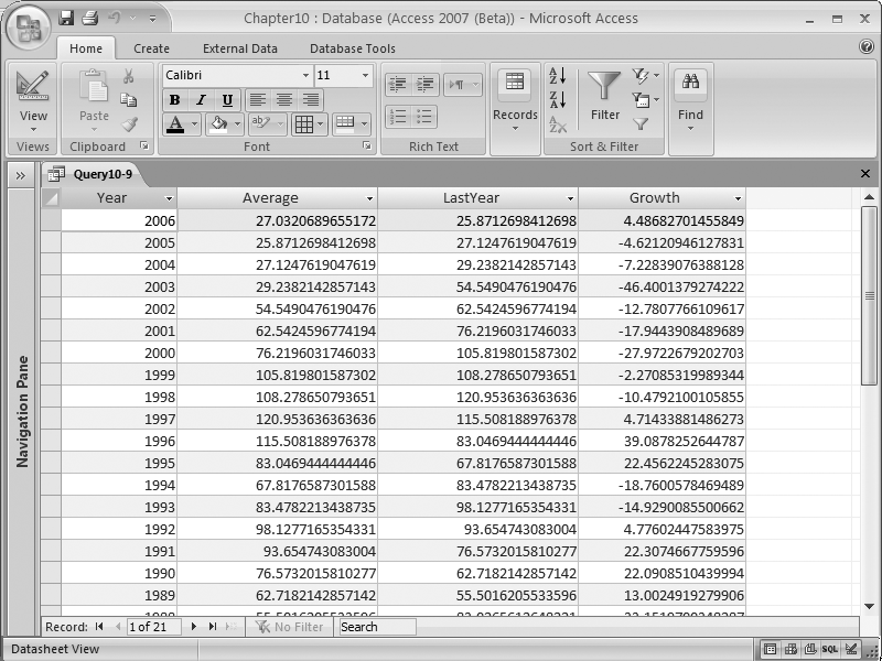
You can use a SELECT statement like this to compute annual growth rate:

	SELECT Year(Date) As Year, Avg(DisneyClose) As Average,
	   (Select Avg(DisneyClose) From Stocks b Where Year(b.date) = Year(a.Date) -1)
	      As LastYear,
	   (Average - LastYear) / LastYear * 100 As Growth
	FROM Stocks A
	Where DisneyClose Is Not Null
	Group By Year(Date)
	Order By Year(Date) Desc

The result is displayed in Figure 10-11.

Figure 10-11. Computing annual growth rate

The formula for calculating the growth rate looks like this:

	GrowthRate = (ThisYear – LastYear) / LastYear * 100

where ThisYear represents an average or sum of the values for the current year, and LastYear represents the same value computed for the previous year. GrowthRate represents the percentage increase or decrease over the previous year.

Note that you aren’t restricted to computing annual growth rates. As long as you’re consistent, you can use any time period (months, quarters, etc.). The key is that the growth rate is calculated by comparing values for the current time period with values for the previous time period and examining the percentage difference.

In addition, you don’t have to use averages to compute your statistics. In this case, they’re appropriate, as we’re looking at the average value of a stock price. However, if you’re looking at a different value, such as sales, it may be appropriate to compare the total sales rather than average sales figures.

A shortcoming of the SELECT statement used to generate the result in Figure 10-11 is that it computes the LastYear value by physically retrieving the rows for the previous year and calculating the average. This slows down the process considerably. You can compute the growth factor faster if you pre-calculate the average values for each year and store them in another table so you can access those values directly.

The following routine does exactly that. It opens two tables: one for input and the other for output. The input table uses a SELECT statement to get the averages by year, and orders the results in increasing order by year:

	Sub Example10_9()

	Dim InTable As ADODB.Recordset
	Dim OutTable As ADODB.Recordset
	Dim LagAverage As Double

	Set InTable = New ADODB.Recordset
	InTable.ActiveConnection = CurrentProject.Connection

	InTable.Open "SELECT Year(Date) As ThisYear, Avg(DisneyClose) As Average " & _
	     "From Stocks Where DisneyClose Is Not Null " & _
	     "Group By Year(Date) Order By Year(Date)", , adOpenForwardOnly, adLockReadOnly

	Set OutTable = New ADODB.Recordset
	OutTable.ActiveConnection = CurrentProject.Connection

	OutTable.Open "Growth", , adOpenDynamic, adLockOptimistic

	LagAverage = InTable.Fields("Average")
	OutTable.AddNew
	OutTable.Fields("Year") = InTable.Fields("ThisYear")
	OutTable.Fields("Growth") = Null
	OutTable.Update

	InTable.MoveNext

	Do While Not InTable.EOF
	   OutTable.AddNew
	   OutTable.Fields("Year") = InTable.Fields("ThisYear")
	   OutTable.Fields("Growth") = (InTable.Fields("Average") - LagAverage) _
	       / LagAverage * 100#
	   OutTable.Update

	   LagAverage = InTable.Fields("Average")
	   InTable.MoveNext

	Loop

	InTable.Close
	OutTable.Close

	End Sub

The average value for the first year is written to the output table. Growth is set to Null, as there isn’t a previous year’s data to use to perform the growth calculation. The average value for this year is saved into LagAverage.

Then, for each of the rest of the input rows, the corresponding output row is constructed by copying in the current year’s average value and computing the growth factor, using the average for this year and the previous year (stored in LagAverage). After the output row is saved, the current year’s average is saved into LagAverage before moving to the next row.

I’d like to compute a probability for each item in a table.

You can use a SELECT statement like this to determine the probability of each data item:

	SELECTRound(DisneyClose,0) AS StockValue, Count(*) AS Days,
	   (Select Count(*) From Stocks Where Date Between #1-1-2000# And #12-31-2005#)
	   AS Total, Days/Total AS Probability
	FROM Stocks
	WHERE Date Between #1/1/2000# And #12/31/2005#
	GROUP BY Round(DisneyClose,0)
	ORDER BY Round(DisneyClose,0);

The result of this query is displayed in Figure 10-12.

In this statement, each data item is rounded to the nearest dollar using the Round function. You can instead round to one or more decimal places by changing the 0 in the function to the number of decimal places you want to keep.

While the nested Select statement may seem expensive, it really isn’t. Jet only computes the value once because it doesn’t depend on anything from the current row. It can then return the value for each row it returns.

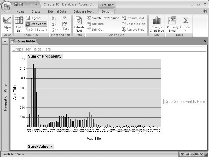
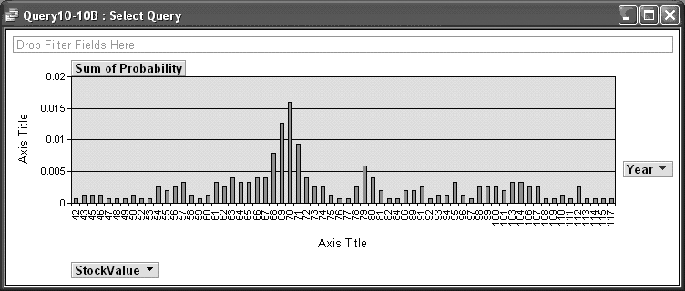
Figure 10-13 shows the probability distribution curve for the probability mass function. This was created by viewing the query results as a PivotChart, using StockValue as a category field and Sum of Probability as a series field, and dropping Probability onto the chart.

Figure 10-12. Computing the probability mass function for a set of data

While this doesn’t fit the traditional normal distribution, often called the “bell curve,” you can see that most of the stock prices fall within a narrow range of values. However, since the data spans five years, and the stock price varies over time, you may want to break it out by year.

If you rewrite the query to include a new column, Year(Date), and include this field in the GROUP BY clause, you can construct a new PivotChart in which you can select data from one or more years:

	SELECT Round(DisneyClose,0) AS StockValue, Year(Date) As Year, Count(*) AS Days,
	   (Select Count(*) From Stocks Where Date Between #1-1-2000# And #12-31-2005#) AS
	      Total,
	   Days/Total ASProbability
	FROM Stocks
	WHERE Date Between #1/1/2000# And #12/31/2005#
	GROUP BY Round(DisneyClose,0), Year(Date)
	ORDER BY Round(DisneyClose,0), Year(Date)

You can then easily compare the distribution of the data for different years. The distribution for 2000, for example (shown in Figure 10-14), is significantly different from the distribution for 2005 (shown in Figure 10-15).

Figure 10-13. The probability distribution curve for the probability mass function

Figure 10-14. In 2000, stock prices ranged between $42 and $117, with a price of $70 occurring most often

Figure 10-15. In 2005, stock prices ranged between $24 and $28, with a price of $25 occurring most often

I’d like to learn more about my data’s distribution by computing the kurtosis.

You can use the following routine to compute the kurtosis (i.e., the “peakedness” of the distribution of values) of a data set:

	Sub Example10_11()

	Dim rs As ADODB.Recordset
	Dim DisneyAvg As Double
	Dim DisneyVal As Double
	Dim Sum2 As Double
	Dim Sum4 As Double
	Dim TotalRows As Double
	Dim temp As Double
	DimKurtosis As Double

	Dim StdError As Double
	Set rs = New ADODB.Recordset
	rs.ActiveConnection = CurrentProject.Connection

	rs.Open "SELECT Avg(DisneyClose) AS AvgDisney, " & _
	   "Count(*) As TotalRows FROM Stocks " & _
	   "WHERE Date Between #1/1/2000# And #12/31/2005#", , _
	   adOpenForwardOnly, adLockReadOnly

	DisneyAvg = rs.Fields("AvgDisney")
	TotalRows = rs.Fields("TotalRows")

	rs.Close

	rs.Open "Select DisneyClose From Stocks " & _
	   "Where Date Between #1-1-2000# And #12-31-2005#", , _
	   adOpenStatic, adLockReadOnly

	Sum2 = 0
	Sum4 = 0

	Do While Not rs.EOF
	   DisneyVal = rs.Fields("DisneyClose")

	   temp = (DisneyVal - DisneyAvg) * (DisneyVal - DisneyAvg)

	   Sum2 = Sum2 + temp
	   Sum4 = Sum4 + temp * temp

	   rs.MoveNext

	Loop

	rs.Close

	Kurtosis = (TotalRows * Sum4 / (Sum2 * Sum2)) - 3
	StdError = Sqr(24 / TotalRows)

	Debug.Print "Kurtosis = ", Kurtosis
	Debug.Print "Standard error = ", StdError

	If Kurtosis > 2 * StdError Then
	   Debug.Print "Peaked distribution"

	ElseIf Kurtosis < -2 * StdError Then
	   Debug.Print "Flat distribution"

	Else
	   Debug.Print "Normal distribution"

	End If

	End Sub

The routine begins by executing a SELECT statement to return the number of rows in the sample along with the average value for the specified column. It then retrieves each of the individual values from the table, and sums the differences between the values and the average squared, and the differences between the values and the average raised to the fourth power.

Once all of the rows in the table have been processed, kurtosis can be computed by multiplying the number of rows times the sum of the difference between the current value and the average value raised to the fourth power. This value is then divided by the square of the sum of the differences between the current value and the average value squared. Finally, subtracting from the previous result completes the calculation for kurtosis.

Here is the formula to compute kurtosis:

	           N * Σ (x − X)4
	Kurtosis = --------------- - 3
	           ( Σ (x − X)2 )2

N is the number of values, x is the current value, and X is the average value.

A perfect normal distribution will return a kurtosis of 0. A negative value indicates the distribution is relatively flat, while a positive value means the distribution is relatively peaked.

Looking at the kurtosis can reveal what has caused the variance in a distribution. A higher value for kurtosis indicates the variance was caused by infrequent extreme deviations, while a lower value indicates it was caused by more frequent, modestly sized deviations.

To determine if the kurtosis value is significantly different from zero, you can use the following formula to compute the standard error:

	sqrt(24/number of items)

One advantage of computing kurtosis is that you can use the result to determine whether the data is outside the range of a normal distribution. If so, you won’t be able to trust the results from any statistical tests that assume a normal distribution.

How can I determine if my data has asymmetric “tails” when compared to the tails associated with a normal distribution?

The following code computes the skew (i.e., the asymmetry of the distribution of values) for a given column of data:

	Sub Example10_12()

	Dim rs As ADODB.Recordset
	Dim DisneyAvg As Double
	Dim DisneyVal As Double
	Dim Sum2 As Double
	Dim Sum3 As Double
	Dim TotalRows As Double
	Dim Skewness As Double
	Dim StdError As Double

	Set rs = New ADODB.Recordset
	rs.ActiveConnection = CurrentProject.Connection

	rs.Open "SELECT Avg(DisneyClose) AS AvgDisney, " & _
	   "Count(*) As TotalRows FROM Stocks " & _
	   "WHERE Date Between #1/1/2000# And #12/31/2005#", , _
	   adOpenForwardOnly, adLockReadOnly

	DisneyAvg = rs.Fields("AvgDisney")
	TotalRows = rs.Fields("TotalRows")

	rs.Close

	rs.Open "Select DisneyClose From Stocks " & _
	   "Where Date Between #1-1-2000# And #12-31-2005#", , _
	   adOpenStatic, adLockReadOnly

	Sum2 = 0
	Sum3 = 0

	Do While Not rs.EOF
	   DisneyVal = rs.Fields("DisneyClose")

	   Sum2 = Sum2 + (DisneyVal - DisneyAvg) * (DisneyVal - DisneyAvg)
	   Sum3 = Sum3 + (DisneyVal - DisneyAvg) * (DisneyVal - DisneyAvg) * _
	       (DisneyVal - DisneyAvg)
	   rs.MoveNext

	Loop

	rs.CloseSkewness = Sqr(TotalRows) * Sum3 / (Sum2 ^ 1.5)
	StdError = Sqr(6 / TotalRows)

	Debug.Print "Skewness = ", Skewness
	Debug.Print "Standard error = ", StdError

	If Skewness > 2 * StdError Then
	   Debug.Print "Skewed to the right"

	ElseIf Skewness < -2 * StdError Then
	   Debug.Print "Skewed to the left"

	Else
	   Debug.Print "Normal distribution"

	End If

	End Sub

The code used to compute skew is similar to the one used to compute kurtosis (see Computing the Kurtosis to Understand the Peakedness or Flatness of a Probability Mass Distribution).

The total number of values and the average value are computed for the entire set of data. Then, each row of data is processed, and the square and the cube of the difference between each item’s value—and the average for all values—are summed over the selected rows. Finally, the square root of the number of rows is multiplied by the sum of cubes, and then the total is divided by the sum of squares raised to the 1.5 power.

Here is the formula to compute skew:

	       N1/2 * Σ (x – X)3
	Skew = ----------------
	       ( Σ (x – X)2 )3/2

where N is the number of values, x is the current value, and X is the average value.

In a perfect normal distribution, both tails of the distribution will mirror each other, and the skew will have a value of 0. However, in real life, the tails are likely to be asymmetric. Testing for skewness determines whether the distribution is skewed to one side. A positive value means the distribution is skewed to the right, while a negative value means the data is skewed to the left.

Because most data can have a random component, however, you may compute a nonzero value for skew and still have a normal distribution. The standard error for skew can be computed with the following formula:

	sqrt(6/number of items)

Generally, skew values that are greater than twice the standard error are considered outside the range of a normal distribution.

I want to extract a range of data from my database by percentile.

Suppose you want to choose the top 10 percent of values in a particular column. You can do this with a SELECT statement that retrieves all possible values for the column, sorts them in descending order so that the highest values are listed first, and then returns the top 10 percent of the values:

	SELECT Top 10 Percent DisneyClose
	FROM StocksORDER BY DisneyClose Desc

If you want the bottom 10 percent, simply change the ORDER BY clause to sort the data in ascending order, like this:

	SELECT Top 10 Percent DisneyClose
	FROM Stocks
	ORDER BY DisneyClose Asc

What if you want to choose a range of values from the middle? You might be tempted to use a SELECT statement like this:

	SELECT Top 10 Percent DisneyClose
	FROM Stocks
	WHERE Not DisneyClose In
	   (Select Top 10 Percent DisneyClose
	   From Stocks
	   Order By DisneyClose Desc)
	ORDER BY DisneyClose Desc

This statement retrieves the top 10 percent of the rows from the table, but only if they’re not already in the top 10 percent. In other words, it effectively returns the second 10 percent.

The big problem with this approach is that the query is very inefficient because it runs the nested Select statement each time it processes a new row. A better approach would be to select the top 20 percent of the rows, place them into a separate table, and then select the bottom half of the new table. This would give you the same result, but with a lot less processing (although it does require you to run two queries and use a temporary table to get your result).

If you frequently select rows this way, you’d be better off using the following routine to pre-calculate the percentile value for each row and storing the results in a separate table:

	Sub Example10_13()

	Dim intable As ADODB.Recordset
	Dim outtable As ADODB.Recordset
	Dim Count As Long

	Set intable = New ADODB.Recordset
	intable.ActiveConnection = CurrentProject.Connection

	intable.Open "SELECT Date, DisneyClose As [Value], " & _
	    "(Select Count(*) From Stocks " & _
	    " Where DisneyClose Is Not Null) As Total " & _
	    "From Stocks " & _
	    "Where DisneyClose Is Not Null " & _
	    "Order By DisneyClose", , adOpenStatic, adLockReadOnly

	Set outtable = New ADODB.Recordset
	outtable.ActiveConnection = CurrentProject.Connection
	outtable.Open "Percentage", , adOpenDynamic, adLockOptimistic

	Count = 0

	Do While Not intable.EOF
	   outtable.AddNew
	   outtable.Fields("Date") = intable.Fields("Date")
	   outtable.Fields("Value") = intable.Fields("Value")
	   outtable.Fields("Percentage") = Count / intable.Fields("Total") * 100#
	   outtable.Update
	   intable.MoveNext

	   Count = Count + 1

	Loop

	intable.Close
	outtable.Close

	End Sub

This routine begins by selecting all of the data you may wish to use and sorting it in the proper order. It also computes the total number of rows that will be returned to avoid querying the database twice. Next, it opens a second Recordset that will hold the processed data.

The routine then loops through each row of the input table and copies the Date and Value fields to the output table. It also computes the row’s relative percentile, and stores that value in the output table. Finally, it closes both tables before returning.

Once this work table has been generated, you can construct statements to retrieve data between any two percentiles. For example, this Select statement retrieves all rows between the 80th and 90th percentiles:

	Select Date, Value
	From Percentage
	Where Percentage Is Between 80 and 90

I’d like to know the rank of a particular data value in my database.

One way to compute the rank of a particular data value is to create an append query like this one:

	INSERT INTO Rank
	SELECT Date AS [Date], DisneyClose AS [Value]
	FROM Stocks
	WHERE DisneyClose Is Not Null
	ORDER BY DisneyClose DESC;

You’ll also need to create an empty table with matching fields and an AutoNumber field. When you run the query, the AutoNumber field will automatically assign a sequential number to each new row. Because the rows are stored in the table from highest to lowest, the highest value will have a rank of 1, while the lowest will have a rank equal to the number of rows in the table.

Using this approach to automatically generate ranks has the advantage of requiring no programming. However, each time you run the append query, you’ll need to delete and re-create the output table to ensure that the AutoNumber field starts numbering from 1. Alternatively, you could create a generic Rank table and create a new copy of the table each time you want to run the query.

However, a better approach would be to modify the routine used in Returning a Range of Data by Percentile to regenerate the data each time, thus avoiding the problems with the AutoNumber field.

Here’s the updated routine:

	Sub Example10_14()

	Dim intable As ADODB.Recordset
	Dim outtable As ADODB.Recordset
	Dim Count As Long

	Set intable = New ADODB.Recordset
	intable.ActiveConnection = CurrentProject.Connection

	intable.Open "SELECT Date, DisneyClose As [Value] " & _
	    "From Stocks " & _
	    "Where DisneyClose Is Not Null " & _
	    "Order By DisneyClose Desc", , adOpenStatic, adLockReadOnly

	Set outtable = New ADODB.Recordset
	outtable.ActiveConnection = CurrentProject.Connection
	outtable.Open "[Table10-14]", , adOpenDynamic, adLockOptimistic

	Count = 1

	Do While Not intable.EOF
	   outtable.AddNew
	   outtable.Fields("Date") = intable.Fields("Date")
	   outtable.Fields("Value") = intable.Fields("Value")
	   outtable.Fields("Rank") = Count
	   outtable.Update
	   intable.MoveNext

	   Count = Count + 1

	Loop

	intable.Close
	outtable.Close

	End Sub

The routine begins by creating an input Recordset containing the desired data items in the proper order. Next, it opens the output Recordset. After that, each row is copied from the input Recordset to the output Recordset, and a sequential counter is assigned to each new row’s Rank field. Finally, the routine finishes the process by closing the input and output Recordsets.

I’d like to use linear regression to determine the slope and intercept point for two columns of data.

The following routine computes the slope and y intercept point for two sets of values. It’s based on the code originally used in Computing the Kurtosis to Understand the Peakedness or Flatness of a Probability Mass Distribution:

	Sub Example10_15()

	Dim rs As ADODB.Recordset
	Dim DisneyAvg As Double
	Dim TimeWarnerAvg As Double
	Dim DisneyVal As Double
	Dim TimeWarnerVal As Double
	Dim Sum1 As Double
	Dim Sum2 As Double
	Dim TotalRows As Double
	Dim Slope As Double
	Dim YIntercept As Double

	Set rs = New ADODB.Recordset
	rs.ActiveConnection = CurrentProject.Connection

	rs.Open "SELECT Avg(DisneyClose) AS AvgDisney, " & _
	   "Avg(TimeWarnerClose) As AvgTimeWarner " & _
	   "FROM Stocks WHERE Date Between #1/1/2000# And #12/31/2005#", , _
	   adOpenForwardOnly, adLockReadOnly

	DisneyAvg = rs.Fields("AvgDisney")
	TimeWarnerAvg = rs.Fields("AvgTimeWarner")

	rs.Close

	rs.Open "Select DisneyClose, TimeWarnerClose " & _
	   "From Stocks Where Date Between #1-1-2000# And #12-31-2005#", , _
	   adOpenStatic, adLockReadOnly

	Sum1 = 0
	Sum2 = 0

	Do While Not rs.EOF
	   DisneyVal = rs.Fields("DisneyClose")
	   TimeWarnerVal = rs.Fields("TimeWarnerClose")

	   Sum1 = Sum1 + (DisneyVal - DisneyAvg) * (TimeWarnerVal - TimeWarnerAvg)
	   Sum2 = Sum2 + (DisneyVal - DisneyAvg) * (DisneyVal - DisneyAvg)

	   rs.MoveNext

	Loop

	rs.Close
	
	Slope = Sum1 / Sum2
	YIntercept = TimeWarnerAvg - Slope * DisneyAvg

	Debug.Print "Slope= ", Slope
	Debug.Print "Y intercept= ", YIntercept
	
	End Sub

The routine begins by getting the average values for the two different columns. It then opens a Recordset that retrieves each individual pair of values. Next, it processes the data. Two sums are kept. The first sum is computed by subtracting each value from its column average and then multiplying the two resulting values together. The second sum is the square of the difference between the first value and its column average.

Once all the data has been processed, the routine computes the slope by dividing the first sum by the second. The y intercept point is then computed by plugging the average values for each column into the basic equation for a line using the newly computed value for slope.

Linear regression attempts to find the best possible straight line that matches a given set of pairs of data. The line is represented by slope and y intercept, where:

	        Σ ( x – X ) ( y – Y )
	Slope = ----------------------
	        Σ ( x – X )2

and:

	y intercept = Y – Slope X

x and y are individual data points, and X and Y represent the averages for of all of the x and y values, respectively.

I’d like to measure the volatility of my data to know how much values move around.

Volatility is a measure of uncertainty (risk) in the price movement of a stock, option, or other financial instrument. An alternate definition is that volatility is the dispersion of individual values around the mean of a set of data.

There are various approaches to calculating volatility, and, in a nutshell, there are two basic types of volatility: historical and implied. Historical volatility is easier to measure because the calculation is based on known values. Implied volatility is trickier because the purpose here is to guesstimate the level of volatility that will occur in the future (be that tomorrow, next month, or next year). In other words, implied volatility is calculated for forecasting purposes.

One reasonable approach to calculating volatility is to simply use the standard deviation as the measure. A standard deviation measurement requires >1 data points to provide a value. Figure 10-16 shows a table of values on the left, and the result of running a query against this data using the StDev aggregate function.

Figure 10-16. Calculating the standard deviation of a set of numbers

The volatility (as interpreted in this approach) is 2.7226562446208. But what does this tell us about the data? As a rule:

A standard deviation of 2.722656 is relatively small; therefore, the risk is also small. Standard deviation values can run from 0 to very large numbers—in the thousands or more. The standard deviation is a representation of the variance of the datum around the mean.

The SQL of the query in Figure 10-16 is:

	SELECT StDev(Table1.num) AS StDevOfnum FROM Table1

As you can see, it’s quite simple. A snapshot like the one this query provides can be useful, but in numerical analysis, trends are worth their weight in gold (or at least in silver). A series of volatility values may enable better analysis of the data. To determine the trend, a moving volatility line (similar to a moving average) is needed. Decision one is how many data points to base each standard deviation on. In the following example, we’ll use 20-day intervals.

Figure 10-17 shows a table listing a year’s worth of closing prices for Ford Motor Company stock (not all data is visible in the figure). The third column contains computations of volatility based on the given range (that is, from the closing price 20 days ago through the current date’s closing price).

Figure 10-17. Ford dates, prices, and volatility

As shown in Figure 10-18, we can use this data to plot a moving volatility line along with the prices. The figure contains two charts, one on top of the other. The bottom chart is a plot of the second column from Figure 10-17, and the top chart is a plot of the third column.

In Figure 10-17, you’ll notice that the first 14 rows show the same value in the third column. This is because a change in the volatility calculation’s result will not appear until 20 days into the data. The 14 rows actually comprise 20 calendar days because the column of dates does not include weekends or holidays (when the markets are closed). Considering this factor alone, it is obvious that there are numerous ways to calculate the volatility. For example, a similar but more developed process might include only trading days in the 20-day ranges.

Figure 10-18. Ford closing prices charted along with volatility

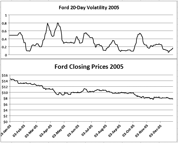
Because the values for the first 20 days do not vary (as there is no preceding data), the first bit of the volatility line in Figure 10-17 is flat. Only after 20 days does the line vary.

Here is the VBA code routine that produced the results in the third column in Figure 10-1:

	Sub fill_volatility()
	Dim conn As ADODB.Connection
	Set conn = CurrentProject.Connection
	Dim rs As New ADODB.Recordset
	rs.Open "Select * From Ford", conn, adOpenDynamic, adLockOptimistic
	Dim rs2 As New ADODB.Recordset
	Dim arr(20)
	Dim arr_count As Integer
	
	Do Until rs.EOF
	   ssql = "Select Clos from Ford Where" & _
	       "(Dte Between #" & rs.Fields("Dte") - 20 & _
	       "# And #" & rs.Fields("Dte") & "#) Order By Dte "
	   rs2.Open ssql, conn, adOpenKeyset, adLockOptimistic
	   arr_count = 0
	   Do Until rs2.EOF
	      arr(arr_count) = rs2.Fields("Clos")
	      arr_count = arr_count + 1
	      rs2.MoveNext
	   Loop
	
	   rs.Fields("Volatility") = Excel.WorksheetFunction.StDev(arr())
	   rs2.Close

	rs.MoveNext
	Loop
	rs.Close
	Set rs = Nothing
	Set conn = Nothing
	MsgBox "done"
	End Sub

The standard deviation is returned using Excel’s version of the StDev function. A reference to the Excel library is therefore required to run this routine. You can set the reference in the VB Editor, under Tools → References.

Those who attempt to make profits on fast price changes, such as day or swing traders, view high volatility as a positive thing. Conversely, investors who are in for the long haul tend to prefer securities with low volatility. Volatility has a positive correlation with risk, which means an investment with high volatility is, well, risky—not something that’s typically seen as desirable in long-term investments.

There are many formulas for calculating risk, and people tend to select methods that suit their particular circumstances (often having to do with the type of investment vehicle—stock, option, etc.). Unlike other formulas, volatility is broadly used to deter-mine the variance among a set of values. However, as you’ve seen, many different approaches can be taken to determine the volatility.

A major consideration is whether you’re attempting to calculate historical volatility (which provides answers based on existing data and is useful for backtesting, or seeing whether a given investing approach would have been successful) or implied volatility (which provides a guess as to the level of volatility in the future). Clearly, the latter is more involved because “assumptions” must be included within the calculations. This leads to complex formulas. Perhaps the best-known implied volatility method is the Black-Scholes model. This model is a standard for determining the future volatility of options. Options have more data points to consider than vanilla stock investments; calculations must involve the price of the option, the length of the option until expiration, and the expected value at the end of the option’s life.