9
Deep Reinforcement Learning
Reinforcement Learning (RL) is a framework that is used by an agent for decision making. The agent is not necessarily a software entity, such as you might see in video games. Instead, it could be embodied in hardware such as a robot or an autonomous car. An embodied agent is probably the best way to fully appreciate and utilize RL, since a physical entity interacts with the real world and receives responses.
The agent is situated within an environment. The environment has a state that can be partially or fully observable. The agent has a set of actions that it can use to interact with its environment. The result of an action transitions the environment to a new state. A corresponding scalar reward is received after executing an action.
The goal of the agent is to maximize the accumulated future reward by learning a policy that will decide which action to take given a state.
RL has a strong similarity to human psychology. Humans learn by experiencing the world. Wrong actions result in a certain form of penalty and should be avoided in the future, whilst actions that are correct are rewarded and should be encouraged. This strong similarity to human psychology has convinced many researchers to believe that RL can lead us toward true Artificial Intelligence (AI).
RL has been around for decades. However, beyond simple world models, RL has struggled to scale. This is where Deep Learning (DL) came into play. It solved this scalability problem, which opened up the era of Deep Reinforcement Learning (DRL). In this chapter, our focus is on DRL. One of the notable examples in DRL is the work of DeepMind on agents that were able to surpass the best human performance on different video games.
In this chapter, we discuss both RL and DRL.
In summary, the goal of this chapter is to present:
- The principles of RL
- The RL technique, Q-learning
- Advanced topics, including Deep Q-Network (DQN), and Double Q-Learning (DDQN)
- Instructions on how to implement RL on Python and DRL using
tf.keras
Let's start with the fundamentals, the principles behind RL.
1. Principles of Reinforcement Learning (RL)
Figure 9.1.1 shows the perception-action-learning loop that is used to describe RL. The environment is a soda can sitting on the floor. The agent is a mobile robot whose goal is to pick up the soda can. It observes the environment around it and tracks the location of the soda can through an onboard camera. The observation is summarized in a form of a state that the robot will use to decide which action to take. The actions it takes may pertain to low-level control, such as the rotation angle/speed of each wheel, the rotation angle/speed of each joint of the arm, and whether the gripper is open or closed.
Alternatively, the actions may be high-level control moves such as moving the robot forward/backward, steering with a certain angle, and grab/release. Any action that moves the gripper away from the soda receives a negative reward. Any action that closes the gap between the gripper location and the soda receives a positive reward. When the robot arm successfully picks up the soda can, it receives a big positive reward. The goal of RL is to learn the optimal policy that helps the robot to decide which action to take given a state to maximize the accumulated discounted reward:

Figure 9.1.1: The perception-action-learning loop in RL
Formally, the RL problem can be described as a Markov decision process (MDP).
For simplicity, we'll assume a deterministic environment where a certain action in a given state will consistently result in a known next state and reward. In a later section of this chapter, we'll look at how to consider stochasticity. At timestep t:
- The environment is in a state, st, from the state space,
 , which may be discrete or continuous. The starting state is s0, while the terminal state is sT.
 - The agent takes an action, sa,from the action space,
 , by obeying the policy,
  .
.  may be discrete or continuous.
 - The environment transitions to a new state, st+1, using the state transition dynamics
 . The next state is only dependent on the current state and action.
  is not known to the agent.
 - The agent receives a scalar reward using a reward function, rt+1 = R(st, at), with
 . The reward is only dependent on the current state and action.
  is not known to the agent.
 - Future rewards are discounted by
 , where
  and k is the future timestep.
 - Horizon, H, is the number of timesteps, T, needed to complete one episode from s0 to sT.
The environment may be fully or partially observable. The latter is also known as a partially observable MDP or POMDP. Most of the time, it's unrealistic to fully observe the environment. To improve the observability, past observations are also taken into consideration with the current observation. The state comprises the sufficient observations about the environment for the policy to decide on which action to take. Recalling Figure 9.1.1, this could be the three dimensional position of the soda can with respect to the robot gripper as estimated by the robot camera.
Every time the environment transitions to a new state, the agent receives a scalar reward, rt+1. In Figure 9.1.1, the reward could be +1 whenever the robot gets closer to the soda can, -1 whenever it gets farther away, and +100 when it closes the gripper and successfully picks up the soda can. The goal of the agent is to learn an optimal policy, ![]() , that maximizes the return from all states:
, that maximizes the return from all states:
 (Equation 9.1.1)
The return is defined as the discounted cumulative reward,  . It can be observed from Equation 9.1.1 that future rewards have lower weights compared to immediate rewards since generally,
 ![]() where
where ![]() . At the extremes, when
. At the extremes, when ![]() , only the immediate reward matters. When
, only the immediate reward matters. When ![]() , future rewards have the same weight as the immediate reward.
, future rewards have the same weight as the immediate reward.
Return can be interpreted as a measure of the value of a given state by following an arbitrary policy, ![]() :
:
 (Equation 9.1.2)
To put the RL problem in another way, the goal of the agent is to learn the optimal policy that maximizes ![]() for all states s:
for all states s:
 (Equation 9.1.3)
The value function of the optimal policy is simply ![]() . In Figure 9.1.1, the optimal policy is the one that generates the shortest sequence of actions that brings the robot closer and closer to the soda can until it is fetched. The closer the state to the goal state, the higher its value. The sequence of events leading to the goal (or terminal state) can be modeled as the trajectory or rollout of the policy:
. In Figure 9.1.1, the optimal policy is the one that generates the shortest sequence of actions that brings the robot closer and closer to the soda can until it is fetched. The closer the state to the goal state, the higher its value. The sequence of events leading to the goal (or terminal state) can be modeled as the trajectory or rollout of the policy:
 (Equation 9.1.4)
If the MDP is episodic, when the agent reaches the terminal state, sT, the state is reset to s0. If T is finite, we have a finite horizon. Otherwise, the horizon is infinite. In Figure 9.1.1, if the MDP is episodic, after collecting the soda can, the robot may look for another soda can to pick up and the RL problem repeats.
A key objective of RL is therefore to find a policy that maximizes the value of each state. In the next section, we will present a learning algorithm for the policy that can be used to maximize the value function.
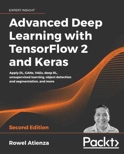
2. The Q value
If the RL problem is to find ![]() , how does the agent learn by interacting with the environment? Equation 9.1.3 does not explicitly indicate the action to try and the succeeding state to compute the return. In RL, it is easier to learn
, how does the agent learn by interacting with the environment? Equation 9.1.3 does not explicitly indicate the action to try and the succeeding state to compute the return. In RL, it is easier to learn ![]() by using the Q value:
by using the Q value:
 (Equation 9.2.1)
where:
 (Equation 9.2.2)
In other words, instead of finding the policy that maximizes the value for all states, Equation 9.2.1 looks for the action that maximizes the quality (Q) value for all states. After finding the Q value function, ![]() and hence
and hence ![]() are determined by Equation 9.2.2 and Equation 9.1.3, respectively.
are determined by Equation 9.2.2 and Equation 9.1.3, respectively.
If, for every action, the reward and the next state can be observed, we can formulate the following iterative or trial-and-error algorithm to learn the Q value:
 (Equation 9.2.3)
For notational simplicity, ![]() and
and ![]() are the next state and action, respectively. Equation 9.2.3 is known as the Bellman equation, which is the core of the Q-learning algorithm. Q-learning attempts to approximate the first-order expansion of return or value (Equation 9.1.2) as a function of both current state and action. From zero knowledge of the dynamics of the environment, the agent tries an action
are the next state and action, respectively. Equation 9.2.3 is known as the Bellman equation, which is the core of the Q-learning algorithm. Q-learning attempts to approximate the first-order expansion of return or value (Equation 9.1.2) as a function of both current state and action. From zero knowledge of the dynamics of the environment, the agent tries an action ![]() , observes what happens in the form of a reward,
, observes what happens in the form of a reward, ![]() , and next state,
, and next state, ![]() .
. ![]() chooses the next logical action that will give the maximum Q value for the next state. With all terms in Equation 9.2.3 known, the Q value for that current state-action pair is updated. Doing the update iteratively will eventually enable the agent to learn the Q value function.
chooses the next logical action that will give the maximum Q value for the next state. With all terms in Equation 9.2.3 known, the Q value for that current state-action pair is updated. Doing the update iteratively will eventually enable the agent to learn the Q value function.
Q-learning is an off-policy RL algorithm. It learns how to improve a policy by not directly sampling experiences from that policy. In other words, the Q values are learned independent of the underlying policy being used by the agent. When the Q value function has converged, only then is the optimal policy determined using Equation 9.2.1.
Before giving an example of how to use Q-learning, note that the agent must continually explore its environment while gradually taking advantage of what it has learned so far. This is one of the issues in RL – finding the right balance between exploration and exploitation. Generally, during the start of learning, the action is random (exploration). As the learning progresses, the agent takes advantage of the Q value (exploitation). For example, at the start, 90% of the action is random and 10% stems from the Q value function. At the end of each episode, this is gradually decreased. Eventually, the action is 10% random and 90% from the Q value function.
In the next section, we will give a concrete example as to how Q-learning is used in a simple deterministic environment.
3. Q-learning example
To illustrate the Q-learning algorithm, we need to consider a simple deterministic environment, as shown in Figure 9.3.1. The environment has six states.
The rewards for allowed transitions are shown. The reward is non-zero in two cases. Transition to the Goal (G) state has a +100 reward, while moving into the Hole (H) state has a -100 reward. These two states are terminal states and constitute the end of one episode from the Start state:

Figure 9.3.1: Rewards in a simple deterministic world
To formalize the identity of each state, we use a (row, column) identifier as shown in Figure 9.3.2. Since the agent has not learned anything yet about its environment, the Q-table also shown in Figure 9.3.2 has zero initial values. In this example, the discount factor ![]() . Recall that in the estimate of the current Q value, the discount factor determines the weight of future Q values as a function of the number of steps,
. Recall that in the estimate of the current Q value, the discount factor determines the weight of future Q values as a function of the number of steps, ![]() . In Equation 9.2.3, we only consider the immediate future Q value,
. In Equation 9.2.3, we only consider the immediate future Q value, ![]() .
.

Figure 9.3.2: States in the simple deterministic environment and the agent's initial Q-table
Initially, the agent assumes a policy that selects a random action 90% of the time and exploits the Q-table 10% of the time. Suppose the first action is randomly chosen and indicates a move to the right. Figure 9.3.3 illustrates the computation of the new Q value of state (0, 0) for a move to the right. The next state is (0, 1). The reward is 0, and the maximum of all the next state's Q values is zero. Therefore, the Q value of state (0, 0) for a move to the right remains 0.
To easily track the initial state and next state, we use different shades of gray on both the environment and the Q-table—lighter gray for the initial state, and darker gray for the next state.
In choosing the next action for the next state, the candidate actions are in the thicker border:

Figure 9.3.3: Assuming the action taken by the agent is a move to the right, an update to the Q value of state (0, 0) is shown
Let's suppose that the next randomly chosen action is a move in a downward direction. Figure 9.3.4 shows no change in the Q value of state (0, 1) for the move in a downward direction:

Figure 9.3.4: Assuming the action chosen by the agent is a move down, an update to the Q value of state (0, 1) is shown
In Figure 9.3.5, the agent's third random action is a move to the right;

Figure 9.3.5: Assuming the action chosen by the agent is a move to the right, an update to the Q value of state (1, 1) is shown
It encountered the H state and received a -100 reward. This time, the update is non-zero. The new Q value for the state (1, 1) is -100 for the move to the right. Note that since this is a terminal state, there are no next states. One episode has just finished, and the agent returns to the Start state.
Let's suppose the agent is still in exploration mode, as shown in Figure 9.3.6:

Figure 9.3.6: Assuming the actions chosen by the agent are two successive moves to the right, an update to the Q value of state (0, 1) is shown
The first step it took for the second episode was a move to the right. As expected, the update is 0. However, the second random action it chose is also a move to the right. The agent reached the G state and received a big +100 reward. The Q value for the state (0, 1) moving to the right becomes 100. The second episode is done, and the agent goes back to the Start state.
At the beginning of the third episode, the random action taken by the agent is a move to the right. The Q value of state (0, 0) is now updated with a non-zero value because the next state's possible actions have 100 as the maximum Q value. Figure 9.3.7 shows the computation involved. The Q value of the next state (0, 1) ripples back to the earlier state (0, 0). It is like giving credit to the earlier states that helped in finding the G state.

Figure 9.3.7: Assuming the action chosen by the agent is a move to the right, an update to the Q value of state (0, 0) is shown
The progress in the Q-table has been substantial. In fact, in the next episode, if, for some reason, the policy decided to exploit the Q-table instead of randomly exploring the environment, the first action is to move to the right according to the computation in Figure 9.3.8. In the first row of the Q-table, the action that results in the maximum Q value is a move to the right. For the next state (0, 1), the second row of the Q-table suggests that the next action is still to move to the right. The agent has successfully reached its goal. The policy guided the agent on the right set of actions to achieve its goal:

Figure 9.3.8: In this instance, the agent's policy decided to exploit the Q-table to determine the action at states (0, 0) and (0, 1). The Q-table suggests moving to the right for both states
If the Q-learning algorithm continues to run indefinitely, the Q-table will converge. The assumptions for convergence are that the RL problem must be a deterministic MDP with bounded rewards, and all states are visited infinitely often.
In the next section, we will simulate the environment using Python. We will also show the code implementation of the Q-learning algorithm.
Q-Learning in Python
The environment and the Q-learning discussed in the previous section can be implemented in Python. Since the policy is just a simple table, at this point in time, there is no need to use the tf.keras library. Listing 9.3.1 shows q-learning-9.3.1.py, the implementation of the simple deterministic world (environment, agent, action, and Q-table algorithms) using the QWorld class. For conciseness, the functions dealing with the user interface are not shown.
In this example, the environment dynamics is represented by self.transition_table. At every action, self.transition_table determines the next state. The reward for executing an action is stored in self.reward_table. The two tables are consulted every time an action is executed by the step() function. The Q-learning algorithm is implemented by the update_q_table() function. Every time the agent needs to decide which action to take, it calls the act() function. The action may be randomly drawn or decided by the policy using the Q-table. The percentage chance that the action chosen is random is stored in the self.epsilon variable, which is updated by the update_epsilon() function using a fixed epsilon_decay.
Before executing the code in Listing 9.3.1, we need to run:
sudo pip3 install termcolor
to install the termcolor package. This package helps in visualizing text outputs on the Terminal.
The complete code can be found on GitHub at https://github.com/PacktPublishing/Advanced-Deep-Learning-with-Keras.
Listing 9.3.1: q-learning-9.3.1.py
A simple deterministic MDP with six states:
from collections import deque
import numpy as np
import argparse
import os
import time
from termcolor import colored
class QWorld:
    def __init__(self):
        """Simulated deterministic world made of 6 states.
        Q-Learning by Bellman Equation.
        """
        # 4 actions
        # 0 - Left, 1 - Down, 2 - Right, 3 - Up
        self.col = 4
        # 6 states
        self.row = 6
        # setup the environment
        self.q_table = np.zeros([self.row, self.col])
        self.init_transition_table()
        self.init_reward_table()
        # discount factor
        self.gamma = 0.9
        # 90% exploration, 10% exploitation
        self.epsilon = 0.9
        # exploration decays by this factor every episode
        self.epsilon_decay = 0.9
        # in the long run, 10% exploration, 90% exploitation
        self.epsilon_min = 0.1
        # reset the environment
        self.reset()
        self.is_explore = True
    def reset(self):
        """start of episode"""
        self.state = 0
        return self.state
    def is_in_win_state(self):
        """agent wins when the goal is reached"""
        return self.state == 2
    def init_reward_table(self):
        """
        0 - Left, 1 - Down, 2 - Right, 3 - Up
        ----------------
        | 0 | 0 | 100  |
        ----------------
        | 0 | 0 | -100 |
        ----------------
        """
        self.reward_table = np.zeros([self.row, self.col])
        self.reward_table[1, 2] = 100.
        self.reward_table[4, 2] = -100.
    def init_transition_table(self):
        """
        0 - Left, 1 - Down, 2 - Right, 3 - Up
        -------------
        | 0 | 1 | 2 |
        -------------
        | 3 | 4 | 5 |
        -------------
        """
        self.transition_table = np.zeros([self.row, self.col],
                                         dtype=int)
        self.transition_table[0, 0] = 0
        self.transition_table[0, 1] = 3
        self.transition_table[0, 2] = 1
        self.transition_table[0, 3] = 0
        self.transition_table[1, 0] = 0
        self.transition_table[1, 1] = 4
        self.transition_table[1, 2] = 2
        self.transition_table[1, 3] = 1
        # terminal Goal state
        self.transition_table[2, 0] = 2
        self.transition_table[2, 1] = 2
        self.transition_table[2, 2] = 2
        self.transition_table[2, 3] = 2
        self.transition_table[3, 0] = 3
        self.transition_table[3, 1] = 3
        self.transition_table[3, 2] = 4
        self.transition_table[3, 3] = 0
        self.transition_table[4, 0] = 3
        self.transition_table[4, 1] = 4
        self.transition_table[4, 2] = 5
        self.transition_table[4, 3] = 1
        # terminal Hole state
        self.transition_table[5, 0] = 5
        self.transition_table[5, 1] = 5
        self.transition_table[5, 2] = 5
        self.transition_table[5, 3] = 5
    def step(self, action):
        """execute the action on the environment
        Argument:
            action (tensor): An action in Action space
        Returns:
            next_state (tensor): next env state
            reward (float): reward received by the agent
            done (Bool): whether the terminal state
                is reached
        """
        # determine the next_state given state and action
        next_state = self.transition_table[self.state, action]
        # done is True if next_state is Goal or Hole
        done = next_state == 2 or next_state == 5
        # reward given the state and action
        reward = self.reward_table[self.state, action]
        # the enviroment is now in new state
        self.state = next_state
        return next_state, reward, done
    def act(self):
        """determine the next action
            either fr Q Table(exploitation) or
            random(exploration)
        Return:
            action (tensor): action that the agent
                must execute
        """
        # 0 - Left, 1 - Down, 2 - Right, 3 - Up
        # action is from exploration
        if np.random.rand() <= self.epsilon:
            # explore - do random action
            self.is_explore = True
            return np.random.choice(4,1)[0]
        # or action is from exploitation
        # exploit - choose action with max Q-value
        self.is_explore = False
        action = np.argmax(self.q_table[self.state])
        return action
    def update_q_table(self, state, action, reward, next_state):
        """Q-Learning - update the Q Table using Q(s, a)
        Arguments:
            state (tensor) : agent state
            action (tensor): action executed by the agent
            reward (float): reward after executing action
                for a given state
            next_state (tensor): next state after executing
                action for a given state
        """
        # Q(s, a) = reward + gamma * max_a' Q(s', a')
        q_value = self.gamma * np.amax(self.q_table[next_state])
        q_value += reward
        self.q_table[state, action] = q_value
    def update_epsilon(self):
        """update Exploration-Exploitation mix"""
        if self.epsilon > self.epsilon_min:
            self.epsilon *= self.epsilon_decay
The perception-action-learning loop is illustrated in Listing 9.3.2. At every episode, the environment resets to the Start state. The action to execute is chosen and applied to the environment. The reward and next state are observed and used to update the Q-table. The episode is completed (done = True) upon reaching the Goal or Hole state.
For this example, the Q-learning runs for 100 episodes or 10 wins, whichever comes first. Due to the decrease in the value of the self.epsilon variable at every episode, the agent starts to favor exploitation of the Q-table to determine the action to perform given a state. To see the Q-learning simulation, we simply need to run the following command:
python3 q-learning-9.3.1.py
Listing 9.3.2: q-learning-9.3.1.py
The main Q-learning loop:
    # state, action, reward, next state iteration
    for episode in range(episode_count):
        state = q_world.reset()
        done = False
        print_episode(episode, delay=delay)
        while not done:
            action = q_world.act()
            next_state, reward, done = q_world.step(action)
            q_world.update_q_table(state, action, reward, next_state)
            print_status(q_world, done, step, delay=delay)
            state = next_state
            # if episode is done, perform housekeeping
            if done:
                if q_world.is_in_win_state():
                    wins += 1
                    scores.append(step)
                    if wins > maxwins:
                        print(scores)
                        exit(0)
                # Exploration-Exploitation is updated every episode
                q_world.update_epsilon()
                step = 1
            else:
                step += 1
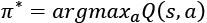
Figure 9.3.9 shows the screenshot if maxwins = 2000 (2000x Goal state is reached) and delay = 0. To see the final Q-table only, execute:
python3 q-learning-9.3.1.py --train
Figure 9.3.9: A screenshot showing the Q-table after 2,000 wins on the part of the agent
The Q-table has converged and shows the logical action that the agent can take given a state. For example, in the first row or state (0, 0), the policy advises a move to the right. The same goes for the state (0, 1) on the second row. The second action reaches the Goal state. The scores variable dump shows that the minimum number of steps taken decreases as the agent gets correct actions from the policy.
From Figure 9.3.9, we can compute the value of each state from Equation 9.2.2, ![]() . For example, for state (0, 0),
. For example, for state (0, 0), ![]() .
.
Figure 9.3.10 shows the value for each state.

Figure 9.3.10: The value for each state from Figure 9.3.9 and Equation 9.2.2
This simple example illustrated all elements of Q-learning for an agent in a simple deterministic world. In the next section, we will present the slight modification needed to take stochasticity into account.
4. Nondeterministic environment
In the event that the environment is nondeterministic, both the reward and action are probabilistic. The new system is a stochastic MDP. To reflect the nondeterministic reward, the new value function is:
 (Equation 9.4.1)
The Bellman equation is modified as:
 (Equation 9.4.2)
However, in this chapter, we will focus on deterministic environments. In the next section, we will present a more generalized Q-learning algorithm called Temporal-Difference (TD) learning.
5. Temporal-difference learning
Q-learning is a special case of a more generalized TD learning, ![]() . More specifically, it is a special case of one-step TD learning, TD(0):
. More specifically, it is a special case of one-step TD learning, TD(0):
 (Equation 9.5.1)
Where ![]() is the learning rate. Note that when
is the learning rate. Note that when ![]() , Equation 9.5.1 is similar to the Bellman equation. For simplicity, we also refer to Equation 9.5.1 as Q-learning, or generalized Q-learning.
, Equation 9.5.1 is similar to the Bellman equation. For simplicity, we also refer to Equation 9.5.1 as Q-learning, or generalized Q-learning.
Previously, we referred to Q-learning as an off-policy RL algorithm since it learns the Q value function without directly using the policy that it is trying to optimize. An example of an on-policy one-step TD-learning algorithm is SARSA, which is similar to Equation 9.5.1:
 (Equation 9.5.2)
The main difference is the use of the policy that is being optimized to determine ![]() . The terms
. The terms ![]() ,
, ![]() ,
, ![]() ,
, ![]() , and
, and ![]() (thus the name SARSA) must be known to update the Q value function every iteration. Both Q-learning and SARSA use existing estimates in the Q value iteration, a process known as bootstrapping. In bootstrapping, we update the current Q value estimate from the reward and the subsequent Q value estimate(s).
(thus the name SARSA) must be known to update the Q value function every iteration. Both Q-learning and SARSA use existing estimates in the Q value iteration, a process known as bootstrapping. In bootstrapping, we update the current Q value estimate from the reward and the subsequent Q value estimate(s).
Before presenting another example, there appears to be a need for a suitable RL simulation environment. Otherwise, we can only run RL simulations on very simple problems like in the previous example. Fortunately, OpenAI created Gym, https://gym.openai.com, which we'll cover in the following section.
Q-learning on OpenAI Gym
OpenAI Gym is a toolkit for developing and comparing RL algorithms. It works with most DL libraries, including tf.keras. The gym can be installed by running the following command:
sudo pip3 install gym
The gym has several environments where an RL algorithm can be tested against, such as toy text, classic control, algorithmic, Atari, and two-dimensional/three-dimensional robots. For example, FrozenLake-v0 (Figure 9.5.1) is a toy text environment similar to the simple deterministic world used in the Q-learning in Python example:

Figure 9.5.1: The FrozenLake-v0 environment in OpenAI Gym
FrozenLake-v0 has 12 states, the state marked S is the starting state, F is the frozen part of the lake, which is safe, H is the Hole state, which should be avoided, and G is the Goal state where the frisbee is located. The reward is +1 for transitioning to the Goal state. For all other states, the reward is zero.
In FrozenLake-v0, there are also four available actions (left, down, right, up) known as action space. However, unlike the simple deterministic world earlier, the actual movement direction is only partially dependent on the chosen action. There are two variations of the FrozenLake-v0 environment; slippery and non-slippery. As expected, the slippery mode is more challenging.
An action applied to FrozenLake-v0 returns the observation (equivalent to the next state), reward, done (whether the episode is finished), and a dictionary of debugging information. The observable attributes of the environment, known as observation space, are captured by the returned observation object.
Generalized Q-learning can be applied to the FrozenLake-v0 environment. Table 9.5.1 shows the improvement in performance of both slippery and non-slippery environments. A method of measuring the performance of the policy is the percentage of episodes executed that resulted in reaching the Goal state. The higher the percentage, the better. From the baseline of pure exploration (random action) of about 1.5%, the policy can achieve ~76% Goal state for the non-slippery environment and ~71% for the slippery environment. As expected, it is harder to control the slippery environment.
| Mode | Run | Approx % Goal |
|
Train non-slippery |
|
26 |
|
Test non-slippery |
|
76 |
|
Pure random action non-slippery |
|
1.5 |
|
Train slippery |
|
26 |
|
Test slippery |
|
71 |
|
Pure random slippery |
|
1.5 |
Table 9.5.1: Baseline and performance of generalized Q-learning on the FrozenLake-v0 environment with a learning rate = 0.5
The code can still be implemented in Python and NumPy since it only requires a Q-table. Listing 9.5.1 shows the implementation of the QAgent class. Apart from using the FrozenLake-v0 environment from OpenAI Gym, the most important change is the implementation of the generalized Q-learning, as defined by Equation 9.5.1 in the update_q_table() function.
Listing 9.5.1: q-frozenlake-9.5.1.py
Q-learning on the FrozenLake-v0 environment:
from collections import deque
import numpy as np
import argparse
import os
import time
import gym
from gym import wrappers, logger
class QAgent:
    def __init__(self,
                 observation_space,
                 action_space,
                 demo=False,
                 slippery=False,
                 episodes=40000):
        """Q-Learning agent on FrozenLake-v0 environment
        Arguments:
            observation_space (tensor): state space
            action_space (tensor): action space
            demo (Bool): whether for demo or training
            slippery (Bool): 2 versions of FLv0 env
            episodes (int): number of episodes to train
        """
        self.action_space = action_space
        # number of columns is equal to number of actions
        col = action_space.n
        # number of rows is equal to number of states
        row = observation_space.n
        # build Q Table with row x col dims
        self.q_table = np.zeros([row, col])
        # discount factor
        self.gamma = 0.9
        # initially 90% exploration, 10% exploitation
        self.epsilon = 0.9
        # iteratively applying decay til
        # 10% exploration/90% exploitation
        self.epsilon_min = 0.1
        self.epsilon_decay = self.epsilon_min / self.epsilon
        self.epsilon_decay = self.epsilon_decay **
                             (1. / float(episodes))
        # learning rate of Q-Learning
        self.learning_rate = 0.1
        # file where Q Table is saved on/restored fr
        if slippery:
            self.filename = 'q-frozenlake-slippery.npy'
        else:
            self.filename = 'q-frozenlake.npy'
        # demo or train mode
        self.demo = demo
        # if demo mode, no exploration
        if demo:
            self.epsilon = 0
    def act(self, state, is_explore=False):
        """determine the next action
            if random, choose from random action space
            else use the Q Table
        Arguments:
            state (tensor): agent's current state
            is_explore (Bool): exploration mode or not
        Return:
            action (tensor): action that the agent
                must execute
        """
        # 0 - left, 1 - Down, 2 - Right, 3 - Up
        if is_explore or np.random.rand() < self.epsilon:
            # explore - do random action
            return self.action_space.sample()
        # exploit - choose action with max Q-value
        action = np.argmax(self.q_table[state])
        return action
    def update_q_table(self, state, action, reward, next_state):
        """TD(0) learning (generalized Q-Learning) with learning rate
        Arguments:
            state (tensor): environment state
            action (tensor): action executed by the agent for
                the given state
            reward (float): reward received by the agent for
                executing the action
            next_state (tensor): the environment next state
        """
        # Q(s, a) +=
        # alpha * (reward + gamma * max_a' Q(s', a') - Q(s, a))
        q_value = self.gamma * np.amax(self.q_table[next_state])
        q_value += reward
        q_value -= self.q_table[state, action]
        q_value *= self.learning_rate
        q_value += self.q_table[state, action]
        self.q_table[state, action] = q_value
    def update_epsilon(self):
        """adjust epsilon"""
        if self.epsilon > self.epsilon_min:
            self.epsilon *= self.epsilon_decay
Listing 9.5.2 demonstrates the agent's perception-action-learning loop. At every episode, the environment resets by calling env.reset(). The action to execute is chosen by agent.act() and applied to the environment by env.step(action). The reward and next state are observed and used to update the Q-table.
After every action, the TD learning is executed by agent.update_q_table(). Due to the decrease in the value of the self.epsilon variable at every episode's call to agent.update_epsilon(), the agent starts to favor exploitation of Q-table to determine the action to perform given a state. The episode is completed (done = True) upon reaching the Goal or Hole state. For this example, the TD learning runs for 4,000 episodes.
Listing 9.5.2: q-frozenlake-9.5.1.py.
Q-learning loop for the FrozenLake-v0 environment:
    # loop for the specified number of episode
    for episode in range(episodes):
        state = env.reset()
        done = False
        while not done:
            # determine the agent's action given state
            action = agent.act(state, is_explore=args.explore)
            # get observable data
            next_state, reward, done, _ = env.step(action)
            # clear the screen before rendering the environment
            os.system('clear')
            # render the environment for human debugging
            env.render()
            # training of Q Table
            if done:
                # update exploration-exploitation ratio
                # reward > 0 only when Goal is reached
                # otherwise, it is a Hole
                if reward > 0:
                    wins += 1
            if not args.demo:
                agent.update_q_table(state,
                                     action,
                                     reward,
                                     next_state)
                agent.update_epsilon()
            state = next_state
            percent_wins = 100.0 * wins / (episode + 1)
The agent object can operate in either slippery or non-slippery mode. After training, the agent can exploit the Q-table to choose the action to execute given any policy, as shown in the test mode of Table 9.5.1. There is a huge performance boost in using the learned policy as demonstrated in Table 9.5.1. With the use of the gym, many lines of code in constructing the environment are no longer needed. For example, unlike in the previous example, with the use of OpenAI Gym, we do not need to create the state transition table and the rewards table.
This will help us to focus on building a working RL algorithm. To run the code in slow motion or have a delay of 1 second per action:
python3 q-frozenlake-9.5.1.py -d -t=1
In this section, we demonstrated Q-learning on a more challenging environment. We also introduced the OpenAI Gym. However, our environment is still a toy environment. What if we have a huge number of states or actions? In that case, it is no longer feasible to use a Q-table. In the next section, we will use a deep neural network to learn the Q-table.
6. Deep Q-Network (DQN)
Using the Q-table to implement Q-learning is fine in small discrete environments. However, when the environment has numerous states or is continuous, as in most cases, a Q-table is not feasible or practical. For example, if we are observing a state made of four continuous variables, the size of the table is infinite. Even if we attempt to discretize the four variables into 1,000 values each, the total number of rows in the table is a staggering 10004 = 1e12. Even after training, the table is sparse – most of the cells in this table are zero.
A solution to this problem is called DQN [2], which uses a deep neural network to approximate the Q-table, as shown in Figure 9.6.1. There are two approaches to building the Q-network:
- The input is the state-action pair, and the prediction is the Q value
- The input is the state, and the prediction is the Q value for each action
The first option is not optimal since the network will be called a number of times equal to the number of actions. The second is the preferred method. The Q-network is called only once.
The most desirable action is simply the action with the biggest Q value.

Figure 9.6.1: A deep Q-network
The data required to train the Q-network comes from the agent's experiences: ![]() . Each training sample is a unit of experience,
. Each training sample is a unit of experience, ![]() . At a given state at timestep
. At a given state at timestep ![]() ,
, ![]() , the action,
, the action, ![]() , is determined using the Q-learning algorithm similar to the previous section:
, is determined using the Q-learning algorithm similar to the previous section:
 (Equation 9.6.1)
For notational simplicity, we omit the subscript and the use of bold letters. Note that ![]() is the Q-network. Strictly speaking, it is
is the Q-network. Strictly speaking, it is ![]() since the action is moved to the prediction stage (in other words, output) as shown on the right of Figure 9.6.1. The action with the highest Q value is the action that is applied to the environment to get the reward,
since the action is moved to the prediction stage (in other words, output) as shown on the right of Figure 9.6.1. The action with the highest Q value is the action that is applied to the environment to get the reward, ![]() , the next state,
, the next state, ![]() , and a Boolean
, and a Boolean done, indicating whether the next state is terminal. From Equation 9.5.1 on generalized Q-learning, an MSE loss function can be determined by applying the chosen action:
 (Equation 9.6.2)
where all terms are familiar from the previous discussion on Q-learning and ![]() . The term
. The term ![]()
![]() . In other words, using the Q-network, predict the Q value of each action given the next state and get the maximum from among them. Note that at the terminal state,
. In other words, using the Q-network, predict the Q value of each action given the next state and get the maximum from among them. Note that at the terminal state, ![]() ,
, ![]() .
.
However, it turns out that training the Q-network is unstable. There are two problems causing the instability: 1) high correlation between samples; and 2) a non-stationary target. A high correlation is due to the sequential nature of sampling experiences. DQN addressed this issue by creating a buffer of experiences. The training data is randomly sampled from this buffer. This process is known as experience replay.
The issue of the non-stationary target is due to the target network ![]() that is modified after every mini batch of training. A small change in the target network can create a significant change in the policy, the data distribution, and the correlation between the current Q value and target Q value. This is resolved by freezing the weights of the target network for
that is modified after every mini batch of training. A small change in the target network can create a significant change in the policy, the data distribution, and the correlation between the current Q value and target Q value. This is resolved by freezing the weights of the target network for ![]() training steps. In other words, two identical Q-networks are created. The target Q-network parameters are copied from the Q-network under training every
training steps. In other words, two identical Q-networks are created. The target Q-network parameters are copied from the Q-network under training every ![]() training steps.
training steps.
The deep Q-network algorithm is summarized in Algorithm 9.6.1.
Algorithm 9.6.1: DQN algorithm
Require: Initialize replay memory ![]() to capacity
to capacity ![]()
Require: Initialize action-value function ![]() with random weights
with random weights ![]()
Require: Initialize target action-value function ![]() with weights
with weights ![]()
Require: Exploration rate, ![]() , and discount factor,
, and discount factor, ![]()
forepisode = 1, … , M,do:- Given initial state s
-
forstep = 1, … , T do: - Choose action

- Execute action
 , observe reward r, and Next state
- Store transition
 in
in 
- Update the state,

- // experience replay
- Sample a mini batch of episode experiences
 from
from 
-

- Perform gradient descent step on
 w.r.t. parameters
- // periodic update of target network
- Every
 steps,
  , in other words, set
-
end
end
Algorithm 9.6.1 sums up all the techniques needed in order to implement Q-learning on environments with discrete action space and continuous state space. In the next section, we will demonstrate how DQN is used in a more challenging OpenAI Gym environment.
DQN on Keras
To illustrate DQN, the CartPole-v0 environment of the OpenAI Gym is used. CartPole-v0 is a pole balancing problem. The goal is to keep the pole from falling over. The environment is two dimensional. The action space is made of two discrete actions (left and right movements). However, the state space is continuous and comprises four variables:
- Linear position
- Linear velocity
- Angle of rotation
- Angular velocity
The CartPole-v0 environment is shown in Figure 9.6.1:
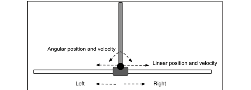
Figure 9.6.1: The CartPole-v0 environment
Initially, the pole is upright. A reward of +1 is provided for every timestep that the pole remains upright. The episode ends when the pole exceeds 15 degrees from the vertical, or 2.4 units from the center. The CartPole-v0 problem is considered solved if the average reward is 195.0 in 100 consecutive trials:
Listing 9.6.1 shows us the DQN implementation for CartPole-v0. The DQNAgent class represents the agent using DQN. Two Q-networks are created:
- A Q-network, or Q, in Algorithm 9.6.1
- A target Q-network, or Qtarget, in Algorithm 9.6.1
Both networks are MLP with 3 hidden layers of 256 units each. Both networks are created by means of the build_model() method. The Q-network is trained during experience replay, replay(). At a regular interval of C = 10 training steps, the Q-network parameters are copied to the target Q-network by update_weights(). This implements line 13, Qtarget = Q, in Algorithm 9.6.1. After every episode, the ratio of exploration-exploitation is decreased by update_epsilon() to take advantage of the learned policy.
Listing 9.6.1: dqn-cartpole-9.6.1.py
DQN in tf.keras:
class DQNAgent:
    def __init__(self,
                 state_space,
                 action_space,
                 episodes=500):
        """DQN Agent on CartPole-v0 environment
        Arguments:
            state_space (tensor): state space
            action_space (tensor): action space
            episodes (int): number of episodes to train
        """
        self.action_space = action_space
        # experience buffer
        self.memory = []
        # discount rate
        self.gamma = 0.9
        # initially 90% exploration, 10% exploitation
        self.epsilon = 1.0
        # iteratively applying decay til
        # 10% exploration/90% exploitation
        self.epsilon_min = 0.1
        self.epsilon_decay = self.epsilon_min / self.epsilon
        self.epsilon_decay = self.epsilon_decay **
                             (1. / float(episodes))
        # Q Network weights filename
        self.weights_file = 'dqn_cartpole.h5'
        # Q Network for training
        n_inputs = state_space.shape[0]
        n_outputs = action_space.n
        self.q_model = self.build_model(n_inputs, n_outputs)
        self.q_model.compile(loss='mse', optimizer=Adam())
        # target Q Network
        self.target_q_model = self.build_model(n_inputs, n_outputs)
        # copy Q Network params to target Q Network
        self.update_weights()
        self.replay_counter = 0
        self.ddqn = True if args.ddqn else False
    def build_model(self, n_inputs, n_outputs):
        """Q Network is 256-256-256 MLP
        Arguments:
            n_inputs (int): input dim
            n_outputs (int): output dim
        Return:
            q_model (Model): DQN
        """
        inputs = Input(shape=(n_inputs, ), name='state')
        x = Dense(256, activation='relu')(inputs)
        x = Dense(256, activation='relu')(x)
        x = Dense(256, activation='relu')(x)
        x = Dense(n_outputs,
                  activation='linear',
                  name='action')(x)
        q_model = Model(inputs, x)
        q_model.summary()
        return q_model
    def act(self, state):
        """eps-greedy policy
        Return:
            action (tensor): action to execute
        """
        if np.random.rand() < self.epsilon:
            # explore - do random action
            return self.action_space.sample()
        # exploit
        q_values = self.q_model.predict(state)
        # select the action with max Q-value
        action = np.argmax(q_values[0])
        return action
    def remember(self, state, action, reward, next_state, done):
        """store experiences in the replay buffer
        Arguments:
            state (tensor): env state
            action (tensor): agent action
            reward (float): reward received after executing
                action on state
            next_state (tensor): next state
        """
        item = (state, action, reward, next_state, done)
        self.memory.append(item)
    def get_target_q_value(self, next_state, reward):
        """compute Q_max
           Use of target Q Network solves the
            non-stationarity problem
        Arguments:
            reward (float): reward received after executing
                action on state
            next_state (tensor): next state
        Return:
            q_value (float): max Q-value computed by
                DQN or DDQN
        """
        # max Q value among next state's actions
        if self.ddqn:
            # DDQN
            # current Q Network selects the action
            # a'_max = argmax_a' Q(s', a')
            action = np.argmax(self.q_model.predict(next_state)[0])
            # target Q Network evaluates the action
            # Q_max = Q_target(s', a'_max)
            q_value = self.target_q_model.predict(
                                          next_state)[0][action]
        else:
            # DQN chooses the max Q value among next actions
            # selection and evaluation of action is
            # on the target Q Network
            # Q_max = max_a' Q_target(s', a')
            q_value = np.amax(
                      self.target_q_model.predict(next_state)[0])
        # Q_max = reward + gamma * Q_max
        q_value *= self.gamma
        q_value += reward
        return q_value
    def replay(self, batch_size):
        """experience replay addresses the correlation issue
            between samples
        Arguments:
            batch_size (int): replay buffer batch
                sample size
        """
        # sars = state, action, reward, state' (next_state)
        sars_batch = random.sample(self.memory, batch_size)
        state_batch, q_values_batch = [], []
        # fixme: for speedup, this could be done on the tensor level
        # but easier to understand using a loop
        for state, action, reward, next_state, done in sars_batch:
            # policy prediction for a given state
            q_values = self.q_model.predict(state)
            # get Q_max
            q_value = self.get_target_q_value(next_state, reward)
            # correction on the Q value for the action used
            q_values[0][action] = reward if done else q_value
            # collect batch state-q_value mapping
            state_batch.append(state[0])
            q_values_batch.append(q_values[0])
        # train the Q-network
        self.q_model.fit(np.array(state_batch),
                         np.array(q_values_batch),
                         batch_size=batch_size,
                         epochs=1,
                         verbose=0)
        # update exploration-exploitation probability
        self.update_epsilon()
        # copy new params on old target after
        # every 10 training updates
        if self.replay_counter % 10 == 0:
            self.update_weights()
self.replay_counter += 1
    def update_epsilon(self):
        """decrease the exploration, increase exploitation"""
        if self.epsilon > self.epsilon_min:
            self.epsilon *= self.epsilon_decay
To implement line 10 in Algorithm 9.6.1 during experience replay replay(), for each experience unit (sj, aj, rj+1, and sj+1) the Q value for the action aj is set to Qmax. All other actions have their Q values unchanged.
This is implemented by the following lines in the DQNAgent replay() function:
# policy prediction for a given state q_values = self.q_model.predict(state)
# get Q_max
q_value = self.get_target_q_value(next_state)
# correction on the Q value for the action used q_values[0][action] = reward if done else q_value
Only the action aj has a non-zero loss equal to ![]() , as shown by line 11 of Algorithm 9.6.1. Note that the experience replay is called by the perception-action-learning loop in Listing 9.6.2 after the end of each episode, assuming that there is sufficient data in the buffer (in other words, the buffer size is greater than, or equal to, the batch size). During experience replay, one batch of experience units is randomly sampled and used to train the Q-network.
, as shown by line 11 of Algorithm 9.6.1. Note that the experience replay is called by the perception-action-learning loop in Listing 9.6.2 after the end of each episode, assuming that there is sufficient data in the buffer (in other words, the buffer size is greater than, or equal to, the batch size). During experience replay, one batch of experience units is randomly sampled and used to train the Q-network.
Similar to the Q-table, act() implements the ![]() -greedy policy, Equation 9.6.1.
-greedy policy, Equation 9.6.1.
Experiences are stored by remember() in the replay buffer. Q is computed by means of the get_target_q_value() function.
Listing 9.6.2 summarizes the agent's perception-action-learning loop. At every episode, the environment resets by calling env.reset(). The action to execute is chosen by agent.act() and applied to the environment by env.step(action). The reward and next state are observed and stored in the replay buffer. After every action, the agent calls replay() to train the DQN and adjust the exploration-exploitation ratio.
The episode is completed (done = True) when the pole exceeds 15 degrees from the vertical, or 2.4 units from the center. For this example, Q-learning runs for a maximum of 3,000 episodes if the DQN agent cannot solve the problem. The CartPole-v0 problem is considered solved if the average mean_score reward is 195.0 over 100 consecutive trials, win_trials.
Listing 9.6.2: dqn-cartpole-9.6.1.py
Training loop of DQN in tf.keras:
    # Q-Learning sampling and fitting
    for episode in range(episode_count):
        state = env.reset()
        state = np.reshape(state, [1, state_size])
        done = False
        total_reward = 0
        while not done:
            # in CartPole-v0, action=0 is left and action=1 is right
            action = agent.act(state)
            next_state, reward, done, _ = env.step(action)
            # in CartPole-v0:
            # state = [pos, vel, theta, angular speed]
            next_state = np.reshape(next_state, [1, state_size])
            # store every experience unit in replay buffer
            agent.remember(state, action, reward, next_state, done)
            state = next_state
            total_reward += reward
        # call experience relay
        if len(agent.memory) >= batch_size:
            agent.replay(batch_size)
        scores.append(total_reward)
        mean_score = np.mean(scores)
        if mean_score >= win_reward[args.env_id]
                and episode >= win_trials:
            print("Solved in episode %d:
                   Mean survival = %0.2lf in %d episodes"
                  % (episode, mean_score, win_trials))
            print("Epsilon: ", agent.epsilon)
            agent.save_weights()
            break
        if (episode + 1) % win_trials == 0:
            print("Episode %d: Mean survival =
                   %0.2lf in %d episodes" %
                  ((episode + 1), mean_score, win_trials))
Across the average of 10 runs, CartPole-v0 is solved by DQN within 822 episodes. We need to take note that the results may vary every time the training runs.
Since the introduction of DQN, successive papers have proposed improvements to Algorithm 9.6.1. One good example is Double DQN (DDQN), which is discussed next.
Double Q-learning (DDQN)
In DQN, the target Q-network selects and evaluates every action, resulting in an overestimation of the Q value. To resolve this issue, DDQN [3] proposes to use the Q-network to choose the action and use the target Q-network to evaluate the action.
In DQN, as summarized by Algorithm 9.6.1, the estimate of the Q value in line 10 is:

 chooses and evaluates the action,
  .
.
DDQN proposes to change line 10 to:

The term ![]() lets the Q function to choose the action. Then, this action is evaluated by
lets the Q function to choose the action. Then, this action is evaluated by ![]() .
.
Listing 9.6.3 shows when we create a new DDQNAgent class, which inherits from the DQNAgent class. Only the get_target_q_value() method is overridden to implement the change in the computation of the maximum Q value.
Listing 9.6.3: dqn-cartpole-9.6.1.py:
class DDQNAgent(DQNAgent):
    def __init__(self,
                 state_space,
                 action_space,
                 episodes=500):
        super().__init__(state_space,
                         action_space,
                         episodes)
        """DDQN Agent on CartPole-v0 environment
        Arguments:
            state_space (tensor): state space
            action_space (tensor): action space
            episodes (int): number of episodes to train
        """
        # Q Network weights filename
        self.weights_file = 'ddqn_cartpole.h5'
    def get_target_q_value(self, next_state, reward):
        """compute Q_max
           Use of target Q Network solves the
            non-stationarity problem
        Arguments:
            reward (float): reward received after executing
                action on state
            next_state (tensor): next state
        Returns:
            q_value (float): max Q-value computed
        """
        # max Q value among next state's actions
        # DDQN
        # current Q Network selects the action
        # a'_max = argmax_a' Q(s', a')
        action = np.argmax(self.q_model.predict(next_state)[0])
        # target Q Network evaluates the action
        # Q_max = Q_target(s', a'_max)
        q_value = self.target_q_model.predict(
                                      next_state)[0][action]
        # Q_max = reward + gamma * Q_max
        q_value *= self.gamma
        q_value += reward
        return q_value
For comparison, across the average of 10 runs, CartPole-v0 is solved by DDQN within 971 episodes. To use DDQN, run the following command:
python3 dqn-cartpole-9.6.1.py -d
Both DQN and DDQN demonstrated that with DL, Q-learning was able to scale up and solve problems with continuous state space and discrete action space. In this chapter, we demonstrated DQN only on one of the simplest problems with continuous state space and discrete action space. In the original paper, DQN [2] demonstrated that it can achieve super-human levels of performance in many Atari games.
7. Conclusion
In this chapter, we've been introduced to DRL, a powerful technique believed by many researchers to be the most promising lead toward AI. We have gone over the principles of RL. RL is able to solve many toy problems, but the Q-table is unable to scale to more complex real-world problems. The solution is to learn the Q-table using a deep neural network. However, training deep neural networks on RL is highly unstable due to sample correlation and the non-stationarity of the target Q-network.
DQN proposed a solution to these problems using experience replay and separating the target network from the Q-network under training. DDQN suggested further improvement of the algorithm by separating the action selection from action evaluation to minimize the overestimation of the Q value. There are other improvements proposed for the DQN. Prioritized experience replay [6] argues that the experience buffer should not be sampled uniformly.
Instead, experiences that are more important based on TD errors should be sampled more frequently to accomplish more efficient training. [7] proposes a dueling network architecture to estimate the state value function and the advantage function. Both functions are used to estimate the Q value for faster learning.
The approach presented in this chapter is value iteration/fitting. The policy is learned indirectly by finding an optimal value function. In the next chapter, the approach will be to learn the optimal policy directly by using a family of algorithms called policy gradient methods. Learning the policy has many advantages. In particular, policy gradient methods can deal with both discrete and continuous action spaces.
8. References
- Sutton and Barto: Reinforcement Learning: An Introduction, 2017 (http://incompleteideas.net/book/bookdraft2017nov5.pdf).
- Volodymyr Mnih et al.: Human-level Control through Deep Reinforcement Learning. Nature 518.7540, 2015: 529 (http://www.davidqiu.com:8888/research/nature14236.pdf).
- Hado Van Hasselt, Arthur Guez, and David Silver: Deep Reinforcement Learning with Double Q-Learning. AAAI. Vol. 16, 2016 (http://www.aaai.org/ocs/index.php/AAAI/AAAI16/paper/download/12389/11847).
- Kai Arulkumaran et al.: A Brief Survey of Deep Reinforcement Learning. arXiv preprint arXiv:1708.05866, 2017 (https://arxiv.org/pdf/1708.05866.pdf).
- David Silver: Lecture Notes on Reinforcement Learning (http://www0.cs.ucl.ac.uk/staff/d.silver/web/Teaching.html).
- Tom Schaul et al.: Prioritized experience replay. arXiv preprint arXiv:1511.05952, 2015 (https://arxiv.org/pdf/1511.05952.pdf).
- Ziyu Wang et al.: Dueling Network Architectures for Deep Reinforcement Learning. arXiv preprint arXiv:1511.06581, 2015 (https://arxiv.org/pdf/1511.06581.pdf).