10
Policy Gradient Methods
In this chapter, we're going to introduce algorithms that directly optimize the policy network in reinforcement learning. These algorithms are collectively referred to as policy gradient methods. Since the policy network is directly optimized during training, the policy gradient methods belong to the family of on-policy reinforcement learning algorithms. Like value-based methods, which we discussed in Chapter 9, Deep Reinforcement Learning, policy gradient methods can also be implemented as deep reinforcement learning algorithms.
A fundamental motivation in studying the policy gradient methods is addressing the limitations of Q-learning. We'll recall that Q-learning is about selecting the action that maximizes the value of the state. With the Q function, we're able to determine the policy that enables the agent to decide on which action to take for a given state. The chosen action is simply the one that gives the agent the maximum value. In this respect, Q-learning is limited to a finite number of discrete actions. It's not able to deal with continuous action space environments. Furthermore, Q-learning is not directly optimizing the policy. In the end, reinforcement learning is about finding that optimal policy that the agent will be able to use in order to decide upon which action it should take in order to maximize the return.
In contrast, policy gradient methods are applicable to environments with discrete or continuous action spaces. In addition, the four policy gradient methods that we will be presenting in this chapter are directly optimizing the performance measure of the policy network. This results in a trained policy network that the agent can use to act in its environment optimally.
In summary, the goal of this chapter is to present:
- The policy gradient theorem
- Four policy gradient methods: REINFORCE, REINFORCE with baseline, Actor-Critic, and Advantage Actor-Critic (A2C)
- A guide on how to implement the policy gradient methods in
tf.kerasin a continuous action space environment
Let's begin by getting into the theorem.
1. Policy gradient theorem
As discussed in Chapter 9, Deep Reinforcement Learning, the agent is situated in an environment that is in state st, an element of state space, ![]() . The state space
. The state space ![]() may be discrete or continuous. The agent takes an action
may be discrete or continuous. The agent takes an action ![]() from the action space
from the action space ![]() by obeying the policy,
by obeying the policy, ![]() .
. ![]() may be discrete or continuous. As a result of executing the action
may be discrete or continuous. As a result of executing the action ![]() , the agent receives a reward rt+1 and the environment transitions to a new state, st+1. The new state is dependent only on the current state and action. The goal of the agent is to learn an optimal policy
, the agent receives a reward rt+1 and the environment transitions to a new state, st+1. The new state is dependent only on the current state and action. The goal of the agent is to learn an optimal policy ![]() that maximizes the return from all states:
that maximizes the return from all states:
 (Equation 9.1.1)
The return, Rt, is defined as the discounted cumulative reward from time t until the end of the episode or when the terminal state is reached:
 (Equation 9.1.2)
From Equation 9.1.2, the return can also be interpreted as a value of a given state by following the policy ![]() . It can be observed from Equation 9.1.1 that future rewards have lower weights compared to immediate rewards since generally,
. It can be observed from Equation 9.1.1 that future rewards have lower weights compared to immediate rewards since generally, ![]() where
where ![]() .
.
So far, we have only considered learning the policy by optimizing a value-based function, ![]() .
.
Our goal in this chapter is to directly learn the policy by parameterizing ![]() . By means of parameterization, we can use a neural network to learn the policy function.
. By means of parameterization, we can use a neural network to learn the policy function.
Learning the policy means that we are going to maximize a certain objective function, ![]() , which is a performance measure with respect to parameter
, which is a performance measure with respect to parameter ![]() .In episodic reinforcement learning, the performance measure is the value of the start state. In a continuous case, the objective function is the average reward rate.
.In episodic reinforcement learning, the performance measure is the value of the start state. In a continuous case, the objective function is the average reward rate.
Maximizing the objective function, ![]() , is done by performing gradient ascent. In gradient ascent, the gradient update is in the direction of the derivative of the function being optimized. So far, all our loss functions are optimized by minimization or by performing gradient descent. Later, in the
, is done by performing gradient ascent. In gradient ascent, the gradient update is in the direction of the derivative of the function being optimized. So far, all our loss functions are optimized by minimization or by performing gradient descent. Later, in the tf.keras implementation, we will see that gradient ascent can be performed by simply negating the objective function and performing gradient descent.
The advantage of learning the policy directly is that it can be applied to both discrete and continuous action spaces. For discrete action spaces:
 (Equation 10.1.1)
where ![]() is the i-th action.
is the i-th action. ![]() can be the prediction of a neural network or a linear function of state-action features:
can be the prediction of a neural network or a linear function of state-action features:
 (Equation 10.1.2)
![]() is any function, such as an encoder, that converts the state-action to features.
is any function, such as an encoder, that converts the state-action to features.
![]() determines the probability of each
determines the probability of each ![]() . For example, in the cartpole balancing problem in the previous chapter, the goal is to keep the pole upright by moving the cart along the two-dimensional axis to the left or to the right. In this case,
. For example, in the cartpole balancing problem in the previous chapter, the goal is to keep the pole upright by moving the cart along the two-dimensional axis to the left or to the right. In this case, ![]() and
and ![]() are the probabilities of the left and right movements, respectively. In general, the agent takes the action with the highest probability,
are the probabilities of the left and right movements, respectively. In general, the agent takes the action with the highest probability, ![]() .
.
For continuous action spaces, ![]() samples an action from a probability distribution given the state. For example, if the continuous action space is the range
samples an action from a probability distribution given the state. For example, if the continuous action space is the range ![]() , then
, then ![]() is usually a Gaussian distribution whose mean and standard deviation are predicted by the policy network. The predicted action is a sample from this Gaussian distribution. To ensure that no invalid predictions are generated, the action is clipped between -1.0 and 1.0.
is usually a Gaussian distribution whose mean and standard deviation are predicted by the policy network. The predicted action is a sample from this Gaussian distribution. To ensure that no invalid predictions are generated, the action is clipped between -1.0 and 1.0.
Formally, for continuous action spaces, the policy is a sample from a Gaussian distribution:
 (Equation 10.1.3)
The mean, ![]() , and standard deviation,
, and standard deviation, ![]() , are both functions of the state features:
, are both functions of the state features:
 (Equation 10.1.4)
 (Equation 10.1.5)
![]() is any function that converts the state to its features.
is any function that converts the state to its features. ![]() is the
is the softplus function that ensures positive values of standard deviation. One way of implementing the state feature function, ![]() , is to use the encoder of an autoencoder network. At the end of this chapter, we will train an autoencoder and use the encoder part as the state feature function. Training a policy network is therefore a matter of optimizing the parameters
, is to use the encoder of an autoencoder network. At the end of this chapter, we will train an autoencoder and use the encoder part as the state feature function. Training a policy network is therefore a matter of optimizing the parameters ![]() .
.
Given a continuously differentiable policy function, ![]() , the policy gradient can be computed as:
, the policy gradient can be computed as:
 (Equation 10.1.6)
Equation 10.1.6 is also known as the Policy Gradient Theorem. It is applicable to both discrete and continuous action spaces. The gradient with respect to the parameter ![]() is computed from the natural logarithm of the policy action sampling scaled by the Q value. Equation 10.1.6 takes advantage of the property of the natural logarithm,
is computed from the natural logarithm of the policy action sampling scaled by the Q value. Equation 10.1.6 takes advantage of the property of the natural logarithm,  .
.
The policy gradient theorem is intuitive in the sense that the performance gradient is estimated from the target policy samples and is proportional to the policy gradient. The policy gradient is scaled by the Q value to encourage actions that positively contribute to the state value. The gradient is also inversely proportional to the action probability to penalize frequently occurring actions that do not contribute to improved performance.
For proof of the policy gradient theorem, please refer to [2] and lecture notes from David Silver on reinforcement learning: http://www0.cs.ucl.ac.uk/staff/d.silver/web/Teaching_files/pg.pdf
There are subtle advantages associated with policy gradient methods. For example, in some card-based games, value-based methods have no straightforward procedure in handling stochasticity, unlike policy-based methods. In policy-based methods, the action probability changes smoothly with the parameters.
Meanwhile, value-based actions may suffer from drastic changes with respect to small changes in parameters. Lastly, the dependence of policy-based methods on parameters leads us to different formulations on how to perform gradient ascent on the performance measure. These are the four policy gradient methods to be presented in the succeeding sections.
Policy-based methods have their own disadvantages as well. They are generally harder to train because of the tendency to converge on a local optimum instead of the global optimum. In the experiments to be presented at the end of this chapter, it is easy for an agent to become comfortable and to choose actions that do not necessarily give the highest value. The policy gradient is also characterized by high variance.
The gradient updates are frequently overestimated. Furthermore, training policy-based methods are time-consuming. Training requires thousands of episodes (that is, not sample-efficient). Each episode only provides a small number of samples. Typical training in the implementation provided at the end of the chapter would take about an hour for 1,000 episodes on a GTX 1060 GPU.
In the following sections, we discuss the four policy gradient methods. While the discussion focuses on continuous action spaces, the concept is generally applicable to discrete action spaces.
2. Monte Carlo policy gradient (REINFORCE) method
The simplest policy gradient method is REINFORCE [4], which is a Monte Carlo policy gradient method:
 (Equation 10.2.1)
where Rt is the return as defined in Equation 9.1.2. Rt is an unbiased sample of ![]() in the policy gradient theorem.
in the policy gradient theorem.
Algorithm 10.2.1 summarizes the REINFORCE algorithm [2]. REINFORCE is a Monte Carlo algorithm. It does not require knowledge of the dynamics of the environment (in other words, model-free). Only experience samples, ![]() ,are needed to optimally tune the parameters of the policy network,
,are needed to optimally tune the parameters of the policy network, ![]() . The discount factor,
. The discount factor, ![]() , takes into consideration the fact that rewards decrease in value as the number of steps increases. The gradient is discounted by
, takes into consideration the fact that rewards decrease in value as the number of steps increases. The gradient is discounted by ![]() . Gradients taken at later steps have smaller contributions. The learning rate,
. Gradients taken at later steps have smaller contributions. The learning rate, ![]() , is a scaling factor of the gradient update.
, is a scaling factor of the gradient update.
The parameters are updated by performing gradient ascent using the discounted gradient and learning rate. As a Monte Carlo algorithm, REINFORCE requires that the agent completes an episode before processing the gradient updates. Also due to its Monte Carlo nature, the gradient update of REINFORCE is characterized by high variance.
Algorithm 10.2.1 REINFORCE
Require: A differentiable parameterized target policy network, ![]() .
.
Require: Discount factor, ![]() and learning rate
and learning rate ![]() . For example,
. For example, ![]() and
and ![]() .
.
Require: ![]() , initial policy network parameters (for example,
, initial policy network parameters (for example, ![]() ).
).
- Repeat.
- Generate an episode
 by following
  .
. - for steps
 do.
do. - Compute the return,
 .
. - Compute the discounted performance gradient,
 .
.
- Perform gradient ascent,
 .
.
In REINFORCE, the parameterized policy can be modeled by a neural network as shown in Figure 10.2.1:

Figure 10.2.1: Policy network
As discussed in the previous section, in the case of continuous action spaces, the state input is converted into features. The state features are the inputs of the policy network. The Gaussian distribution representing the policy function has a mean and standard deviation that are both functions of the state features. The policy network, ![]() , could be an MLP, CNN, or an RNN depending on the nature of the state inputs. The predicted action is simply a sample from the policy function.
, could be an MLP, CNN, or an RNN depending on the nature of the state inputs. The predicted action is simply a sample from the policy function.
Listing 10.2.1 shows the REINFORCEAgent class, which implements Algorithm 10.2.1 in tf.keras. train_by_episode(), is called after an episode is completed to compute the return per step. train() performs Lines 5 and 6 of Algorithm 10.2.1 by optimizing the network for the objective function, logp_model. The parent class, PolicyAgent, implements the common lines in the algorithms of the four policy gradient methods that are covered in this chapter. PolicyAgent will be presented after discussing all the policy gradient methods.
Listing 10.2.1: policygradient-car-10.1.1.py
class REINFORCEAgent(PolicyAgent):
    def __init__(self, env):
        """Implements the models and training of
           REINFORCE policy gradient method
        Arguments:
            env (Object): OpenAI gym environment
        """
        super().__init__(env)
    def train_by_episode(self):
        """Train by episode
           Prepare the dataset before the step by step training
        """
        # only REINFORCE and REINFORCE with baseline
        # use the ff code
        # convert the rewards to returns
        rewards = []
        gamma = 0.99
        for item in self.memory:
            [_, _, _, reward, _] = item
            rewards.append(reward)

        # compute return per step
        # return is the sum of rewards from t til end of episode
        # return replaces reward in the list
        for i in range(len(rewards)):
            reward = rewards[i:]
            horizon = len(reward)
            discount =  [math.pow(gamma, t) for t in range(horizon)]
            return_ = np.dot(reward, discount)
            self.memory[i][3] = return_
        # train every step
        for item in self.memory:
            self.train(item, gamma=gamma)
    def train(self, item, gamma=1.0):
        """Main routine for training
        Arguments:
            item (list) : one experience unit
            gamma (float) : discount factor [0,1]
        """
        [step, state, next_state, reward, done] = item
        # must save state for entropy computation
        self.state = state
        discount_factor = gamma**step
        delta = reward
        # apply the discount factor as shown in Algorithms
        # 10.2.1, 10.3.1 and 10.4.1
        discounted_delta = delta * discount_factor
        discounted_delta = np.reshape(discounted_delta, [-1, 1])
        verbose = 1 if done else 0
        # train the logp model (implies training of actor model
        # as well) since they share exactly the same set of
        # parameters
        self.logp_model.fit(np.array(state),
                            discounted_delta,
                            batch_size=1,
                            epochs=1,
                            verbose=verbose)
The following section proposes an improvement over the REINFORCE method.
3. REINFORCE with baseline method
The REINFORCE algorithm can be generalized by subtracting a baseline from the return, ![]() . The baseline function,
. The baseline function, ![]() , can be any function as long as it does not depend on
, can be any function as long as it does not depend on ![]() . The baseline does not alter the expectation of the performance gradient:
. The baseline does not alter the expectation of the performance gradient:
 (Equation 10.3.1)
Equation 10.3.1 implies that ![]() since
since ![]() is not a function of
is not a function of ![]() . While the introduction of a baseline does not change the expectation, it reduces the variance of the gradient updates. The reduction in variance generally accelerates learning.
. While the introduction of a baseline does not change the expectation, it reduces the variance of the gradient updates. The reduction in variance generally accelerates learning.
In most cases, we use the value function, ![]() as the baseline. If the return is overestimated, the scaling factor is proportionally reduced by the value function, resulting in a lower variance. The value function is also parameterized,
as the baseline. If the return is overestimated, the scaling factor is proportionally reduced by the value function, resulting in a lower variance. The value function is also parameterized, ![]() , and is jointly trained with the policy network. In continuous action spaces, the state value can be a linear function of state features:
, and is jointly trained with the policy network. In continuous action spaces, the state value can be a linear function of state features:
 (Equation 10.3.2)
Algorithm 10.3.1 summarizes the REINFORCE with baseline method [1]. This is similar to REINFORCE, except that the return is replaced by ![]() . The difference is we are now training two neural networks.
. The difference is we are now training two neural networks.
Algorithm 10.3.1 REINFORCE with baseline
Require: A differentiable parameterized target policy network, ![]() .
.
Require: A differentiable parameterized value network, ![]() .
.
Require: Discount factor, ![]() , learning rate
, learning rate ![]() for the performance gradient, and learning rate for the value gradient,
for the performance gradient, and learning rate for the value gradient, ![]() .
.
Require: ![]() , initial policy network parameters (for example,
, initial policy network parameters (for example, ![]() ).
). ![]() , initial value network parameters (for example,
, initial value network parameters (for example, ![]() ).
).
- Repeat.
- Generate an episode by following .
- for steps do.
- Compute the return, .
- Subtract the baseline,
 .
. - Compute the discounted value gradient,
 .
. - Perform gradient ascent,
 .
. - Compute the discounted performance gradient,
 .
.
- Perform gradient ascent, .
As shown in Figure 10.3.1, in addition to the policy network, ![]() the value network,
the value network, ![]() , is also trained at the same time. The policy network parameters are updated by the performance gradient,
, is also trained at the same time. The policy network parameters are updated by the performance gradient, ![]() , while the value network parameters are adjusted by the value gradient,
, while the value network parameters are adjusted by the value gradient, ![]() . Since REINFORCE is a Monte Carlo algorithm, it follows that the value function training is also a Monte Carlo algorithm.
. Since REINFORCE is a Monte Carlo algorithm, it follows that the value function training is also a Monte Carlo algorithm.
The learning rates are not necessarily the same. Note that the value network is also performing gradient ascent.

Figure 10.3.1: Policy and value networks. REINFORCE with baseline has a value network that computes the baseline
Listing 10.3.1 shows the REINFORCEBaselineAgent class, which implements Algorithm 10.3.1 in tf.keras. It inherits from REINFORCEAgent since the two algorithms differ only in the train() method. Line 5 of Algorithm 10.3.1 is computed by delta = reward - self.value(state)[0]. Then, the networks for the objective and value functions, logp_model and value_model, in lines 7 and 9 are optimized by calling the fit() method of their respective models.
Listing 10.3.1: policygradient-car-10.1.1.py
class REINFORCEBaselineAgent(REINFORCEAgent):
    def __init__(self, env):
        """Implements the models and training of
           REINFORCE w/ baseline policy
           gradient method
        Arguments:
            env (Object): OpenAI gym environment
        """
        super().__init__(env)
    def train(self, item, gamma=1.0):
        """Main routine for training
        Arguments:
            item (list) : one experience unit
            gamma (float) : discount factor [0,1]
        """
        [step, state, next_state, reward, done] = item
        # must save state for entropy computation
        self.state = state
discount_factor = gamma**step
        # reinforce-baseline: delta = return - value
        delta = reward - self.value(state)[0]
        # apply the discount factor as shown in Algorithms
        # 10.2.1, 10.3.1 and 10.4.1
        discounted_delta = delta * discount_factor
        discounted_delta = np.reshape(discounted_delta, [-1, 1])
        verbose = 1 if done else 0
        # train the logp model (implies training of actor model
        # as well) since they share exactly the same set of
        # parameters
        self.logp_model.fit(np.array(state),
                            discounted_delta,
                            batch_size=1,
                            epochs=1,
                            verbose=verbose)
        # train the value network (critic)
        self.value_model.fit(np.array(state),
                             discounted_delta,
                             batch_size=1,
                             epochs=1,
                             verbose=verbose)
In the next section, we will present an improvement over the REINFORCE with baseline method.
4. Actor-Critic method
In the REINFORCE with baseline method, the value is used as a baseline. It is not used to train the value function. In this section, we introduce a variation of REINFORCE with baseline, called the Actor-Critic method. The policy and value networks play the roles of actor and critic networks. The policy network is the actor deciding which action to take given the state. Meanwhile, the value network evaluates the decision made by the actor or policy network.
The value network acts as a critic that quantifies how good or bad the chosen action undertaken by the actor is. The value network evaluates the state value, ![]() , by comparing it with the sum of the reward received,
, by comparing it with the sum of the reward received, ![]() , and the discounted value of the observed next state,
, and the discounted value of the observed next state, ![]() . The difference,
. The difference, ![]() , is expressed as:
, is expressed as:
 (Equation 10.4.1)
where we dropped the subscripts of r and s for simplicity. Equation 10.4.1 is similar to the temporal differencing in Q-learning discussed in Chapter 9, Deep Reinforcement Learning. The next state value is discounted by ![]() Estimating distant future rewards is difficult. Therefore, our estimate is based only on the immediate future,
Estimating distant future rewards is difficult. Therefore, our estimate is based only on the immediate future, ![]() . This is known as the bootstrapping technique.
. This is known as the bootstrapping technique.
The bootstrapping technique and the dependence on state representation in Equation 10.4.1 often accelerates learning and reduces variance. From Equation 10.4.1, we notice that the value network evaluates the current state, s = st, which is due to the previous action, ![]() , of the policy network. Meanwhile, the policy gradient is based on the current action,
, of the policy network. Meanwhile, the policy gradient is based on the current action, ![]() . In a sense, the evaluation is delayed by one step.
. In a sense, the evaluation is delayed by one step.
Algorithm 10.4.1 summarizes the Actor-Critic method [1]. Apart from the evaluation of the state value, which is used to train both the policy and value networks, the training is done online. At every step, both networks are trained. This is unlike REINFORCE and REINFORCE with baseline, where the agent completes an episode before the training is performed. The value network is consulted twice, firstly, during the value estimate of the current state, and secondly, for the value of the next state. Both values are used in the computation of gradients.
Algorithm 10.4.1 Actor-Critic
Require: A differentiable parameterized target policy network, ![]() .
.
Require: A differentiable parameterized value network, ![]() .
.
Require: Discount factor, ![]() , learning rate
, learning rate ![]() for the performance gradient, and learning rate for the value gradient,
for the performance gradient, and learning rate for the value gradient, ![]() .
.
Require: ![]() , initial policy network parameters (for example,
, initial policy network parameters (for example, ![]() ).
). ![]() , initial value network parameters (for example,
, initial value network parameters (for example, ![]() ).
).
- Repeat.
- for steps do.
- Sample an action
 .
. - Execute the action and observe the reward,
 , and the next state,
  .
. - Evaluate the state value estimate,
 .
. - Compute the discounted value gradient,
 .
. - Perform gradient ascent, .
- Compute the discounted performance gradient,
 .
. - Perform gradient ascent, .
Figure 10.4.1 shows the Actor-Critic network:

Figure 10.4.1: Actor-Critic network. Actor-Critic differs from REINFORCE with baseline by the second evaluation of value V', which is used to critique the policy
Listing 10.4.1 shows the ActorCriticAgent class, which implements Algorithm 10.4.1 in tf.keras. Unlike the two REINFORCE methods, Actor-Critic does not wait for the episode to complete. Therefore, it does not implement train_by_episode(). At every experience unit, the networks for the objective and value functions, logp_model and value_model, in Lines 7 and 9 are optimized by calling the fit() method of their respective models. The delta variable stores the result of line 5.
Listing 10.4.1: policygradient-car-10.1.1.py
class ActorCriticAgent(PolicyAgent):
    def __init__(self, env):
        """Implements the models and training of
           Actor Critic policy gradient method
        Arguments:
            env (Object): OpenAI gym environment
        """
        super().__init__(env)
    def train(self, item, gamma=1.0):
        """Main routine for training
        Arguments:
            item (list) : one experience unit
            gamma (float) : discount factor [0,1]
        """
        [step, state, next_state, reward, done] = item
        # must save state for entropy computation
        self.state = state
discount_factor = gamma**step
        # actor-critic: delta = reward - value
        #       + discounted_next_value
        delta = reward - self.value(state)[0]
        # since this function is called by Actor-Critic
        # directly, evaluate the value function here
        if not done:
            next_value = self.value(next_state)[0]
            # add  the discounted next value
            delta += gamma*next_value
        # apply the discount factor as shown in Algortihms
        # 10.2.1, 10.3.1 and 10.4.1
        discounted_delta = delta * discount_factor
        discounted_delta = np.reshape(discounted_delta, [-1, 1])
        verbose = 1 if done else 0
        # train the logp model (implies training of actor model
        # as well) since they share exactly the same set of
        # parameters
        self.logp_model.fit(np.array(state),
                            discounted_delta,
                            batch_size=1,
                            epochs=1,
                            verbose=verbose)
The final policy gradient method is A2C.
5. Advantage Actor-Critic (A2C) method
In the Actor-Critic method from the previous section, the objective is for the value function to evaluate the state value correctly. There are other techniques for training the value network. One obvious method is to use mean square error (MSE) in the value function optimization, similar to the algorithm in Q-learning. The new value gradient is equal to the partial derivative of the MSE between the return, Rt, and the state value:
 (Equation 10.5.1)
As ![]() , the value network prediction gets more accurate in predicting the return for a given state. We refer to this variation of the Actor-Critic algorithm as Advantage Actor-Critic (A2C). A2C is a single-threaded or synchronous version of the Asynchronous Advantage Actor-Critic (A3C) by [3]. The quantity
, the value network prediction gets more accurate in predicting the return for a given state. We refer to this variation of the Actor-Critic algorithm as Advantage Actor-Critic (A2C). A2C is a single-threaded or synchronous version of the Asynchronous Advantage Actor-Critic (A3C) by [3]. The quantity ![]() is called the Advantage.
is called the Advantage.
Algorithm 10.5.1 summarizes the A2C method. There are some differences between A2C and Actor-Critic. Actor-Critic is online or is trained on a per-experience sample. A2C is similar to the Monte Carlo algorithms, REINFORCE, and REINFORCE with baseline. It is trained after one episode has been completed. Actor-Critic is trained from the first state to the last state. A2C training starts from the last state and ends on the first state. In addition, the A2C policy and value gradients are no longer discounted by ![]() .
.
The corresponding network for A2C is similar to Figure 10.4.1 since we only changed the method of gradient computation. To encourage agent exploration during training, the A3C algorithm [3] suggests that the gradient of the weighted entropy value of the policy function is added to the gradient function, ![]() . Recall that entropy is a measure of information or uncertainty of an event.
. Recall that entropy is a measure of information or uncertainty of an event.
Algorithm 10.5.1 Advantage Actor-Critic (A2C)
Require: A differentiable parameterized target policy network, ![]() .
.
Require: A differentiable parameterized value network, ![]() .
.
Require: Discount factor, ![]() , learning rate
, learning rate ![]() for the performance gradient, learning rate for the value gradient,
for the performance gradient, learning rate for the value gradient, ![]() and entropy weight,
and entropy weight, ![]() .
.
Require: ![]() , initial policy network parameters (for example,
, initial policy network parameters (for example, ![]() ).
). ![]() , initial value network parameters (for example,
, initial value network parameters (for example, ![]() ).
).
- Repeat.
- Generate an episode (
 ) by following .
 -

- for steps
 do.
do. - Compute the return,
 .
. - Compute the value gradient,
 .
. - Accumulate the gradient, .
- Compute the performance gradient,
 .
.
- Perform gradient ascent, .
Listing 10.5.1 shows the A2CAgent class, which implements Algorithm 10.5.1 in tf.keras. Unlike the two REINFORCE methods, the return is computed from the last experience unit or state to the first. At every experience unit, the networks for the objective and value functions, logp_model and value_model, in Lines 7 and 9 are optimized by calling the fit() method of their respective models. Note that during object instantiation, the beta or weight of the entropy loss is set to 0.9 to indicate that the entropy loss function will be used. Furthermore, value_model is trained using the MSE loss function.
Listing 10.5.1: policygradient-car-10.1.1.py
class A2CAgent(PolicyAgent):
    def __init__(self, env):
        """Implements the models and training of
           A2C policy gradient method
        Arguments:
            env (Object): OpenAI gym environment
        """
        super().__init__(env)
        # beta of entropy used in A2C
        self.beta = 0.9
        # loss function of A2C value_model is mse
        self.loss = 'mse'
    def train_by_episode(self, last_value=0):
        """Train by episode
           Prepare the dataset before the step by step training
        Arguments:
            last_value (float): previous prediction of value net
        """
        # implements A2C training from the last state
        # to the first state
        # discount factor
        gamma = 0.95
        r = last_value
        # the memory is visited in reverse as shown
        # in Algorithm 10.5.1
        for item in self.memory[::-1]:
            [step, state, next_state, reward, done] = item
            # compute the return
            r = reward + gamma*r
            item = [step, state, next_state, r, done]
            # train per step
            # a2c reward has been discounted
            self.train(item)
    def train(self, item, gamma=1.0):
        """Main routine for training
        Arguments:
            item (list) : one experience unit
            gamma (float) : discount factor [0,1]
        """
        [step, state, next_state, reward, done] = item
        # must save state for entropy computation
        self.state = state
discount_factor = gamma**step
        # a2c: delta = discounted_reward - value
        delta = reward - self.value(state)[0]
verbose = 1 if done else 0
        # train the logp model (implies training of actor model
        # as well) since they share exactly the same set of
        # parameters
        self.logp_model.fit(np.array(state),
                            discounted_delta,
                            batch_size=1,
                            epochs=1,
                            verbose=verbose)
        # in A2C, the target value is the return (reward
        # replaced by return in the train_by_episode function)
        discounted_delta = reward
        discounted_delta = np.reshape(discounted_delta, [-1, 1])
        # train the value network (critic)
        self.value_model.fit(np.array(state),
                             discounted_delta,
                             batch_size=1,
                             epochs=1,
                             verbose=verbose)
In the four algorithms presented, they differ only in the objective function and value (if applicable) optimization. In the next section, we will present the unified code for the four algorithms.
6. Policy Gradient methods using Keras
The four policy gradient methods (Algorithm 10.2.1 to Algorithm 10.5.1) discussed in the previous sections use identical policy and value network models. The policy and value networks in Figure 10.2.1 to Figure 10.4.1 have the same configurations. The four policy gradient methods differ only in:
- Performance and value gradient formulas
- Training strategy
In this section, we will discuss the implementation in tf.keras of the common routines of Algorithm 10.2.1 to Algorithm 10.5.1 in one code.
The complete code can be found at https://github.com/PacktPublishing/Advanced-Deep-Learning-with-Keras.
But before discussing the implementation, let's briefly explore the training environment.
Unlike Q-learning, policy gradient methods are applicable to both discrete and continuous action spaces. In our example, we'll demonstrate the four policy gradient methods on a continuous action space case example, MountainCarContinuous-v0 of OpenAI gym, https://gym.openai.com. In case you are not familiar with OpenAI Gym, please refer to Chapter 9, Deep Reinforcement Learning.
A snapshot of the MountainCarContinuous-v0 two-dimensional environment is shown in Figure 10.6.1 In this two-dimensional environment, a car with a not too powerful engine is between two mountains:

Figure 10.6.1: MountainCarContinuous-v0 OpenAI Gym environment
In order to reach the yellow flag on top of the mountain on the right, it must drive back and forth to gain enough momentum. The more energy (that is, the greater the absolute value of action) that is applied to the car, the smaller (or, the more negative) is the reward.
The reward is always negative, and it is only positive upon reaching the flag. In that case, the car receives a reward of +100. However, every action is penalized by the following code:
reward-= math.pow(action[0],2)*0.1
The continuous range of valid action values is [-1.0, 1.0]. Beyond the range, the action is clipped to its minimum or maximum value. Therefore, it makes no sense to apply an action value that is greater than 1.0 or less than -1.0.
The MountainCarContinuous-v0 environment state has two elements:
- Car position
- Car velocity
The state is converted to state features by an encoder. Like action space, the state space is also continuous. The predicted action is the output of the policy model given the state. The output of the value function is the predicted value of the state.
As shown in Figure 10.2.1 to Figure 10.4.1, before building the policy and value networks, we must first create a function that converts the state to features. This function is implemented by an encoder of an autoencoder similar to the ones implemented in Chapter 3, Autoencoders.
Figure 10.6.2 shows an autoencoder comprising an encoder and a decoder:
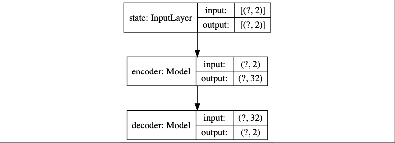
Figure 10.6.2: Autoencoder model
In Figure 10.6.3, the encoder is an MLP made of Input(2)-Dense(256, activation='relu')-Dense(128, activation='relu')-Dense(32). Every state is converted into a 32-dim feature vector:
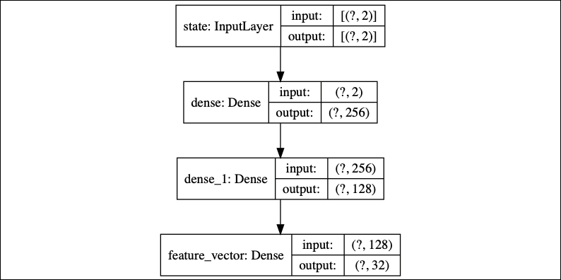
Figure 10.6.3: Encoder model
In Figure 10.6.4, the decoder is also an MLP but made of Input(32)-Dense(128, activation='relu')-Dense(256, activation='relu')-Dense(2):
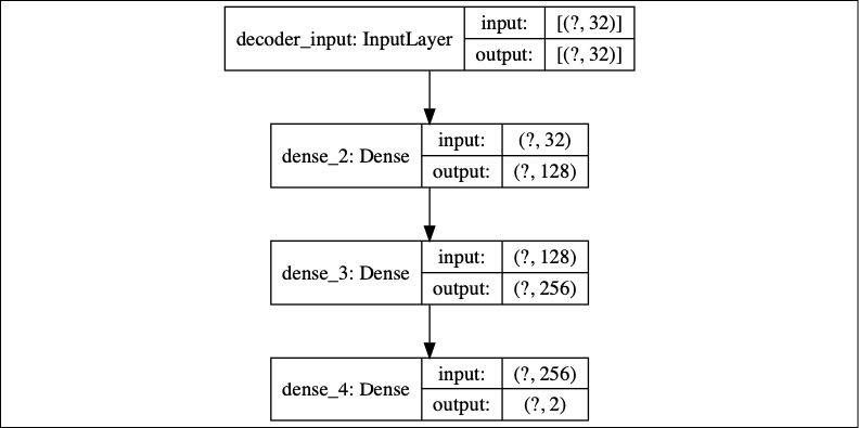
Figure 10.6.4: Decoder model
The autoencoder is trained for 10 epochs with an MSE, loss function, and tf.keras default Adam optimizer. We sampled 220,000 random states for the training and test dataset and applied a 200,000/20,000 train-test split. After training, the encoder weights are saved for future use in the policy and value networks' training. Listing 10.6.1 shows the methods for building and training the autoencoder.
In the tf.keras implementation, all the routines that we will mention in this section are implemented as methods in the PolicyAgent class unless otherwise noted. The role of PolicyAgent is to represent policy gradient methods' common functionalities, including building and training the autoencoder network model and predicting the action, log probability, entropy, and state value. This is the super class of each policy gradient method agent class presented in Listing 10.2.1 to Listing 10.5.1.
Listing 10.6.1: policygradient-car-10.1.1.py
Methods for building and training the feature autoencoder:
class PolicyAgent:
    def __init__(self, env):
        """Implements the models and training of
            Policy Gradient Methods
        Argument:
            env (Object): OpenAI gym environment
        """
        self.env = env
        # entropy loss weight
        self.beta = 0.0
        # value loss for all policy gradients except A2C
        self.loss = self.value_loss
        # s,a,r,s' are stored in memory
        self.memory = []
        # for computation of input size
        self.state = env.reset()
        self.state_dim = env.observation_space.shape[0]
        self.state = np.reshape(self.state, [1, self.state_dim])
        self.build_autoencoder()
    def build_autoencoder(self):
        """autoencoder to convert states into features
        """
        # first build the encoder model
        inputs = Input(shape=(self.state_dim, ), name='state')
        feature_size = 32
        x = Dense(256, activation='relu')(inputs)
        x = Dense(128, activation='relu')(x)
        feature = Dense(feature_size, name='feature_vector')(x)
        # instantiate encoder model
        self.encoder = Model(inputs, feature, name='encoder')
        self.encoder.summary()
        plot_model(self.encoder,
                   to_file='encoder.png',
                   show_shapes=True)
        # build the decoder model
        feature_inputs = Input(shape=(feature_size,),
                               name='decoder_input')
        x = Dense(128, activation='relu')(feature_inputs)
        x = Dense(256, activation='relu')(x)
        outputs = Dense(self.state_dim, activation='linear')(x)
        # instantiate decoder model
        self.decoder = Model(feature_inputs,
                             outputs,
                             name='decoder')
        self.decoder.summary()
        plot_model(self.decoder,
                   to_file='decoder.png',
                   show_shapes=True)
        # autoencoder = encoder + decoder
        # instantiate autoencoder model
        self.autoencoder = Model(inputs,
                                 self.decoder(self.encoder(inputs)),
                                 name='autoencoder')
        self.autoencoder.summary()
        plot_model(self.autoencoder,
                   to_file='autoencoder.png',
                   show_shapes=True)
        # Mean Square Error (MSE) loss function, Adam optimizer
        self.autoencoder.compile(loss='mse', optimizer='adam')
    def train_autoencoder(self, x_train, x_test):
        """Training the autoencoder using randomly sampled
            states from the environment
        Arguments:
            x_train (tensor): autoencoder train dataset
            x_test (tensor): autoencoder test dataset
        """
        # train the autoencoder
        batch_size = 32
        self.autoencoder.fit(x_train,
                             x_train,
                             validation_data=(x_test, x_test),
                             epochs=10,
                             batch_size=batch_size)
Given the MountainCarContinuous-v0 environment, the policy (or actor) model predicts the action that must be applied to the car. As discussed in the first section of this chapter on policy gradient methods, for continuous action spaces, the policy model samples an action from a Gaussian distribution, ![]() . In
. In tf.keras, this is implemented as:
import tensorflow_probability as tfp
    def action(self, args):
        """Given mean and stddev, sample an action, clip
            and return
            We assume Gaussian distribution of probability
            of selecting an action given a state
        Arguments:
            args (list) : mean, stddev list
        """
        mean, stddev = args
        dist = tfp.distributions.Normal(loc=mean, scale=stddev)
        action = dist.sample(1)
        action = K.clip(action,
                        self.env.action_space.low[0],
                        self.env.action_space.high[0])
        return action
The action is clipped between its minimum and maximum possible values. In this method, we use the TensorFlow probability package. It can be installed separately by:
pip3 install --upgrade tensorflow-probability
The role of the policy network is to predict the mean and standard deviation of the Gaussian distribution. Figure 10.6.5 shows the policy network to model ![]() .
.
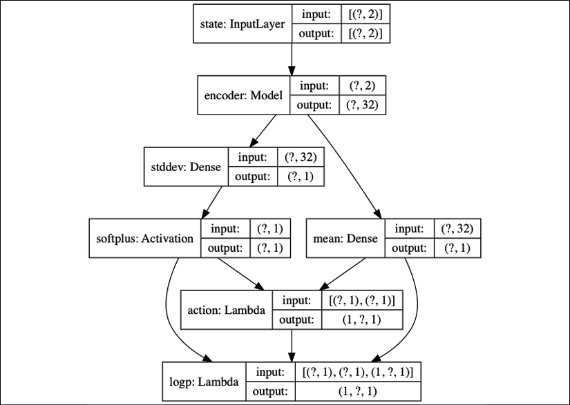
Figure 10.6.5: Policy model (actor model)
Note that the encoder model has pretrained weights that are frozen. Only the mean and standard deviation weights receive the performance gradient updates. The policy network is basically the implementation of Equation 10.1.4 and Equation 10.1.5, which are repeated here for convenience:
 (Equation 10.1.4) (Equation 10.1.5)
where ![]() is the encoder,
is the encoder, ![]() are the weights of the mean's
are the weights of the mean's Dense(1) layer, and ![]() are the weights of the standard deviation's
are the weights of the standard deviation's Dense(1) layer. We used a modified softplus function, ![]() , to avoid zero standard deviation:
, to avoid zero standard deviation:
def softplusk(x):
    """Some implementations use a modified softplus
        to ensure that the stddev is never zero
    Argument:
        x (tensor): activation input
    """
    return K.softplus(x) + 1e-10
The policy model builder is shown in Listing 10.6.2. Also included in this listing are the log probability, entropy, and value models, which we will discuss next.
Listing 10.6.2: policygradient-car-10.1.1.py
Method for building the policy (actor), logp, entropy, and value models from the encoded state features:
    def build_actor_critic(self):
        """4 models are built but 3 models share the
            same parameters. hence training one, trains the rest.
            The 3 models that share the same parameters
                are action, logp, and entropy models.
            Entropy model is used by A2C only.
            Each model has the same MLP structure:
            Input(2)-Encoder-Output(1).
            The output activation depends on the nature
                of the output.
        """
        inputs = Input(shape=(self.state_dim, ), name='state')
        self.encoder.trainable = False
        x = self.encoder(inputs)
        mean = Dense(1,
                     activation='linear',
                     kernel_initializer='zero',
                     name='mean')(x)
        stddev = Dense(1,
                       kernel_initializer='zero',
                       name='stddev')(x)
        # use of softplusk avoids stddev = 0
        stddev = Activation('softplusk', name='softplus')(stddev)
        action = Lambda(self.action,
                        output_shape=(1,),
                        name='action')([mean, stddev])
        self.actor_model = Model(inputs, action, name='action')
        self.actor_model.summary()
        plot_model(self.actor_model,
                   to_file='actor_model.png',
                   show_shapes=True)
        logp = Lambda(self.logp,
                      output_shape=(1,),
                      name='logp')([mean, stddev, action])
        self.logp_model = Model(inputs, logp, name='logp')
        self.logp_model.summary()
        plot_model(self.logp_model,
                   to_file='logp_model.png',
                   show_shapes=True)
        entropy = Lambda(self.entropy,
                         output_shape=(1,),
                         name='entropy')([mean, stddev])
        self.entropy_model = Model(inputs, entropy, name='entropy')
        self.entropy_model.summary()
        plot_model(self.entropy_model,
                   to_file='entropy_model.png',
                   show_shapes=True)
        value = Dense(1,
                      activation='linear',
                      kernel_initializer='zero',
                      name='value')(x)
        self.value_model = Model(inputs, value, name='value')
        self.value_model.summary()
        plot_model(self.value_model,
                   to_file='value_model.png',
                   show_shapes=True)
        # logp loss of policy network
        loss = self.logp_loss(self.get_entropy(self.state),
                              beta=self.beta)
        optimizer = RMSprop(lr=1e-3)
        self.logp_model.compile(loss=loss, optimizer=optimizer)
        optimizer = Adam(lr=1e-3)
        self.value_model.compile(loss=self.loss, optimizer=optimizer)

Figure 10.6.6: Gaussian log probability model of the policy
Apart from the policy network, ![]() , we must also have the action log probability (
, we must also have the action log probability (logp) network ![]() , since this is actually the one that calculates the gradient. As shown in Figure 10.6.6, the
, since this is actually the one that calculates the gradient. As shown in Figure 10.6.6, the logp network is simply the policy network where an additional Lambda(1) layer computes the log probability of the Gaussian distribution given the action, mean, and standard deviation.
The logp network and actor (policy) model share the same set of parameters. The Lambda layer does not have any parameters. It is implemented by the following function:
    def logp(self, args):
        """Given mean, stddev, and action compute
            the log probability of the Gaussian distribution
        Arguments:
            args (list) : mean, stddev action, list
        """
        mean, stddev, action = args
        dist = tfp.distributions.Normal(loc=mean, scale=stddev)
        logp = dist.log_prob(action)
        return logp
Training the logp network trains the actor model as well. In the training methods that are discussed in this section, only the logp network is trained.
As shown in Figure 10.6.7, the entropy model also shares parameters with the policy network:

Figure 10.6.7: Entropy model
The output Lambda(1) layer computes the entropy of the Gaussian distribution given the mean and standard deviation using the following function:
    def entropy(self, args):
        """Given the mean and stddev compute
            the Gaussian dist entropy
        Arguments:
            args (list) : mean, stddev list
        """
        mean, stddev = args
        dist = tfp.distributions.Normal(loc=mean, scale=stddev)
        entropy = dist.entropy()
        return entropy
The entropy model is only used by the A2C method.
Figure 10.6.8 shows the value model:

Figure 10.6.8: A value model
The model also uses the pretrained encoder with frozen weights to implement the following equation, Equation 10.3.2, which is repeated here for convenience:
 (Equation 10.3.2)
![]() are the weights of the
are the weights of the Dense(1) layer, the only layer that receives value gradient updates. Figure 10.6.8 represents ![]() in Algorithm 10.3.1 to Algorithm 10.5.1. The value model can be built in a few lines:
in Algorithm 10.3.1 to Algorithm 10.5.1. The value model can be built in a few lines:
inputs = Input(shape=(self.state_dim, ), name='state')
self.encoder.trainable = False
x = self.encoder(inputs)
value = Dense(1,
              activation='linear',
              kernel_initializer='zero',
              name='value')(x)
self.value_model = Model(inputs, value, name='value')
These lines are also implemented in the build_actor_critic() method, which is shown in Listing 10.6.2.
After building the network models, the next step is training. In Algorithm 10.2.1 to Algorithm 10.5.1, we perform objective function maximization by gradient ascent. In tf.keras, we perform loss function minimization by gradient descent. The loss function is simply the negative of the objective function being maximized. The gradient descent is the negative of gradient ascent. Listing 10.6.3 shows the logp and value loss functions.
We can take advantage of the common structure of the loss functions to unify the loss functions in Algorithm 10.2.1 to Algorithm 10.5.1. The performance and value gradients differ only in their constant factors. All performance gradients have the common term, ![]() . This is represented by
. This is represented by y_pred in the policy log probability loss function, logp_loss(). The factor to the common term, ![]() , depends on which algorithm and is implemented as
, depends on which algorithm and is implemented as y_true. Table 10.6.1 shows the values of y_true. The remaining term is the weighted gradient of entropy, ![]() . This is implemented as the product of
. This is implemented as the product of beta and entropy in the logp_loss() function. Only A2C uses this term, so, by default, self.beta=0.0. For A2C, self.beta=0.9.
Listing 10.6.3: policygradient-car-10.1.1.py
Loss functions of the logp and value networks:
    def logp_loss(self, entropy, beta=0.0):
        """logp loss, the 3rd and 4th variables
            (entropy and beta) are needed by A2C
            so we have a different loss function structure
        Arguments:
            entropy (tensor): Entropy loss
            beta (float): Entropy loss weight
        """
        def loss(y_true, y_pred):
            return -K.mean((y_pred * y_true)
                    + (beta * entropy), axis=-1)
return loss
    def value_loss(self, y_true, y_pred):
        """Typical loss function structure that accepts
            2 arguments only
           this will be used by value loss of all methods
            except A2C
        Arguments:
            y_true (tensor): value ground truth
            y_pred (tensor): value prediction
        """
        return -K.mean(y_pred * y_true, axis=-1)
| Algorithm | y_true of logp_loss | y_true of value_loss |
|
10.2.1 REINFORCE |
|
|
|
|
|
|
|
10.4.1 Actor-Critic |
|
|
|
10.5.1 A2C |
|
|
Table 10.6.1: y_true value of logp_loss and value_loss
The code implementation for computing y_true in Table 10.6.1 is shown in Table 10.6.2:
| Algorithm | y_true formula | y_true in Keras |
|
10.2.1 REINFORCE |
|
|
|
10.3.1 REINFORCE with baseline |
|
( |
|
10.4.1 Actor-Critic |
|
( + |
|
10.5.1 A2C |
and |
( and |
Table 10.6.2: y_true value in Table 10.6.1
Similarly, the value loss functions of Algorithm 10.3.1 and Algorithm 10.4.1 have the same structure. The value loss functions are implemented in tf.keras as value_loss(), as shown in Listing 10.6.3. The common gradient factor ![]() is represented by the tensor,
is represented by the tensor, y_pred. The remaining factor is represented by y_true. The y_true values are also shown in Table 10.6.1. REINFORCE does not use a value function. A2C uses the MSE loss function to learn the value function. In A2C, y_true represents the target value or ground truth.
With all the network models and loss functions in place, the last part is the training strategy, which is different for each algorithm. The training algorithm per policy gradient method has been discussed in Listing 10.2.1 to Listing 10.5.1. Algorithm 10.2.1, Algorithm 10.3.1, and Algorithm 10.5.1 wait for a complete episode to finish before training, so it runs both train_by_episode() and train(). The complete episode is saved in self.memory. Actor-Critic Algorithm 10.4.1 trains per step and only runs train().
Listing 10.6.4 shows how one episode unfolds when the agent executes and trains the policy and value models. The for loop is executed for 1,000 episodes. An episode terminates upon reaching 1,000 steps or when the car touches the flag. The agent executes the action predicted by the policy at every step. After each episode or step, the training routine is called.
Listing 10.6.4: policygradient-car-10.1.1.py
    # sampling and fitting
    for episode in range(episode_count):
        state = env.reset()
        # state is car [position, speed]
        state = np.reshape(state, [1, state_dim])
        # reset all variables and memory before the start of
        # every episode
        step = 0
        total_reward = 0
        done = False
        agent.reset_memory()
        while not done:
            # [min, max] action = [-1.0, 1.0]
            # for baseline, random choice of action will not move
            # the car pass the flag pole
            if args.random:
                action = env.action_space.sample()
            else:
                action = agent.act(state)
            env.render()
            # after executing the action, get s', r, done
            next_state, reward, done, _ = env.step(action)
            next_state = np.reshape(next_state, [1, state_dim])
            # save the experience unit in memory for training
            # Actor-Critic does not need this but we keep it anyway.
            item = [step, state, next_state, reward, done]
            agent.remember(item)
            if args.actor_critic and train:
                # only actor-critic performs online training
                # train at every step as it happens
                agent.train(item, gamma=0.99)
            elif not args.random and done and train:
                # for REINFORCE, REINFORCE with baseline, and A2C
                # we wait for the completion of the episode before
                # training the network(s)
                # last value as used by A2C
                if args.a2c:
                    v = 0 if reward > 0 else agent.value(next_state)[0]
                    agent.train_by_episode(last_value=v)
                else:
                    agent.train_by_episode()
            # accumulate reward
            total_reward += reward
            # next state is the new state
            state = next_state
            step += 1
During training, we collected data to determine the performance of each policy gradient algorithm. In the next section, we summarize the results.
7. Performance evaluation of policy gradient methods
The 4 policy gradients methods were evaluated by training the agent for 1,000 episodes. We define 1 training session as 1,000 episodes of training. The first performance metric is measured by accumulating the number of times the car reached the flag in 1,000 episodes.
In this metric, A2C reached the flag the greatest number of times, followed by REINFORCE with baseline, Actor-Critic, and REINFORCE. The use of baseline or critic accelerates the learning. Note that these are training sessions, where the agent is continuously improving its performance. There were cases in the experiments where the agent's performance did not improve with time.
The second performance metric is based on the requirement that MountainCarContinuous-v0 is considered solved if the total reward per episode is at least 90.0. From the 5 training sessions per method, we selected 1 training session with the highest total reward for the last 100 episodes (episodes 900 to 999).
Figure 10.7.1 to Figure 10.7.4 show the number of times the mountain car reached the flag during the execution of 1,000 episodes.

Figure 10.7.1: The number of times the mountain car reached the flag using the REINFORCE method

Figure 10.7.2: The number of times the mountain car reached the flag using the REINFORCE with baseline method

Figure 10.7.3: The number of times the mountain car reached the flag using the Actor-Critic method

Figure 10.7.4: The number of times the mountain car reached the flag using the A2C method
Figure 10.7.5 to Figure 10.7.8 show the total rewards for 1,000 episodes.

Figure 10.7.5: Total rewards received per episode using the REINFORCE method

Figure 10.7.6: Total rewards received per episode using the REINFORCE with baseline method.

Figure 10.7.7: Total rewards received per episode using the Actor-Critic method

Figure 10.7.8: The total rewards received per episode using the A2C method
REINFORCE with baseline is the only method that was able to consistently achieve a total reward of about 90 within 1,000 episodes of training. A2C has the second-best performance, but could not consistently reach at least 90 for the total rewards.
In the experiments conducted, we used the same learning rate, 1e-3, for log probability and value network optimization. The discount factor is set to 0.99, except for A2C, which is easier to train at a discount factor of 0.95.
The reader is encouraged to run the trained network by executing:
python3 policygradient-car-10.1.1.py
--encoder_weights=encoder_weights.h5 --actor_weights=actor_weights.h5
Table 10.7.1 shows other modes of running policygradient-car-10.1.1.py. The weights file (that is, *.h5) can be replaced by your own pretrained weights file. Please consult the code to see the other potential options.
| Purpose | Run |
|
Train REINFORCE from scratch |
|
|
Train REINFORCE with baseline from scratch |
|
|
Train Actor-Critic from scratch |
|
|
Train A2C from scratch |
|
|
Train REINFORCE from previously saved weights |
|
|
Train REINFORCE with baseline from previously saved weights |
|
|
Train Actor-Critic from previously saved weights |
|
|
Train A2C from previously saved weights |
|
Table 10.7.1: Different options in running policygradient-car-10.1.1.py
As a final note, our implementation of the policy gradient methods in tf.keras has some limitations. For example, training the actor model requires the action to be resampled. The action is first sampled and applied to the environment to observe the reward and next state. Then, another sample is taken to train the log probability model. The second sample is not necessarily the same as the first one, but the reward that is used for training comes from the first sampled action, which can introduce stochastic error in the computation of gradients.
8. Conclusion
In this chapter, we've covered the policy gradient methods. Starting with the policy gradient theorem, we formulated four methods to train the policy network. The four methods, REINFORCE, REINFORCE with baseline, Actor-Critic, and A2C algorithms, were discussed in detail. We explored how the four methods could be implemented in Keras. We then validated the algorithms by examining the number of times the agent successfully reached its goal and in terms of the total rewards received per episode.
Similar to the deep Q-network [2] that we discussed in the previous chapter, there are several improvements that can be done on the fundamental policy gradient algorithms. For example, the most prominent one is the A3C [3], which is a multithreaded version of A2C. This enables the agent to get exposed to different experiences simultaneously and to optimize the policy and value networks asynchronously. However, in the experiments conducted by OpenAI, https://blog.openai.com/baselines-acktr-a2c/, there is no strong advantage of A3C over A2C since the former could not take advantage of the strong GPUs available nowadays.
In the next two chapters, we will embark on a different area – object detection and semantic segmentation. Object detection enables an agent to identify and localize objects in a given image. Semantic segmentation identifies pixel regions in a given image based on object category.
9. References
- Richard Sutton and Andrew Barto: Reinforcement Learning: An Introduction: http://incompleteideas.net/book/bookdraft2017nov5.pdf (2017)
- Volodymyr Mnih et al.: Human-level control through deep reinforcement learning, Nature 518.7540 (2015): 529
- Volodymyr Mnih et al.: Asynchronous Methods for Deep Reinforcement Learning, International conference on machine learning, 2016
- Ronald Williams: Simple statistical gradient-following algorithms for connectionist reinforcement learning, Machine learning 8.3-4 (1992): 229-256