6
Disentangled Representation GANs
As we've explored, GANs can generate meaningful outputs by learning the data distribution. However, there was no control over the attributes of the generated outputs. Some variations of GANs, like conditional GAN (CGAN) and auxiliary classifier GAN (ACGAN), as discussed in the previous two chapters, are able to train a generator that is conditioned to synthesize specific outputs. For example, both CGAN and ACGAN can induce the generator to produce a specific MNIST digit. This is achieved by using both a 100-dim noise code and the corresponding one-hot label as inputs. However, other than the one-hot label, we have no other ways to control the properties of generated outputs.
For a review of CGAN and ACGAN, please refer to Chapter 4, Generative Adversarial Networks (GANs), and Chapter 5, Improved GANs.
In this chapter, we will be covering the variations of GANs that enable us to modify the generator outputs. In the context of the MNIST dataset, apart from which number to produce, we may find that we want to control the writing style. This could involve the tilt or the width of the desired digit. In other words, GANs can also learn disentangled latent codes or representations that we can use to vary the attributes of the generator outputs. A disentangled code or representation is a tensor that can change a specific feature or attribute of the output data while not affecting the other attributes.
In the first section of this chapter, we will be discussing InfoGAN: Interpretable Representation Learning by Information Maximizing Generative Adversarial Nets [1], an extension to GANs. InfoGAN learns the disentangled representations in an unsupervised manner by maximizing the mutual information between the input codes and the output observation. On the MNIST dataset, InfoGAN disentangles the writing styles from the digits dataset.
In the following part of the chapter, we'll also be discussing the Stacked Generative Adversarial Networks or StackedGAN [2], another extension to GANs.
StackedGAN uses a pretrained encoder or classifier in order to aid in disentangling the latent codes. StackedGAN can be viewed as a stack of models, with each being made of an encoder and a GAN. Each GAN is trained in an adversarial manner by using the input and output data of the corresponding encoder.
In summary, the goal of this chapter is to present:
- The concepts of disentangled representations
- The principles of both InfoGAN and StackedGAN
- Implementation of both InfoGAN and StackedGAN using
tf.keras
Let's begin by discussing disentangled representations.
1. Disentangled representations
The original GAN was able to generate meaningful outputs, but the downside was that its attributes couldn't be controlled. For example, if we trained a GAN to learn a distribution of celebrity faces, the generator would produce new images of celebrity-looking people. However, there is no way to influence the generator regarding the specific attributes of the face that we want. For example, we're unable to ask the generator for a face of a female celebrity with long black hair, a fair complexion, brown eyes, and who is smiling. The fundamental reason for this is because the 100-dim noise code that we use entangles all of the salient attributes of the generator outputs. We can recall that in tf.keras, the 100-dim code was generated by the random sampling of uniform noise distribution:
        # generate fake images from noise using generator
        # generate noise using uniform distribution
        noise = np.random.uniform(-1.0,
                                  1.0,
                                  size=[batch_size, latent_size])
        # generate fake images
        fake_images = generator.predict(noise)
If we are able to modify the original GAN such that the representation is separated into entangled and disentangled interpretable latent code vectors, we would be able to tell the generator what to synthesize.
Figure 6.1.1 shows us a GAN with an entangled code and its variation with a mixture of entangled and disentangled representations. In the context of the hypothetical celebrity face generation, with the disentangled codes, we are able to indicate the gender, hairstyle, facial expression, skin complexion, and eye color of the face we wish to generate. The n–dim entangled code is still needed to represent all the other facial attributes that we have not disentangled, such as the face shape, facial hair, eye-glasses, as just three examples. The concatenation of entangled and disentangled code vectors serves as the new input to the generator. The total dimension of the concatenated code may not be necessarily 100:

Figure 6.1.1: The GAN with the entangled code and its variation with both entangled and disentangled codes. This example is shown in the context of celebrity face generation
Looking at the preceding figure, it appears that GANs with disentangled representations can also be optimized in the same way as a vanilla GAN can be. This is because the generator output can be represented as:
 (Equation 6.1.1)
The code z = (z, c) comprises two elements:
- Incompressible entangled noise code similar to GANs z or noise vector.
- Latent codes, c1,c2,…,cL, which represent the interpretable disentangled codes of the data distribution. Collectively, all latent codes are represented by c.
For simplicity, all the latent codes are assumed to be independent:
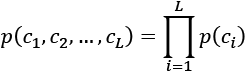 (Equation 6.1.2)
The generator function ![]() is provided with both the incompressible noise code and the latent codes. From the point of view of the generator, optimizing z = (z, c) is the same as optimizing z.
is provided with both the incompressible noise code and the latent codes. From the point of view of the generator, optimizing z = (z, c) is the same as optimizing z.
The generator network will simply ignore the constraint imposed by the disentangled codes when coming up with a solution.
The generator learns the distribution ![]() . This will practically defeat the objective of disentangled representations.
. This will practically defeat the objective of disentangled representations.
The key idea of InfoGAN is to force the GAN not to ignore the latent code c. This is done by maximizing the mutual information between c and ![]() . In the next section, we will formulate the loss function of InfoGAN.
. In the next section, we will formulate the loss function of InfoGAN.
InfoGAN
To enforce the disentanglement of codes, InfoGAN proposed a regularizer to the original loss function that maximizes the mutual information between the latent codes c and ![]() :
:
 (Equation 6.1.3)
The regularizer forces the generator to consider the latent codes when it formulates a function that synthesizes the fake images. In the field of information theory, the mutual information between latent codes c and ![]() is defined as:
is defined as:
 (Equation 6.1.4)
Where H(c) is the entropy of latent code, c, and ![]() is the conditional entropy of c after observing the output of the generator,
is the conditional entropy of c after observing the output of the generator, ![]() . Entropy is a measure of uncertainty of a random variable or an event. For example, information such as the sun rises in the east has a low entropy, whereas winning the jackpot in the lottery has a high entropy. A more detailed discussion on mutual information can be found in Chapter 13, Unsupervised Learning Using Mutual Information.
. Entropy is a measure of uncertainty of a random variable or an event. For example, information such as the sun rises in the east has a low entropy, whereas winning the jackpot in the lottery has a high entropy. A more detailed discussion on mutual information can be found in Chapter 13, Unsupervised Learning Using Mutual Information.
In Equation 6.1.4, maximizing the mutual information means minimizing ![]() or decreasing the uncertainty in the latent code upon observing the generated output. This makes sense since, for example, in the MNIST dataset, the generator becomes more confident in synthesizing the digit 8 if the GAN sees that it observed the digit 8.
or decreasing the uncertainty in the latent code upon observing the generated output. This makes sense since, for example, in the MNIST dataset, the generator becomes more confident in synthesizing the digit 8 if the GAN sees that it observed the digit 8.
However, it is hard to estimate ![]() since it requires knowledge of the posterior
since it requires knowledge of the posterior ![]() , which is something that we don't have access to. For simplicity, we will use the regular letter x to represent the data distribution.
, which is something that we don't have access to. For simplicity, we will use the regular letter x to represent the data distribution.
The workaround is to estimate the lower bound of mutual information by estimating the posterior with an auxiliary distribution ![]() . InfoGAN estimates the lower bound of mutual information as:
. InfoGAN estimates the lower bound of mutual information as:
 (Equation 6.1.5)
In InfoGAN, H(c) is assumed to be a constant. Therefore, maximizing the mutual information is a matter of maximizing the expectation. The generator must be confident that it has generated an output with the specific attributes. We should note that the maximum value of this expectation is zero. Therefore, the maximum of the lower bound of the mutual information is H(c). In InfoGAN, ![]() for discrete latent codes can be represented by
for discrete latent codes can be represented by softmax nonlinearity. The expectation is the negative categorical_crossentropy loss in tf.keras.
For continuous codes of a single dimension, the expectation is a double integral over c and x. This is due to the expectation that samples from both disentangled code distribution and generator distribution. One way of estimating the expectation is by assuming the samples as a good measure of continuous data. Therefore, the loss is estimated as ![]() . In Chapter 13, Unsupervised Learning Using Mutual Information, we will present a more precise estimation of mutual information.
. In Chapter 13, Unsupervised Learning Using Mutual Information, we will present a more precise estimation of mutual information.
To complete the network of an InfoGAN, we should have an implementation of ![]() . For simplicity, the network Q is an auxiliary network attached to the second to last layer of the discriminator. Therefore, this has a minimal impact on the training of the original GAN.
. For simplicity, the network Q is an auxiliary network attached to the second to last layer of the discriminator. Therefore, this has a minimal impact on the training of the original GAN.
Figure 6.1.2 shows the InfoGAN network diagram:

Figure 6.1.2 Network diagram showing discriminator and generator training in InfoGAN
Table 6.1.1 shows the loss functions of InfoGAN as compared to GAN:
| Network | Loss Functions | Number |
|
GAN |
|
4.1.1 4.1.5 |
|
InfoGAN |
For continuous codes, InfoGAN recommends a value of |
6.1.1 6.1.2 |
Table 6.1.1: A comparison between the loss functions of GAN and InfoGAN
The loss functions of InfoGAN differ from GANs by an additional term, ![]() , where
, where ![]() is a small positive constant. Minimizing the loss function of an InfoGAN translates to minimizing the loss of the original GAN and maximizing the mutual information
is a small positive constant. Minimizing the loss function of an InfoGAN translates to minimizing the loss of the original GAN and maximizing the mutual information ![]() .
.
If applied to the MNIST dataset, InfoGAN can learn the disentangled discrete and continuous codes in order to modify the generator output attributes. For example, like CGAN and ACGAN, the discrete code in the form of a 10-dim one-hot label will be used to specify the digit to generate. However, we can add two continuous codes, one for controlling the angle of writing style and another for adjusting the stroke width. Figure 6.1.3 shows the codes for the MNIST digit in InfoGAN. We retain the entangled code with a smaller dimensionality to represent all other attributes:

Figure 6.1.3: The codes for both GAN and InfoGAN in the context of the MNIST dataset
Having discussed some of the concepts behind InfoGAN, let's take a look at InfoGAN implementation in tf.keras.
Implementation of InfoGAN in Keras
To implement an InfoGAN on the MNIST dataset, there are some changes that need to be made in the base code of the ACGAN. As highlighted in Listing 6.1.1, the generator concatenates both entangled (z noise code) and disentangled codes (one-hot label and continuous codes) to serve as input:
inputs = [inputs, labels] + codes
The builder functions for the generator and discriminator are also implemented in gan.py in the lib folder.
The complete code is available on GitHub: https://github.com/PacktPublishing/Advanced-Deep-Learning-with-Keras.
Listing 6.1.1: infogan-mnist-6.1.1.py
Highlighted are the lines that are specific to InfoGAN:
def generator(inputs,
              image_size,
              activation='sigmoid',
              labels=None,
              codes=None):
    """Build a Generator Model
    Stack of BN-ReLU-Conv2DTranpose to generate fake images.
    Output activation is sigmoid instead of tanh in [1].
    Sigmoid converges easily.
    Arguments:
        inputs (Layer): Input layer of the generator (the z-vector)
        image_size (int): Target size of one side
            (assuming square image)
        activation (string): Name of output activation layer
        labels (tensor): Input labels
        codes (list): 2-dim disentangled codes for InfoGAN
    Returns:
        Model: Generator Model
    """
    image_resize = image_size // 4
    # network parameters
    kernel_size = 5
    layer_filters = [128, 64, 32, 1]
    if labels is not None:
        if codes is None:
            # ACGAN labels
            # concatenate z noise vector and one-hot labels
            inputs = [inputs, labels]
        else:
            # infoGAN codes
            # concatenate z noise vector,
            # one-hot labels and codes 1 & 2
            inputs = [inputs, labels] + codes
        x = concatenate(inputs, axis=1)
    elif codes is not None:
        # generator 0 of StackedGAN
        inputs = [inputs, codes]
        x = concatenate(inputs, axis=1)
    else:
        # default input is just 100-dim noise (z-code)
        x = inputs
    x = Dense(image_resize * image_resize * layer_filters[0])(x)
    x = Reshape((image_resize, image_resize, layer_filters[0]))(x)
    for filters in layer_filters:
        # first two convolution layers use strides = 2
        # the last two use strides = 1
        if filters > layer_filters[-2]:
            strides = 2
        else:
            strides = 1
        x = BatchNormalization()(x)
        x = Activation('relu')(x)
        x = Conv2DTranspose(filters=filters,
                            kernel_size=kernel_size,
                            strides=strides,
                            padding='same')(x)
    if activation is not None:
        x = Activation(activation)(x)
    # generator output is the synthesized image x
    return Model(inputs, x, name='generator')
Listing 6.1.2 shows the discriminator and Q network with the original default GAN output. The three auxiliary outputs corresponding to discrete code (for one-hot label) softmax prediction and the continuous code probabilities given the input MNIST digit image are highlighted.
Listing 6.1.2: infogan-mnist-6.1.1.py
Highlighted are the lines that are specific to InfoGAN:
def discriminator(inputs,
                  activation='sigmoid',
                  num_labels=None,
                  num_codes=None):
    """Build a Discriminator Model
    Stack of LeakyReLU-Conv2D to discriminate real from fake
    The network does not converge with BN so it is not used here
    unlike in [1]
    Arguments:
        inputs (Layer): Input layer of the discriminator (the image)
        activation (string): Name of output activation layer
        num_labels (int): Dimension of one-hot labels for ACGAN & InfoGAN
        num_codes (int): num_codes-dim Q network as output
                    if StackedGAN or 2 Q networks if InfoGAN
    Returns:
        Model: Discriminator Model
    """
    kernel_size = 5
    layer_filters = [32, 64, 128, 256]
    x = inputs
    for filters in layer_filters:
        # first 3 convolution layers use strides = 2
        # last one uses strides = 1
        if filters == layer_filters[-1]:
            strides = 1
        else:
            strides = 2
        x = LeakyReLU(alpha=0.2)(x)
        x = Conv2D(filters=filters,
                   kernel_size=kernel_size,
                   strides=strides,
                   padding='same')(x)
    x = Flatten()(x)
    # default output is probability that the image is real
    outputs = Dense(1)(x)
    if activation is not None:
        print(activation)
        outputs = Activation(activation)(outputs)
    if num_labels:
        # ACGAN and InfoGAN have 2nd output
        # 2nd output is 10-dim one-hot vector of label
        layer = Dense(layer_filters[-2])(x)
        labels = Dense(num_labels)(layer)
        labels = Activation('softmax', name='label')(labels)
        if num_codes is None:
            outputs = [outputs, labels]
        else:
            # InfoGAN have 3rd and 4th outputs
            # 3rd output is 1-dim continous Q of 1st c given x
            code1 = Dense(1)(layer)
            code1 = Activation('sigmoid', name='code1')(code1)
            # 4th output is 1-dim continuous Q of 2nd c given x
            code2 = Dense(1)(layer)
            code2 = Activation('sigmoid', name='code2')(code2)
            outputs = [outputs, labels, code1, code2]
    elif num_codes is not None:
        # StackedGAN Q0 output
        # z0_recon is reconstruction of z0 normal distribution
        z0_recon =  Dense(num_codes)(x)
        z0_recon = Activation('tanh', name='z0')(z0_recon)
        outputs = [outputs, z0_recon]
return Model(inputs, outputs, name='discriminator')
Figure 6.1.4 shows the InfoGAN model in tf.keras:

Figure 6.1.4: The InfoGAN Keras model
Building the discriminator and adversarial models also requires a number of changes. The changes are on the loss functions used. The original discriminator loss function, binary_crossentropy, the categorical_crossentropy for discrete code, and the mi_loss function for each continuous code comprise the overall loss function. Each loss function is given a weight of 1.0, except for the mi_loss function, which is given 0.5, corresponding to ![]() for the continuous code.
for the continuous code.
Listing 6.1.3 highlights the changes made. However, we should note that by using the builder function, the discriminator is instantiated as:
    # call discriminator builder with 4 outputs:
    # source, label, and 2 codes
    discriminator = gan.discriminator(inputs,
                                      num_labels=num_labels,
                                      num_codes=2)
    # call generator with inputs,
    # labels and codes as total inputs to generator
    generator = gan.generator(inputs,
                              image_size,
                              labels=labels,
                              codes=[code1, code2])
Listing 6.1.3: infogan-mnist-6.1.1.py
Mutual information loss function as well as building and training the InfoGAN discriminator and adversarial networks is demonstrated in the following code:
def mi_loss(c, q_of_c_given_x):
    """ Mutual information, Equation 5 in [2],
        assuming H(c) is constant
    """
    # mi_loss = -c * log(Q(c|x))
    return K.mean(-K.sum(K.log(q_of_c_given_x + K.epsilon()) * c,
                               axis=1))
def build_and_train_models(latent_size=100):
    """Load the dataset, build InfoGAN discriminator,
    generator, and adversarial models.
    Call the InfoGAN train routine.
    """
    # load MNIST dataset
    (x_train, y_train), (_, _) = mnist.load_data()
    # reshape data for CNN as (28, 28, 1) and normalize
    image_size = x_train.shape[1]
    x_train = np.reshape(x_train, [-1, image_size, image_size, 1])
    x_train = x_train.astype('float32') / 255
    # train labels
    num_labels = len(np.unique(y_train))
    y_train = to_categorical(y_train)
    model_name = "infogan_mnist"
    # network parameters
    batch_size = 64
    train_steps = 40000
    lr = 2e-4
    decay = 6e-8
    input_shape = (image_size, image_size, 1)
    label_shape = (num_labels, )
    code_shape = (1, )
    # build discriminator model
    inputs = Input(shape=input_shape, name='discriminator_input')
    # call discriminator builder with 4 outputs:
    # source, label, and 2 codes
    discriminator = gan.discriminator(inputs,
                                      num_labels=num_labels,
                                      num_codes=2)
    # [1] uses Adam, but discriminator converges easily with RMSprop
    optimizer = RMSprop(lr=lr, decay=decay)
    # loss functions: 1) probability image is real
    # (binary crossentropy)
    # 2) categorical cross entropy image label,
    # 3) and 4) mutual information loss
    loss = ['binary_crossentropy',
            'categorical_crossentropy',
            mi_loss,
            mi_loss]
    # lamda or mi_loss weight is 0.5
    loss_weights = [1.0, 1.0, 0.5, 0.5]
    discriminator.compile(loss=loss,
                          loss_weights=loss_weights,
                          optimizer=optimizer,
                          metrics=['accuracy'])
    discriminator.summary()
    # build generator model
    input_shape = (latent_size, )
    inputs = Input(shape=input_shape, name='z_input')
    labels = Input(shape=label_shape, name='labels')
    code1 = Input(shape=code_shape, name="code1")
    code2 = Input(shape=code_shape, name="code2")
    # call generator with inputs,
    # labels and codes as total inputs to generator
    generator = gan.generator(inputs,
                              image_size,
                              labels=labels,
                              codes=[code1, code2])
    generator.summary()
    # build adversarial model = generator + discriminator
    optimizer = RMSprop(lr=lr*0.5, decay=decay*0.5)
    discriminator.trainable = False
    # total inputs = noise code, labels, and codes
    inputs = [inputs, labels, code1, code2]
    adversarial = Model(inputs,
                        discriminator(generator(inputs)),
                        name=model_name)
    # same loss as discriminator
    adversarial.compile(loss=loss,
                        loss_weights=loss_weights,
                        optimizer=optimizer,
                        metrics=['accuracy'])
    adversarial.summary()
    # train discriminator and adversarial networks
    models = (generator, discriminator, adversarial)
    data = (x_train, y_train)
    params = (batch_size,
              latent_size,
              train_steps,
              num_labels,
              model_name)
    train(models, data, params)
As far as the training is concerned, we can see that the InfoGAN is similar to ACGAN, except that we need to supply c for the continuous code. c is drawn from normal distribution with a standard deviation of 0.5 and a mean of 0.0. We'll use randomly sampled labels for the fake data and dataset class labels for the real data to represent discrete latent code.
Listing 6.1.4 highlights the changes made to the training function. Similar to all previous GANs, the discriminator and generator (through adversarial training) are alternately trained. During adversarial training, the discriminator weights are frozen.
Sample generator output images are saved every 500 interval steps by using the gan.py plot_images() function.
Listing 6.1.4: infogan-mnist-6.1.1.py
def train(models, data, params):
    """Train the Discriminator and Adversarial networks
    Alternately train discriminator and adversarial networks by batch.
    Discriminator is trained first with real and fake images,
    corresponding one-hot labels and continuous codes.
    Adversarial is trained next with fake images pretending
    to be real, corresponding one-hot labels and continous codes.
    Generate sample images per save_interval.
    # Arguments
        models (Models): Generator, Discriminator, Adversarial models
        data (tuple): x_train, y_train data
        params (tuple): Network parameters
    """
    # the GAN models
    generator, discriminator, adversarial = models
    # images and their one-hot labels
    x_train, y_train = data
    # network parameters
    batch_size, latent_size, train_steps, num_labels, model_name =
            params
    # the generator image is saved every 500 steps
    save_interval = 500
    # noise vector to see how the generator output
    # evolves during training
    noise_input = np.random.uniform(-1.0,
                                    1.0,
                                    size=[16, latent_size])
    # random class labels and codes
    noise_label = np.eye(num_labels)[np.arange(0, 16) % num_labels]
    noise_code1 = np.random.normal(scale=0.5, size=[16, 1])
    noise_code2 = np.random.normal(scale=0.5, size=[16, 1])
    # number of elements in train dataset
    train_size = x_train.shape[0]
    print(model_name,
          "Labels for generated images: ",
          np.argmax(noise_label, axis=1))
    for i in range(train_steps):
        # train the discriminator for 1 batch
        # 1 batch of real (label=1.0) and fake images (label=0.0)
        # randomly pick real images and
        # corresponding labels from dataset
        rand_indexes = np.random.randint(0,
                                         train_size,
                                         size=batch_size)
        real_images = x_train[rand_indexes]
        real_labels = y_train[rand_indexes]
        # random codes for real images
        real_code1 = np.random.normal(scale=0.5,
                                      size=[batch_size, 1])
        real_code2 = np.random.normal(scale=0.5,
                                      size=[batch_size, 1])
        # generate fake images, labels and codes
        noise = np.random.uniform(-1.0,
                                  1.0,
                                  size=[batch_size, latent_size])
        fake_labels = np.eye(num_labels)[np.random.choice(num_labels,
                                                          batch_size)]
        fake_code1 = np.random.normal(scale=0.5,
                                      size=[batch_size, 1])
        fake_code2 = np.random.normal(scale=0.5,
                                      size=[batch_size, 1])
        inputs = [noise, fake_labels, fake_code1, fake_code2]
        fake_images = generator.predict(inputs)
        # real + fake images = 1 batch of train data
        x = np.concatenate((real_images, fake_images))
        labels = np.concatenate((real_labels, fake_labels))
        codes1 = np.concatenate((real_code1, fake_code1))
        codes2 = np.concatenate((real_code2, fake_code2))
        # label real and fake images
        # real images label is 1.0
        y = np.ones([2 * batch_size, 1])
        # fake images label is 0.0
        y[batch_size:, :] = 0
        # train discriminator network,
        # log the loss and label accuracy
        outputs = [y, labels, codes1, codes2]
        # metrics = ['loss', 'activation_1_loss', 'label_loss',
        # 'code1_loss', 'code2_loss', 'activation_1_acc',
        # 'label_acc', 'code1_acc', 'code2_acc']
        # from discriminator.metrics_names
        metrics = discriminator.train_on_batch(x, outputs)
        fmt = "%d: [discriminator loss: %f, label_acc: %f]"
        log = fmt % (i, metrics[0], metrics[6])
        # train the adversarial network for 1 batch
        # 1 batch of fake images with label=1.0 and
        # corresponding one-hot label or class + random codes
        # since the discriminator weights are frozen
        # in adversarial network only the generator is trained
        # generate fake images, labels and codes
        noise = np.random.uniform(-1.0,
                                  1.0,
                                  size=[batch_size, latent_size])
        fake_labels = np.eye(num_labels)[np.random.choice(num_labels,
                                                          batch_size)]
        fake_code1 = np.random.normal(scale=0.5,
                                      size=[batch_size, 1])
        fake_code2 = np.random.normal(scale=0.5,
                                      size=[batch_size, 1])
        # label fake images as real
        y = np.ones([batch_size, 1])
        # train the adversarial network
        # note that unlike in discriminator training,
        # we do not save the fake images in a variable
        # the fake images go to the discriminator
        # input of the adversarial for classification
        # log the loss and label accuracy
        inputs = [noise, fake_labels, fake_code1, fake_code2]
        outputs = [y, fake_labels, fake_code1, fake_code2]
        metrics  = adversarial.train_on_batch(inputs, outputs)
        fmt = "%s [adversarial loss: %f, label_acc: %f]"
        log = fmt % (log, metrics[0], metrics[6])
        print(log)
        if (i + 1) % save_interval == 0:
            # plot generator images on a periodic basis
            gan.plot_images(generator,
                            noise_input=noise_input,
                            noise_label=noise_label,
                            noise_codes=[noise_code1, noise_code2],
                            show=False,
                            step=(i + 1),
                            model_name=model_name)
    # save the model after training the generator
    # the trained generator can be reloaded for
    # future MNIST digit generation
    generator.save(model_name + ".h5")
Given the tf.keras implementation of InfoGAN, the next section presents the generator MNIST outputs with disentangled attributes.
Generator outputs of InfoGAN
Similar to all previous GANs that have been presented to us, we've trained our InfoGAN for 40,000 steps. After the training is completed, we're able to run the InfoGAN generator to generate new outputs using the model saved on the infogan_mnist.h5 file. The following validations are conducted:
- Generate digits 0 to 9 by varying the discrete labels from 0 to 9. Both continuous codes are set to zero. The results are shown in Figure 6.1.5. We can see that the InfoGAN discrete code can control the digits produced by the generator:
python3 infogan-mnist-6.1.1.py --generator=infogan_mnist.h5
--digit=0 --code1=0 --code2=0
to
python3 infogan-mnist-6.1.1.py --generator=infogan_mnist.h5
--digit=9 --code1=0 --code2=0
In Figure 6.1.5 we can see the images generated by the InfoGAN:

Figure 6.1.5: The images generated by the InfoGAN as the discrete code is varied from 0 to 9. Both continuous codes are set to zero
- Examine the effect of the first continuous code to understand which attribute has been affected. We vary the first continuous code from -2.0 to 2.0 for digits 0 to 9. The second continuous code is set to 0.0. Figure 6.1.6 shows that the first continuous code controls the thickness of the digit:
python3 infogan-mnist-6.1.1.py --generator=infogan_mnist.h5
--digit=0 --code1=0 --code2=0 --p1
Figure 6.1.6: The images generated by InfoGAN as the first continuous code is varied from -2.0 to 2.0 for digits 0 to 9. The second continuous code is set to zero. The first continuous code controls the thickness of the digit
- Similar to the previous step, but instead focusing more on the second continuous code. Figure 6.1.7 shows that the second continuous code controls the rotation angle (tilt) of the writing style:
python3 infogan-mnist-6.1.1.py --generator=infogan_mnist.h5
--digit=0 --code1=0 --code2=0 --p2

Figure 6.1.7: The images generated by InfoGAN as the second continuous code is varied from -2.0 to 2.0 for digits 0 to 9. The first continuous code is set to zero. The second continuous code controls the rotation angle (tilt) of the writing style
From these validation results, we can see that apart from the ability to generate MNIST-looking digits, InfoGAN expands the ability of conditional GANs such as CGAN and ACGAN. The network automatically learned two arbitrary codes that can control the specific attributes of the generator output. It would be interesting to see what additional attributes could be controlled if we increased the number of continuous codes beyond 2. This could be accomplished by augmenting the list of codes in the highlighted lines of Listing 6.1.1 to Listing 6.1.4.
The results in this section demonstrated that the attributes of the generator outputs can be disentangled by maximizing the mutual information between the code and the data distribution. In the following section, a different approach on disentanglement is presented. The idea of StackedGAN is to inject the code at the feature level.
2. StackedGAN
In the same spirit as InfoGAN, StackedGAN proposes a method for disentangling latent representations for conditioning generator outputs. However, StackedGAN uses a different approach to the problem. Instead of learning how to condition the noise to produce the desired output, StackedGAN breaks down a GAN into a stack of GANs. Each GAN is trained independently in the usual discriminator-adversarial manner with its own latent code.
Figure 6.2.1 shows us how StackedGAN works in the context of hypothetical celebrity face generation, assuming that the Encoder network has been trained to classify celebrity faces:

Figure 6.2.1: The basic idea of StackedGAN in the context of celebrity face generation. Assuming that there is a hypothetical deep encoder network that can perform classification on celebrity faces, a StackedGAN simply inverts the process of the encoder
The Encoder network is composed of a stack of simple encoders, Encoderi where i = 0 … n - 1 corresponding to n features. Each encoder extracts certain facial features. For example, Encoder0 may be the encoder for hairstyle features, Features1. All the simple encoders contribute to making the overall Encoder perform correct predictions.
The idea behind StackedGAN is that if we would like to build a GAN that generates fake celebrity faces, we should simply invert the Encoder. StackedGAN consists of a stack of simpler GANs, GANi where i = 0 … n - 1 corresponding to n features. Each GANi learns to invert the process of its corresponding encoder, Encoderi. For example, GAN0 generates fake celebrity faces from fake hairstyle features, which is the inverse of the Encoder0 process.
Each GANi uses a latent code, zi, that conditions its generator output. For example, the latent code, z0, can alter the hairstyle from curly to wavy. The stack of GANs can also act as one to synthesize fake celebrity faces, completing the inverse process of the whole Encoder. The latent code of each GANi, zi, can be used to alter specific attributes of fake celebrity faces.
With the key idea of how the StackedGAN works, let's proceed to the next section and see how it is implemented in tf.keras.
Implementation of StackedGAN in Keras
The detailed network model of a StackedGAN can be seen in Figure 6.2.2. For conciseness, only two encoder-GANs per stack are shown. The figure may initially appear complex, but it is just a repetition of an encoder-GAN, meaning that if we understood how to train one encoder-GAN, the remainder utilize the same concept.
In this section, we assume that the StackedGAN is designed for MNIST digit generation.

Figure 6.2.2: A StackedGAN comprises a stack of an encoder and a GAN. The encoder is pretrained to perform classification. Generator1, G1, learns to synthesize f1f features conditioned on the fake label, yf, and latent code, z1f. Generator0, G0, produces fake images using both the fake features, f1f and latent code, z0f
StackedGAN starts with an Encoder. It could be a trained classifier that predicts the correct labels. The intermediate features vector, f1r, is made available for GAN training. For MNIST, we can use a CNN-based classifier similar to what we discussed in Chapter 1, Introducing Advanced Deep Learning with Keras.
Figure 6.2.3 shows the Encoder and its network model implementation in tf.keras:

Figure 6.2.3: The encoder in StackedGAN is a simple CNN-based classifier
Listing 6.2.1 shows the tf.keras code for the preceding figure. It is similar to the CNN-based classifier in Chapter 1, Introducing Advanced Deep Learning with Keras, except that we use a Dense layer to extract the 256-dim feature. There are two output models, Encoder0 and Encoder1. Both will be used to train the StackedGAN.
Listing 6.2.1: stackedgan-mnist-6.2.1.py
def build_encoder(inputs, num_labels=10, feature1_dim=256):
    """ Build the Classifier (Encoder) Model sub networks
    Two sub networks:
    1) Encoder0: Image to feature1 (intermediate latent feature)
    2) Encoder1: feature1 to labels
    # Arguments
        inputs (Layers): x - images, feature1 -
            feature1 layer output
        num_labels (int): number of class labels
        feature1_dim (int): feature1 dimensionality
    # Returns
        enc0, enc1 (Models): Description below
    """
    kernel_size = 3
    filters = 64
    x, feature1 = inputs
    # Encoder0 or enc0
    y = Conv2D(filters=filters,
               kernel_size=kernel_size,
               padding='same',
               activation='relu')(x)
    y = MaxPooling2D()(y)
    y = Conv2D(filters=filters,
               kernel_size=kernel_size,
               padding='same',
               activation='relu')(y)
    y = MaxPooling2D()(y)
    y = Flatten()(y)
    feature1_output = Dense(feature1_dim, activation='relu')(y)
    # Encoder0 or enc0: image (x or feature0) to feature1
    enc0 = Model(inputs=x, outputs=feature1_output, name="encoder0")
    # Encoder1 or enc1
    y = Dense(num_labels)(feature1)
    labels = Activation('softmax')(y)
    # Encoder1 or enc1: feature1 to class labels (feature2)
    enc1 = Model(inputs=feature1, outputs=labels, name="encoder1")
    # return both enc0 and enc1
    return enc0, enc1
The Encoder0 output, f1r, is the 256-dim feature vector that we want Generator1 to learn to synthesize. It is available as an auxiliary output of Encoder0, E0. The overall Encoder is trained to classify MNIST digits, xr. The correct labels, yr, are predicted by Encoder1, E1. In the process, the intermediate set of features, f1r, is learned and made available for Generator0 training. Subscript r is used to emphasize and distinguish real data from fake data when the GAN is trained against this encoder.
Given that the Encoder inputs (xr) intermediate features (f1r) and labels (yr), each GAN is trained in the usual discriminator–adversarial manner. The loss functions are given by Equation 6.2.1 to Equation 6.2.5 in Table 6.2.1. Equation 6.2.1 and Equation 6.2.2 are the usual loss functions of the generic GAN. StackedGAN has two additional loss functions, Conditional and Entropy.
| Network | Loss Functions | Number |
|
GAN |
|
4.1.1 4.1.5 |
|
StackedGAN |
where |
6.2.1 6.2.2 6.2.3 6.2.4 6.2.5 |
Table 6.2.1: A comparison between the loss functions of GAN and StackedGAN. ~pdata means sampling from the corresponding encoder data (input, feature, or output)
The conditional loss function, ![]() in Equation 6.2.3, ensures that the generator does not ignore the input, fi+1, when synthesizing the output, fi, from the input noise code, zi. The encoder, Encoderi, must be able to recover the generator input by inverting the process of the generator, Generatori. The difference between the generator input and the recovered input using the encoder is measured by L2 or Euclidean distance (mean squared error (MSE)).
in Equation 6.2.3, ensures that the generator does not ignore the input, fi+1, when synthesizing the output, fi, from the input noise code, zi. The encoder, Encoderi, must be able to recover the generator input by inverting the process of the generator, Generatori. The difference between the generator input and the recovered input using the encoder is measured by L2 or Euclidean distance (mean squared error (MSE)).
Figure 6.2.4 shows the network elements involved in the computation of ![]() :
:

Figure 6.2.4: A simpler version of Figure 6.2.3 showing only the network elements involved in the computation of ![]()
The conditional loss function, however, introduces a new problem. The generator ignores the input noise code, zi and simply relies on fi+1. Entropy loss function, ![]() in Equation 6.2.4, ensures that the generator does not ignore the noise code, zi. The Q network recovers the noise code from the output of the generator. The difference between the recovered noise and the input noise is also measured by L2 or Euclidean distance (MSE).
in Equation 6.2.4, ensures that the generator does not ignore the noise code, zi. The Q network recovers the noise code from the output of the generator. The difference between the recovered noise and the input noise is also measured by L2 or Euclidean distance (MSE).
Figure 6.2.5 shows the network elements involved in the computation of ![]() :
:

Figure 6.2.5: A simpler version of Figure 6.2.3 only showing us the network elements involved in the computation of ![]()
The last loss function is similar to the usual GAN loss. It comprises discriminator loss, ![]() , and generator (through adversarial) loss,
, and generator (through adversarial) loss, ![]() . Figure 6.2.6 shows the elements involved in the GAN loss.
. Figure 6.2.6 shows the elements involved in the GAN loss.

Figure 6.2.6: A simpler version of Figure 6.2.3 showing only the network elements involved in the computation of ![]() and
and ![]()
In Equation 6.2.5, the weighted sum of the three generator loss functions is the final generator loss function. In the Keras code that we will present, all the weights are set to 1.0, except for the entropy loss, which is set to 10.0. In Equation 6.2.1 to Equation 6.2.5, i refers to the encoder and GAN group ID or level. In the original paper, the network is first trained independently and then jointly. During independent training, the encoder is trained first. During joint training, both real and fake data are used.
The implementation of the StackedGAN generator and discriminator in tf.keras requires few changes to provide auxiliary points to access the intermediate features. Figure 6.2.7 shows the generator tf.keras model.:

Figure 6.2.7: A StackedGAN generator model in Keras
Listing 6.2.2 illustrates the function that builds two generators (gen0 and gen1) corresponding to Generator0 and Generator1. The gen1 generator is made of three Dense layers with labels and the noise code z1f as inputs. The third layer generates the fake f1f feature. The gen0 generator is similar to other GAN generators that we've presented and can be instantiated using the generator builder in gan.py:
# gen0: feature1 + z0 to feature0 (image)
gen0 = gan.generator(feature1, image_size, codes=z0)
The gen0 input is f1 features and the noise code z0. The output is the generated fake image, xf:
Listing 6.2.2: stackedgan-mnist-6.2.1.py
def build_generator(latent_codes, image_size, feature1_dim=256):
    """Build Generator Model sub networks
    Two sub networks: 1) Class and noise to feature1
        (intermediate feature)
        2) feature1 to image
    # Arguments
        latent_codes (Layers): dicrete code (labels),
            noise and feature1 features
        image_size (int): Target size of one side
            (assuming square image)
        feature1_dim (int): feature1 dimensionality
    # Returns
        gen0, gen1 (Models): Description below
    """
    # Latent codes and network parameters
    labels, z0, z1, feature1 = latent_codes
    # image_resize = image_size // 4
    # kernel_size = 5
    # layer_filters = [128, 64, 32, 1]
    # gen1 inputs
    inputs = [labels, z1]      # 10 + 50 = 62-dim
    x = concatenate(inputs, axis=1)
    x = Dense(512, activation='relu')(x)
    x = BatchNormalization()(x)
    x = Dense(512, activation='relu')(x)
    x = BatchNormalization()(x)
    fake_feature1 = Dense(feature1_dim, activation='relu')(x)
    # gen1: classes and noise (feature2 + z1) to feature1
    gen1 = Model(inputs, fake_feature1, name='gen1')
    # gen0: feature1 + z0 to feature0 (image)
    gen0 = gan.generator(feature1, image_size, codes=z0)
return gen0, gen1
Figure 6.2.8 shows the discriminator tf.keras model:

Figure 6.2.8: A StackedGAN discriminator model in Keras
We provide the functions to build Discriminator0 and Discriminator1 (dis0 and dis1). The dis0 discriminator is similar to a GAN discriminator, except for the feature vector input and the auxiliary network Q0 that recovers z0. The builder function in gan.py is used to create dis0:
dis0 = gan.discriminator(inputs, num_codes=z_dim)
The dis1 discriminator is made of a three-layer MLP, as shown in Listing 6.2.3. The last layer discriminates between the real and fake f1. Q1 network shares the first two layers of dis1. Its third layer recovers z1.
Listing 6.2.3: stackedgan-mnist-6.2.1.py
def build_discriminator(inputs, z_dim=50):
    """Build Discriminator 1 Model
    Classifies feature1 (features) as real/fake image and recovers
    the input noise or latent code (by minimizing entropy loss)
    # Arguments
        inputs (Layer): feature1
        z_dim (int): noise dimensionality
    # Returns
        dis1 (Model): feature1 as real/fake and recovered latent code
    """
    # input is 256-dim feature1
    x = Dense(256, activation='relu')(inputs)
    x = Dense(256, activation='relu')(x)
    # first output is probability that feature1 is real
    f1_source = Dense(1)(x)
    f1_source = Activation('sigmoid',
                           name='feature1_source')(f1_source)
    # z1 reonstruction (Q1 network)
    z1_recon = Dense(z_dim)(x)
    z1_recon = Activation('tanh', name='z1')(z1_recon)
    discriminator_outputs = [f1_source, z1_recon]
    dis1 = Model(inputs, discriminator_outputs, name='dis1')
    return dis1
With all builder functions available, StackedGAN is assembled in Listing 6.2.4. Before training StackedGAN, the encoder is pretrained. Note that we already incorporated the three generator loss functions (adversarial, conditional, and entropy) in the adversarial model training. The Q network shares some common layers with the discriminator model. Therefore, its loss function is also incorporated in the discriminator model training.
Listing 6.2.4: stackedgan-mnist-6.2.1.py
def build_and_train_models():
    """Load the dataset, build StackedGAN discriminator,
    generator, and adversarial models.
    Call the StackedGAN train routine.
    """
    # load MNIST dataset
    (x_train, y_train), (x_test, y_test) = mnist.load_data()
    # reshape and normalize images
    image_size = x_train.shape[1]
    x_train = np.reshape(x_train, [-1, image_size, image_size, 1])
    x_train = x_train.astype('float32') / 255
    x_test = np.reshape(x_test, [-1, image_size, image_size, 1])
    x_test = x_test.astype('float32') / 255
    # number of labels
    num_labels = len(np.unique(y_train))
    # to one-hot vector
    y_train = to_categorical(y_train)
    y_test = to_categorical(y_test)
    model_name = "stackedgan_mnist"
    # network parameters
    batch_size = 64
    train_steps = 10000
    lr = 2e-4
    decay = 6e-8
    input_shape = (image_size, image_size, 1)
    label_shape = (num_labels, )
    z_dim = 50
    z_shape = (z_dim, )
    feature1_dim = 256
    feature1_shape = (feature1_dim, )
    # build discriminator 0 and Q network 0 models
    inputs = Input(shape=input_shape, name='discriminator0_input')
    dis0 = gan.discriminator(inputs, num_codes=z_dim)
    # [1] uses Adam, but discriminator converges easily with RMSprop
    optimizer = RMSprop(lr=lr, decay=decay)
    # loss fuctions: 1) probability image is real (adversarial0 loss)
    # 2) MSE z0 recon loss (Q0 network loss or entropy0 loss)
    loss = ['binary_crossentropy', 'mse']
    loss_weights = [1.0, 10.0]
    dis0.compile(loss=loss,
                 loss_weights=loss_weights,
                 optimizer=optimizer,
                 metrics=['accuracy'])
    dis0.summary() # image discriminator, z0 estimator
    # build discriminator 1 and Q network 1 models
    input_shape = (feature1_dim, )
    inputs = Input(shape=input_shape, name='discriminator1_input')
    dis1 = build_discriminator(inputs, z_dim=z_dim )
    # loss fuctions: 1) probability feature1 is real
    # (adversarial1 loss)
    # 2) MSE z1 recon loss (Q1 network loss or entropy1 loss)
    loss = ['binary_crossentropy', 'mse']
    loss_weights = [1.0, 1.0]
    dis1.compile(loss=loss,
                 loss_weights=loss_weights,
                 optimizer=optimizer,
                 metrics=['accuracy'])
    dis1.summary() # feature1 discriminator, z1 estimator
    # build generator models
    feature1 = Input(shape=feature1_shape, name='feature1_input')
    labels = Input(shape=label_shape, name='labels')
    z1 = Input(shape=z_shape, name="z1_input")
    z0 = Input(shape=z_shape, name="z0_input")
    latent_codes = (labels, z0, z1, feature1)
    gen0, gen1 = build_generator(latent_codes, image_size)
    gen0.summary() # image generator
    gen1.summary() # feature1 generator
    # build encoder models
    input_shape = (image_size, image_size, 1)
    inputs = Input(shape=input_shape, name='encoder_input')
    enc0, enc1 = build_encoder((inputs, feature1), num_labels)
    enc0.summary() # image to feature1 encoder
    enc1.summary() # feature1 to labels encoder (classifier)
    encoder = Model(inputs, enc1(enc0(inputs)))
    encoder.summary() # image to labels encoder (classifier)
    data = (x_train, y_train), (x_test, y_test)
    train_encoder(encoder, data, model_name=model_name)
    # build adversarial0 model =
    # generator0 + discriminator0 + encoder0
    optimizer = RMSprop(lr=lr*0.5, decay=decay*0.5)
    # encoder0 weights frozen
    enc0.trainable = False
    # discriminator0 weights frozen
    dis0.trainable = False
    gen0_inputs = [feature1, z0]
    gen0_outputs = gen0(gen0_inputs)
    adv0_outputs = dis0(gen0_outputs) + [enc0(gen0_outputs)]
    # feature1 + z0 to prob feature1 is
    # real + z0 recon + feature0/image recon
    adv0 = Model(gen0_inputs, adv0_outputs, name="adv0")
    # loss functions: 1) prob feature1 is real (adversarial0 loss)
    # 2) Q network 0 loss (entropy0 loss)
    # 3) conditional0 loss
    loss = ['binary_crossentropy', 'mse', 'mse']
    loss_weights = [1.0, 10.0, 1.0]
    adv0.compile(loss=loss,
                 loss_weights=loss_weights,
                 optimizer=optimizer,
                 metrics=['accuracy'])
    adv0.summary()
    # build adversarial1 model =
    # generator1 + discriminator1 + encoder1
    # encoder1 weights frozen
    enc1.trainable = False
    # discriminator1 weights frozen
    dis1.trainable = False
    gen1_inputs = [labels, z1]
    gen1_outputs = gen1(gen1_inputs)
    adv1_outputs = dis1(gen1_outputs) + [enc1(gen1_outputs)]
    # labels + z1 to prob labels are real + z1 recon + feature1 recon
    adv1 = Model(gen1_inputs, adv1_outputs, name="adv1")
    # loss functions: 1) prob labels are real (adversarial1 loss)
    # 2) Q network 1 loss (entropy1 loss)
    # 3) conditional1 loss (classifier error)
    loss_weights = [1.0, 1.0, 1.0]
    loss = ['binary_crossentropy',
            'mse',
            'categorical_crossentropy']
    adv1.compile(loss=loss,
                 loss_weights=loss_weights,
                 optimizer=optimizer,
                 metrics=['accuracy'])
    adv1.summary()
    # train discriminator and adversarial networks
    models = (enc0, enc1, gen0, gen1, dis0, dis1, adv0, adv1)
    params = (batch_size, train_steps, num_labels, z_dim, model_name)
    train(models, data, params)
Finally, the training function bears a resemblance to a typical GAN training, except that we only train one GAN at a time (that is, GAN1 and then GAN0). The code is shown in Listing 6.2.5. It's worth noting that the training sequence is:
- Discriminator1 and Q1 networks by minimizing the discriminator and entropy losses
- Discriminator0 and Q0 networks by minimizing the discriminator and entropy losses
- Adversarial1 network by minimizing the adversarial, entropy, and conditional losses
- Adversarial0 network by minimizing the adversarial, entropy, and conditional losses
Listing 6.2.5: stackedgan-mnist-6.2.1.py
def train(models, data, params):
    """Train the discriminator and adversarial Networks
    Alternately train discriminator and adversarial networks by batch.
    Discriminator is trained first with real and fake images,
    corresponding one-hot labels and latent codes.
    Adversarial is trained next with fake images pretending
    to be real, corresponding one-hot labels and latent codes.
    Generate sample images per save_interval.
    # Arguments
        models (Models): Encoder, Generator, Discriminator,
            Adversarial models
        data (tuple): x_train, y_train data
        params (tuple): Network parameters
    """
    # the StackedGAN and Encoder models
    enc0, enc1, gen0, gen1, dis0, dis1, adv0, adv1 = models
    # network parameters
    batch_size, train_steps, num_labels, z_dim, model_name = params
    # train dataset
    (x_train, y_train), (_, _) = data
    # the generator image is saved every 500 steps
    save_interval = 500
    # label and noise codes for generator testing
    z0 = np.random.normal(scale=0.5, size=[16, z_dim])
    z1 = np.random.normal(scale=0.5, size=[16, z_dim])
    noise_class = np.eye(num_labels)[np.arange(0, 16) % num_labels]
    noise_params = [noise_class, z0, z1]
    # number of elements in train dataset
    train_size = x_train.shape[0]
    print(model_name,
          "Labels for generated images: ",
          np.argmax(noise_class, axis=1))
    for i in range(train_steps):
        # train the discriminator1 for 1 batch
        # 1 batch of real (label=1.0) and fake feature1 (label=0.0)
        # randomly pick real images from dataset
        rand_indexes = np.random.randint(0,
                                         train_size,
                                         size=batch_size)
        real_images = x_train[rand_indexes]
        # real feature1 from encoder0 output
        real_feature1 = enc0.predict(real_images)
        # generate random 50-dim z1 latent code
        real_z1 = np.random.normal(scale=0.5,
                                   size=[batch_size, z_dim])
        # real labels from dataset
        real_labels = y_train[rand_indexes]
        # generate fake feature1 using generator1 from
        # real labels and 50-dim z1 latent code
        fake_z1 = np.random.normal(scale=0.5,
                                   size=[batch_size, z_dim])
        fake_feature1 = gen1.predict([real_labels, fake_z1])
        # real + fake data
        feature1 = np.concatenate((real_feature1, fake_feature1))
        z1 = np.concatenate((fake_z1, fake_z1))
        # label 1st half as real and 2nd half as fake
        y = np.ones([2 * batch_size, 1])
        y[batch_size:, :] = 0
        # train discriminator1 to classify feature1 as
        # real/fake and recover
        # latent code (z1). real = from encoder1,
        # fake = from genenerator1
        # joint training using discriminator part of
        # advserial1 loss and entropy1 loss
        metrics = dis1.train_on_batch(feature1, [y, z1])
        # log the overall loss only
        log = "%d: [dis1_loss: %f]" % (i, metrics[0])
        # train the discriminator0 for 1 batch
        # 1 batch of real (label=1.0) and fake images (label=0.0)
        # generate random 50-dim z0 latent code
        fake_z0 = np.random.normal(scale=0.5, size=[batch_size, z_dim])
        # generate fake images from real feature1 and fake z0
        fake_images = gen0.predict([real_feature1, fake_z0])
        # real + fake data
        x = np.concatenate((real_images, fake_images))
        z0 = np.concatenate((fake_z0, fake_z0))
        # train discriminator0 to classify image
        # as real/fake and recover latent code (z0)
        # joint training using discriminator part of advserial0 loss
        # and entropy0 loss
        metrics = dis0.train_on_batch(x, [y, z0])
        # log the overall loss only (use dis0.metrics_names)
        log = "%s [dis0_loss: %f]" % (log, metrics[0])
        # adversarial training
        # generate fake z1, labels
        fake_z1 = np.random.normal(scale=0.5,
                                   size=[batch_size, z_dim])
        # input to generator1 is sampling fr real labels and
        # 50-dim z1 latent code
        gen1_inputs = [real_labels, fake_z1]
        # label fake feature1 as real
        y = np.ones([batch_size, 1])
        # train generator1 (thru adversarial) by fooling i
        # the discriminator
        # and approximating encoder1 feature1 generator
        # joint training: adversarial1, entropy1, conditional1
        metrics = adv1.train_on_batch(gen1_inputs,
                                      [y, fake_z1, real_labels])
        fmt = "%s [adv1_loss: %f, enc1_acc: %f]"
        # log the overall loss and classification accuracy
        log = fmt % (log, metrics[0], metrics[6])
        # input to generator0 is real feature1 and
        # 50-dim z0 latent code
        fake_z0 = np.random.normal(scale=0.5,
                                   size=[batch_size, z_dim])
        gen0_inputs = [real_feature1, fake_z0]
        # train generator0 (thru adversarial) by fooling
        # the discriminator and approximating encoder1 imag
        # source generator joint training:
        # adversarial0, entropy0, conditional0
        metrics = adv0.train_on_batch(gen0_inputs,
                                      [y, fake_z0, real_feature1])
        # log the overall loss only
        log = "%s [adv0_loss: %f]" % (log, metrics[0])
        print(log)
        if (i + 1) % save_interval == 0:
            generators = (gen0, gen1)
            plot_images(generators,
                        noise_params=noise_params,
                        show=False,
                        step=(i + 1),
                        model_name=model_name)
    # save the modelis after training generator0 & 1
    # the trained generator can be reloaded for
    # future MNIST digit generation
    gen1.save(model_name + "-gen1.h5")
    gen0.save(model_name + "-gen0.h5")
The code implementation of StackedGAN in tf.keras is now complete. After training, the generator outputs can be evaluated to examine whether certain attributes of synthesized MNIST digits can be controlled in a similar manner to what we did in InfoGAN.
Generator outputs of StackedGAN
After training the StackedGAN for 10,000 steps, the Generator0 and Generator1 models are saved on files. Stacked together, Generator0 and Generator1 can synthesize fake images conditioned on label and noise codes, z0 and z1.
The StackedGAN generator can be qualitatively validated by:
- Varying the discrete labels from 0 to 9 with both noise codes, z0 and z1 sampled from a normal distribution with a mean of 0.5 and a standard deviation of 1.0. The results are shown in Figure 6.2.9. We're able to see that the StackedGAN discrete code can control the digits produced by the generator:
python3 stackedgan-mnist-6.2.1.py --generator0=stackedgan_mnist-gen0.h5 --generator1=stackedgan_mnist-gen1.h5 --digit=0to
python3 stackedgan-mnist-6.2.1.py --generator0=stackedgan_mnist-gen0.h5 --generator1=stackedgan_mnist-gen1.h5 --digit=9
Figure 6.2.9: Images generated by StackedGAN as the discrete code is varied from 0 to 9. Both z0 and z1 have been sampled from a normal distribution with a mean of 0 and a standard deviation of 0.5
- Varying the first noise code, z0, as a constant vector from -4.0 to 4.0 for digits 0 to 9 is shown as follows. The second noise code, z1, is set to a zero vector. Figure 6.2.10 shows that the first noise code controls the thickness of the digit. For example, for digit 8:
python3 stackedgan-mnist-6.2.1.py --generator0=stackedgan_mnist-gen0.h5 --generator1=stackedgan_mnist-gen1.h5 --z0=0 --z1=0 --p0 --digit=8
Figure 6.2.10: Images generated by using a StackedGAN as the first noise code, z0, varies from a constant vector -4.0 to 4.0 for digits 0 to 9. z0 appears to control the thickness of each digit
- Varying the second noise code, z1, as a constant vector from -1.0 to 1.0 for digits 0 to 9 is shown as follows. The first noise code, z0, is set to a zero vector. Figure 6.2.11 shows that the second noise code controls the rotation (tilt) and, to a certain extent, the thickness of the digit. For example, for digit 8:
python3 stackedgan-mnist-6.2.1.py --generator0=stackedgan_mnist-gen0.h5 --generator1=stackedgan_mnist-gen1.h5 --z0=0 --z1=0 --p1 --digit=8

Figure 6.2.11: The images generated by StackedGAN as the second noise code, z1, varies from a constant vector -1.0 to 1.0 for digits 0 to 9. z1 appears to control the rotation (tilt) and the thickness of stroke of each digit
Figure 6.2.9 to Figure 6.2.11 demonstrate that the StackedGAN has provided additional control in terms of the attributes of the generator outputs. The control and attributes are (label, which digit), (z0, digit thickness), and (z1, digit tilt). From this example, there are other possible experiments that we can control, such as:
- Increasing the number of elements in the stack from the current number of 2
- Decreasing the dimension of codes z0 and z1, like in InfoGAN
Figure 6.2.12 shows the differences between the latent codes of InfoGAN and StackedGAN:

Figure 6.2.12: Latent representations for different GANs
The basic idea of disentangling codes is to put a constraint on the loss functions such that only specific attributes are affected by a code. Structure-wise, InfoGAN is easier to implement when compared to StackedGAN. InfoGAN is also faster to train.
4. Conclusion
In this chapter, we've discussed how to disentangle the latent representations of GANs. Earlier on in the chapter, we discussed how InfoGAN maximizes the mutual information in order to force the generator to learn disentangled latent vectors. In the MNIST dataset example, the InfoGAN uses three representations and a noise code as inputs. The noise represents the rest of the attributes in the form of an entangled representation. StackedGAN approaches the problem in a different way. It uses a stack of encoder-GANs to learn how to synthesize fake features and images. The encoder is first trained to provide a dataset of features. Then, the encoder-GANs are trained jointly to learn how to use the noise code to control attributes of the generator output.
In the next chapter, we will embark on a new type of GAN that is able to generate new data in another domain. For example, given an image of a horse, the GAN can perform an automatic transformation to an image of a zebra. The interesting feature of this type of GAN is that it can be trained without supervision and does not require paired sample data.
5. References
- Xi Chen et al.: InfoGAN: Interpretable Representation Learning by Information Maximizing Generative Adversarial Nets. Advances in Neural Information Processing Systems, 2016 (http://papers.nips.cc/paper/6399-infogan-interpretable-representation-learning-by-information-maximizing-generative-adversarial-nets.pdf).
- Xun Huang et al. Stacked Generative Adversarial Networks. IEEE Conference on Computer Vision and Pattern Recognition (CVPR). Vol. 2, 2017 (http://openaccess.thecvf.com/content_cvpr_2017/papers/Huang_Stacked_Generative_Adversarial_CVPR_2017_paper.pdf).