12

Semantic Segmentation

In Chapter 11, Object Detection, we discussed object detection as an important computer vision algorithm with diverse practical applications. In this chapter, we will discuss another related algorithm called Semantic Segmentation. If the goal of object detection is to perform simultaneous localization and identification of each object in the image, in semantic segmentation, the aim is to classify each pixel according to its object class.

Extending the analogy further, in object detection, we use bounding boxes to show results. In semantic segmentation, all pixels for the same object belong to the same category. Visually, all pixels of the same object will have the same color. For example, all pixels belonging to the soda can category will be blue in color. Pixels for non-soda can objects will have a different color.

Similar to object detection, semantic segmentation has many practical applications. In medical imaging, it can be used to separate and measure regions of normal from abnormal cells. In satellite imaging, semantic segmentation can be used to measure forest cover or the extent of flooding during disasters. In general, semantic segmentation can be used to identify pixels belonging to the same class of object. Identifying the individual instances of each object is not important.

Curious readers may wonder what is the difference between different segmentation algorithms in general, and the semantic segmentation algorithm in particular? In the following section, we will qualify the different segmentation algorithms.

In summary, the goal of this chapter is to present:

• Different types of segmentation algorithms
• Fully Convolutional Networks (FCNs) as an implementation of the semantic segmentation algorithm
• Implementation and evaluation of FCN in tf.keras

We'll begin by discussing the different segmentation algorithms.

1. Segmentation

Segmentation algorithms partition an image into sets of pixels or regions. The purpose of partitioning is to understand better what the image represents. The sets of pixels may represent objects in the image that are of interest for a specific application. The manner in which we partition distinguishes the different segmentation algorithms.

In some applications, we are interested in specific countable objects in a given image. For example, in autonomous navigation, we are interested in instances of vehicles, traffic signs, pedestrians, and other objects on the roads. Collectively, these countable objects are called things. All other pixels are lumped together as background. This type of segmentation is called instance segmentation.

In other applications, we are not interested in countable objects but in amorphous uncountable regions, such as the sky, forests, vegetation, roads, grass, buildings, and bodies of water. These objects are collectively called stuff. This type of segmentation is called semantic segmentation.

Roughly, things and stuff together compose the entire image. If an algorithm can identify both things and stuff pixels, it is called panoptic segmentation, as defined by Kirilov et al. (2019) [1].

However, the distinction between things and stuff is not rigid. An application may consider countable objects collectively as stuff. For example, in a department store, it is impossible to identify instances of clothing on racks. They can be collectively lumped together as cloth stuff.

Figure 12.1.1 shows the distinction between different types of segmentation. The input image shows two soda cans and two juice cans on top of a table. The background is cluttered. Assuming that we are only interested in soda and juice cans, in instance segmentation, we assign a unique color to each object instance to distinguish the four objects individually. For semantic segmentation, we assume that we lump together all soda cans as stuff, juice cans as another stuff, and background as the last stuff. Basically, we have a unique color assigned to each stuff. Finally, in panoptic segmentation, we assume that only the background is stuff and we are only interested in instances of soda and juice cans.

For this book, we only explore semantic segmentation. Following the example in Figure 12.1.1, we will assign unique stuff categories to the objects that we used in Chapter 11, Object Detection: 1) Water bottle, 2) Soda can, and 3) Juice can. The fourth and last category is background.

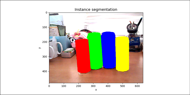
Figure 12.1.1: Four images showing the different segmentation algorithms. Best viewed in color. The original images can be found at https://github.com/PacktPublishing/Advanced-Deep-Learning-with-Keras/tree/master/chapter12-segmentation

2. Semantic segmentation network

From the previous section, we learned that the semantic segmentation network is a pixel-wise classifier. The network block diagram is shown in Figure 12.2.1. However, unlike a simple classifier (for example, the MNIST classifier in Chapter 1, Introducing Advanced Deep Learning with Keras and Chapter 2, Deep Neural Networks), where there is only one classifier generating a one-hot vector as output, in semantic segmentation, we have parallel classifiers running simultaneously. Each one is generating its own one-hot vector prediction. The number of classifiers is equal to the number of pixels in the input image or the product of image width and height. The dimension of each one-hot vector prediction is equal to the number of stuff object categories of interest.

Figure 12.2.1: The semantic segmentation network can be viewed as a pixel-wise classifier. Best viewed in color. The original images can be found at https://github.com/PacktPublishing/Advanced-Deep-Learning-with-Keras/tree/master/chapter12-segmentation

For example, assuming we are interested in four of the categories: 0) Background, 1) Water bottle, 2) Soda can, and 3) Juice can, we can see in Figure 12.2.2 that there are four pixels from each object category.

Each pixel is classified accordingly using a 4-dim one-hot vector. We use color shading to indicate the class category of the pixel. Using this knowledge, we can imagine that a semantic segmentation network predicts image_width x image_height 4-dim one-hot vectors as output, and one 4-dim one-hot vector per pixel:

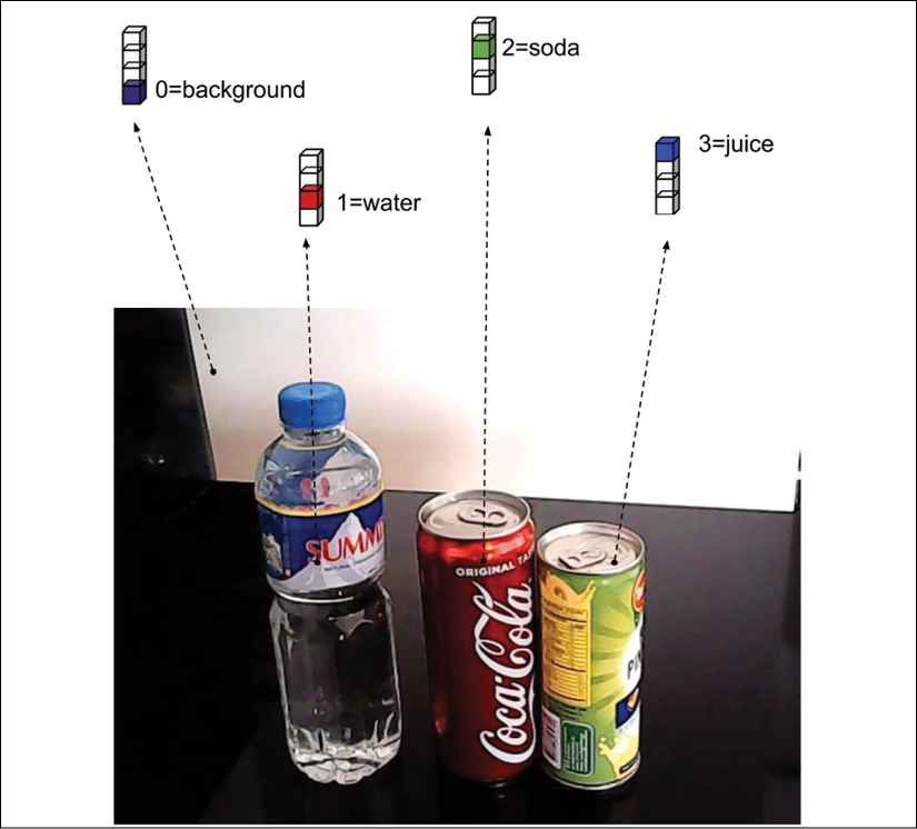
Figure 12.2.2: Four different sample pixels. Using a 4-dim one-hot vector, each pixel is classified according to its category. Best viewed in color. The original images can be found at https://github.com/PacktPublishing/Advanced-Deep-Learning-with-Keras/tree/master/chapter12-segmentation

Having understood the concept of semantic segmentation, we can now introduce a neural network pixel-wise classifier. Our semantic segmentation network architecture is inspired by Fully Convolutional Network (FCN) by Long et al. (2015) [2]. The key idea of FCN is to use multiple scales of feature maps in generating the final prediction.

Our semantic segmentation network is shown in Figure 12.2.3. Its input is an RGB image (for example, 640 x 480 x 3) and it outputs a tensor with similar dimensions except that the last dimension is the number of stuff categories (for example, 640 x 480 x 4 for a 4-stuff category). For visualization purposes, we map the output into RGB by assigning a color to each category:

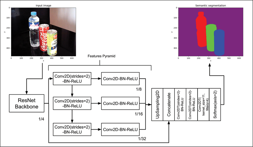
Figure 12.2.3: Network architecture of semantic segmentation. Kernel size is 3 unless indicated. Strides is 1 unless indicated. Best viewed in color. The original images can be found at https://github.com/PacktPublishing/Advanced-Deep-Learning-with-Keras/tree/master/chapter12-segmentation

Similar to SSD that was discussed in Chapter 11, Object Detection, we employ a backbone network as a feature extractor. We use a similar ResNetv2 network in SSD. The ResNet backbone performs max pooling twice to arrive at the first set of feature maps with the dimensions being of the input image. The additional sets of feature maps are generated by using successive Conv2D(strides=2)-BN-ReLU layers, resulting in feature maps with dimensions of the input image.

Our semantic segmentation network architecture is further enhanced by the improvements made by Pyramid Scene Parsing Network (PSPNet) by Zhao et al. (2017) [3]. In PSPNet, each feature map is further processed by another convolutional layer. Furthermore, the first set of feature maps is also used.

Both FCN and PSPNet upsample the features pyramid to arrive at the same size as the first set of feature maps. Afterward, all upsampled features are fused together using a Concatenate layer. The concatenated layers are then processed twice by a transposed convolution with strides equal to 2 to put the original image width and height back. Lastly, a transposed convolution with a kernel size of 1 and filters equal to 4 (in other words, the number of categories) and a Softmax layer are used to generate the pixel-wise categorical prediction.

In the next section, we will discuss the tf.keras implementation of our segmentation network. We can reuse some network blocks in SSD from Chapter 11, Object Detection, to speed up our implementation.

3. Semantic segmentation network in Keras

As shown in Figure 12.2.3, we already have some of the key building blocks of our semantic segmentation network. We can reuse the ResNet model presented in Chapter 2, Deep Neural Networks. We just need to build the features' pyramid and the upsampling and prediction layers.

Borrowing the ResNet model that we developed in Chapter 2, Deep Neural Networks, and which was reused in Chapter 11, Object Detection, we extract a features' pyramid with four levels. Listing 12.3.1 shows features' pyramid extraction from ResNet. conv_layer() is just a helper function to create a Conv2D(strides=2)-BN-ReLU layer.

Listing 12.3.1: resnet.py:

Features' pyramid function:

def features_pyramid(x, n_layers):
    """Generate features pyramid from the output of the 
    last layer of a backbone network (e.g. ResNetv1 or v2)

    Arguments:
        x (tensor): Output feature maps of a backbone network
        n_layers (int): Number of additional pyramid layers

    Return:
        outputs (list): Features pyramid 
    """
    outputs = [x]
    conv = AveragePooling2D(pool_size=2, name='pool1')(x)
    outputs.append(conv)
    prev_conv = conv
    n_filters = 512

    # additional feature map layers
    for i in range(n_layers - 1):
        postfix = "_layer" + str(i+2)
        conv = conv_layer(prev_conv,
                          n_filters,
                          kernel_size=3,
                          strides=2,
                          use_maxpool=False,
                          postfix=postfix)
        outputs.append(conv)
        prev_conv = conv

    return outputs

Listing 12.3.1 is just half of the features' pyramid. The remaining half is the convolution after each set of features. The other half is shown in Listing 12.3.2, together with the upsampling of each level of the pyramid. For example, features with dimensions of of the image size are upsampled by 2 to match their dimensions with the first set of features, which are of the image size. In the same listing, we also build the entire segmentation model, from the backbone network to the features' pyramid, to concatenating upsampled features' pyramids, and finally to further feature extractions, upsampling, and prediction. We use the n-dim (for example, 4-dim) Softmax layer at the output layer to perform pixel-wise classification.

Listing 12.3.2: model.py:

Building the semantic segmentation network:

def build_fcn(input_shape,
              backbone,
              n_classes=4):
    """Helper function to build an FCN model.
        
    Arguments:
        backbone (Model): A backbone network
            such as ResNetv2 or v1
        n_classes (int): Number of object classes
            including background.
    """

    inputs = Input(shape=input_shape)
    features = backbone(inputs)

    main_feature = features[0]
    features = features[1:]
    out_features = [main_feature]
    feature_size = 8
    size = 2
    # other half of the features pyramid
    # including upsampling to restore the
    # feature maps to the dimensions
    # equal to 1/4 the image size
    for feature in features:
        postfix = "fcn_" + str(feature_size)
        feature = conv_layer(feature,
                             filters=256,
                             use_maxpool=False,
                             postfix=postfix)
        postfix = postfix + "_up2d"
        feature = UpSampling2D(size=size,
                               interpolation='bilinear',
                               name=postfix)(feature)
        size = size * 2
        feature_size = feature_size * 2
        out_features.append(feature)

    # concatenate all upsampled features
    x = Concatenate()(out_features)
    # perform 2 additional feature extraction 
    # and upsampling
    x = tconv_layer(x, 256, postfix="up_x2")
    x = tconv_layer(x, 256, postfix="up_x4")
    # generate the pixel-wise classifier
    x = Conv2DTranspose(filters=n_classes,
                        kernel_size=1,
                        strides=1,
                        padding='same',
                        kernel_initializer='he_normal',
                        name="pre_activation")(x)
    x = Softmax(name="segmentation")(x)

    model = Model(inputs, x, name="fcn")

    return model

Given the segmentation network model, we use the Adam optimizer with a learning rate of 1e-3 and a categorical cross-entropy loss function to train the network. Listing 12.3.3 shows the model building and train function calls. The learning rate is halved every 20 epochs after 40 epochs. We monitor the network performance using the AccuracyCallback, similar to the SSD network in Chapter 11, Object Detection. The callback computes the performance using mean IoU (mIoU) metrics similar to the mean IoU for object detection. The weights of the best performing mean IoU are saved on a file. The network is trained for 100 epochs by calling fit_generator().

Listing 12.3.3: fcn-12.3.1.py:

Initialization and training of a semantic segmentation network:

    def build_model(self):
        """Build a backbone network and use it to
            create a semantic segmentation 
            network based on FCN.
        """

        # input shape is (480, 640, 3) by default
        self.input_shape = (self.args.height,
                            self.args.width,
                            self.args.channels)

        # build the backbone network (eg ResNet50)
        # the backbone is used for 1st set of features
        # of the features pyramid
        self.backbone = self.args.backbone(self.input_shape,
                                           n_layers=self.args.layers)

        # using the backbone, build fcn network
        # output layer is a pixel-wise classifier
        self.n_classes =  self.train_generator.n_classes
        self.fcn = build_fcn(self.input_shape,
                             self.backbone,
                             self.n_classes)

    def train(self):
        """Train an FCN"""
        optimizer = Adam(lr=1e-3)
        loss = 'categorical_crossentropy'
        self.fcn.compile(optimizer=optimizer, loss=loss)

        log = "# of classes %d" % self.n_classes
        print_log(log, self.args.verbose)
        log = "Batch size: %d" % self.args.batch_size
        print_log(log, self.args.verbose)

        # prepare callbacks for saving model weights
        # and learning rate scheduler
        # model weights are saved when test iou is highest
        # learning rate decreases by 50% every 20 epochs
        # after 40th epoch
        accuracy = AccuracyCallback(self)
        scheduler = LearningRateScheduler(lr_scheduler)

        callbacks = [accuracy, scheduler]
        # train the fcn network
        self.fcn.fit_generator(generator=self.train_generator,
                               use_multiprocessing=True,
                               callbacks=callbacks,
                               epochs=self.args.epochs,
                               workers=self.args.workers)

The multithreaded data generator class, DataGenerator, is similar to what was used in Chapter 11, Object Detection. As shown in Listing 12.3.4, the __data_generation (self, keys) signature method was modified to generate a pair of image tensors and its corresponding pixel-wise ground truth labels or segmentation mask. In the next section, we will discuss how to generate ground truth labels.

Listing 12.3.4: data_generator.py:

Data generation method of the DataGenerator class for semantic segmentation:

    def __data_generation(self, keys):
        """Generate train data: images and 
        segmentation ground truth labels 

        Arguments:
            keys (array): Randomly sampled keys
                (key is image filename)

        Returns:
            x (tensor): Batch of images
            y (tensor): Batch of pixel-wise categories
        """
        # a batch of images
        x = []
        # and their corresponding segmentation masks
        y = []

        for i, key in enumerate(keys):
            # images are assumed to be stored 
            # in self.args.data_path
            # key is the image filename 
            image_path = os.path.join(self.args.data_path, key)
            image = skimage.img_as_float(imread(image_path))
            # append image to the list
            x.append(image)
            # and its corresponding label (segmentation mask)
            labels = self.dictionary[key]
            y.append(labels)

        return np.array(x), np.array(y)

The semantic segmentation network is now complete. Using tf.keras, we have discussed its architecture implementation, initialization, and training.

Before we can run the training procedure, we need the training and test datasets with ground truth labels. In the next section, we will discuss the semantic segmentation dataset that we will use in this chapter.

4. Example dataset

We can use the dataset that we used in Chapter 11, Object Detection. Recall that we used a small dataset comprising 1,000 640 x 480 RGB train images and 50 640 x 480 RGB test images collected using an inexpensive USB camera (A4TECH PK-635G). However, instead of labeling using bounding boxes and categories, we traced the edges of each object category using a polygon shape. We used the same dataset annotator called VGG Image Annotator (VIA) [4] to manually trace the edges and assign the following labels: 1) Water bottle, 2) Soda can, and 3) Juice can.

Figure 12.4.1 shows a sample UI of the labeling process.

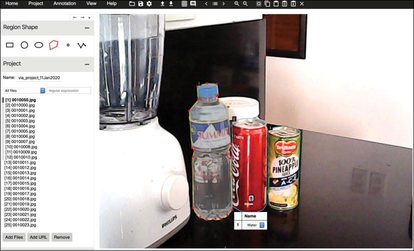
Figure 12.4.1: Dataset labeling process for semantic segmentation using the VGG Image Annotator (VIA)

The VIA labeling software saves the annotation on a JSON file. For the training and test datasets, these are:

segmentation_train.json
segmentation_test.json

The polygon region stored on the JSON files could not be used as it is. Each region has to be converted into a segmentation mask, which is a tensor with the dimensions image_width x image_height x pixel – wise_category. In this dataset, the dimensions of the segmentation mask are 640 x 480 x 4. The category 0 is for background, and the rest are 1) for Water bottle, 2) for Soda can, and 3) for Juice can. In the utils folder, we created a tool, generate_gt_segmentation.py, to convert the JSON file into segmentation masks. For convenience, the ground truth data for training and testing is stored inside the compressed dataset, which we downloaded from https://bit.ly/adl2-ssd in the previous chapter:

segmentation_train.npy
segmentation_test.npy

Each file contains a dictionary of ground truth data in the format image filename: segmentation mask, which is loaded during training and validation. Figure 12.4.2 shows an example of the segmentation mask of the image in Figure 12.4.1, visualized using colored pixels.

Figure 12.4.2: Visualization of the segmentation mask for the annotation done in Figure 12.4.1

We are now ready to train and validate the semantic segmentation network. In the next section, we will show the results of the semantic segmentation on the dataset that we annotated in this section.

5. Semantic segmentation validation

To train the semantic segmentation network, run the following command:

python3 fcn-12.3.1.py --train

At every epoch, the validation is also executed to determine the best performing parameters. For semantic segmentation, two metrics can be used. The first is mean IoU. This is similar to the mean IoU in object detection in the previous chapter. The difference is that the IoU is computed between the ground truth segmentation mask and the predicted segmentation mask for each stuff category. This includes the background. The mean IoU is simply the average of all IoUs for the test dataset.

Figure 12.5.1 shows the performance of our semantic segmentation network using mIoU at every epoch. The maximum mIoU is 0.91. This is relatively high. However, our dataset only has four object categories:

Figure 12.5.1: Semantic segmentation performance during training using mIoU for the test dataset

The second metric is average pixel accuracy. This is similar to how the accuracy is computed on a classifier prediction. The difference is that, instead of having one prediction, the segmentation network has a number of predictions equal to the number of pixels in the image. For each test input image, an average pixel accuracy is computed. Then, the mean for all the test images is computed.

Figure 12.5.2 shows the performance of our semantic segmentation network using average pixel accuracy at every epoch. The maximum average pixel accuracy is 97.9%. We can see the correlation between average pixel accuracy and mIoU:

Figure 12.5.2: Semantic segmentation performance during training using average pixel accuracy for the test dataset

Figure 12.5.3 shows a sample of the input image, the ground truth semantic segmentation mask, and the predicted semantic segmentation mask:

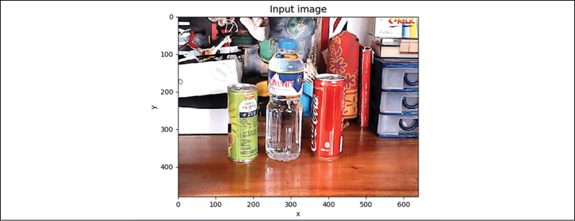
Figure 12.5.3: Sample input, ground truth, and prediction for semantic segmentation. We assigned the color black for the background class instead of purple, as was used earlier

Overall, our semantic segmentation network that is based on FCN and improved by ideas from PSPNet is performing relatively well. Our semantic segmentation network is by no means optimized. The number of filters in the features' pyramid can be reduced to minimize the number of parameters, which is about 11.1 million. It is also interesting to explore increasing the number of levels in the features' pyramid. The reader may run validation by executing:

python3 fcn-12.3.1.py --evaluate 
--restore-weights=ResNet56v2-3layer-drinks-best-iou.h5

In the next chapter, we will introduce unsupervised learning algorithms. There has been a strong motivation to develop unsupervised learning techniques considering the costly and time-consuming labeling needed in supervised learning. For example, in the semantic segmentation dataset in this chapter, it took one person about 4 days of manual labeling. Deep learning will not advance if it requires human labeling all the time.

6. Conclusion

In this chapter, the concept of segmentation was discussed. We learned that there are different categories of segmentation. Each has its own target application. This chapter focused on the network design, implementation, and validation of semantic segmentation.

Our semantic segmentation network was inspired by FCN, which has been the basis of many modern-day, state-of-the-art segmentation algorithms, such as Mask-R-CNN [5]. Our network was further enhanced by ideas from PSPNet, which won first place in the ImageNet 2016 parsing challenge.

Using the VIA labeling tool, a new dataset label for semantic segmentation was generated using the same set of images employed in Chapter 11, Object Detection. The segmentation mask labels all pixels belonging to the same object class.

Our semantic segmentation network was trained and validated using mean IoU and average pixel accuracy metrics. The performance on the test dataset shows that it can effectively classify pixels in our test images.

As mentioned in the last section of this chapter, the field of deep learning is realizing the limits of supervised learning due to the costs and time involved. The next chapter focuses on unsupervised learning. It takes advantage of the concept of mutual information that is used in information theory in the field of communications.

7. References

1. Kirillov, Alexander, et al.: Panoptic Segmentation. Proceedings of the IEEE conference on computer vision and pattern recognition. 2019.
2. Long, Jonathan, Evan Shelhamer, and Trevor Darrell: Fully Convolutional Networks for Semantic Segmentation. Proceedings of the IEEE conference on computer vision and pattern recognition. 2015.
3. Zhao, Hengshuang, et al.: Pyramid Scene Parsing Network. Proceedings of the IEEE conference on computer vision and pattern recognition. 2017.
4. Dutta, et al.: VGG Image Annotator http://www.robots.ox.ac.uk/~vgg/software/via/

5. He Kaiming, et al.: Mask R-CNN. Proceedings of the IEEE international conference on computer vision. 2017.