1
Introducing Advanced Deep Learning with Keras
In this first chapter, we will introduce three deep learning artificial neural networks that we will be using throughout the book. These networks are MLP, CNN, and RNN (defined and described in Section 2), which are the building blocks of selected advanced deep learning topics covered in this book, such as autoregressive networks (autoencoder, GAN, and VAE), deep reinforcement learning, object detection and segmentation, and unsupervised learning using mutual information.
Together, we'll discuss how to implement MLP, CNN, and RNN based models using the Keras library in this chapter. More specifically, we will use the TensorFlow Keras library called tf.keras. We'll start by looking at why tf.keras is an excellent choice as a tool for us. Next, we'll dig into the implementation details within the three deep learning networks.
This chapter will:
- Establish why the
tf.keraslibrary is a great choice to use for advanced deep learning - Introduce MLP, CNN, and RNN – the core building blocks of advanced deep learning models, which we'll be using throughout this book
- Provide examples of how to implement MLP, CNN, and RNN based models using
tf.keras - Along the way, start to introduce important deep learning concepts, including optimization, regularization, and loss function
By the end of this chapter, we'll have the fundamental deep learning networks implemented using tf.keras. In the next chapter, we'll get into the advanced deep learning topics that build on these foundations. Let's begin this chapter by discussing Keras and its capabilities as a deep learning library.
1. Why is Keras the perfect deep learning library?
Keras [1] is a popular deep learning library with over 370,000 developers using it at the time of writing – a number that is increasing by about 35% every year. Over 800 contributors actively maintain it. Some of the examples we'll use in this book have been contributed to the official Keras GitHub repository.
Google's TensorFlow, a popular open source deep learning library, uses Keras as a high-level API for its library. It is commonly called tf.keras. In this book, we will use the word Keras and tf.keras interchangeably.
tf.keras is a popular choice as a deep learning library since it is highly integrated into TensorFlow, which is known in production deployments for its reliability. TensorFlow also offers various tools for production deployment and maintenance, debugging and visualization, and running models on embedded devices and browsers. In the technology industry, Keras is used by Google, Netflix, Uber, and NVIDIA.
We have chosen tf.keras as our tool of choice to work with in this book because it is a library dedicated to accelerating the implementation of deep learning models. This makes Keras ideal for when we want to be practical and hands-on, such as when we're exploring the advanced deep learning concepts in this book. Because Keras is designed to accelerate the development, training, and validation of deep learning models, it is essential to learn the key concepts in this field before someone can maximize the use of the library.
All of the examples in this book can be found on GitHub at the following link: https://github.com/PacktPublishing/Advanced-Deep-Learning-with-Keras.
In the tf.keras library, layers are connected to one another like pieces of Lego, resulting in a model that is clean and easy to understand. Model training is straightforward, requiring only data, a number of epochs of training, and metrics to monitor.
The end result is that most deep learning models can be implemented with significantly fewer lines of code compared to other deep learning libraries such as PyTorch. By using Keras, we'll boost productivity by saving time in code implementation, which can instead be spent on more critical tasks such as formulating better deep learning algorithms.
Likewise, Keras is ideal for the rapid implementation of deep learning models, like the ones that we will be using in this book. Typical models can be built in just a few lines of code using the Sequential model API. However, do not be misled by its simplicity.
Keras can also build more advanced and complex models using its functional API and Model and Layer classes for dynamic graphs, which can be customized to satisfy unique requirements. The functional API supports building graph-like models, layer reuse, and creating models that behave like Python functions. Meanwhile, the Model and Layer classes provide a framework for implementing uncommon or experimental deep learning models and layers.
Installing Keras and TensorFlow
Keras is not an independent deep learning library. As you can see in Figure 1.1.1, it is built on top of another deep learning library or backend. This could be Google's TensorFlow, MILA's Theano, Microsoft's CNTK, or Apache MXNet. However, unlike the previous edition of this book, we will use Keras as provided by TensorFlow 2.0 (tf2 or simply tf), which is better known as tf.keras, to take advantage of the useful tools offered by tf2. tf.keras is also considered the de facto frontend of TensorFlow, which has exhibited its proven reliability in the production environment. Furthermore, Keras' support for backends other than TensorFlow will no longer be available in the near future.
Migration from Keras to tf.keras is generally as straightforward as changing:
from keras... import ...
to
from tensorflow.keras... import ...
In this book, the code examples are all written in Python 3 as support for Python 2 ends in the year 2020.
On hardware, Keras runs on a CPU, GPU, and Google's TPU. In this book, we'll test on a CPU and NVIDIA GPUs (specifically, the GTX 1060, GTX 1080Ti, RTX 2080Ti, V100, and Quadro RTX 8000 models):

Figure 1.1.1: Keras is a high-level library that sits on top of other deep learning frameworks. Keras is supported on CPU, GPU, and TPU.
Before proceeding with the rest of the book, we need to ensure that tf2 is correctly installed. There are multiple ways to perform the installation; one example is by installing tf2 using pip3:
$ sudo pip3 install tensorflow
If we have a supported NVIDIA GPU, with properly installed drivers, and both NVIDIA CUDA toolkit and the cuDNN Deep Neural Network library, it is highly recommended that you install the GPU-enabled version since it can accelerate both training and predictions:
$ sudo pip3 install tensorflow-gpu
There is no need to install Keras as it is already a package in tf2. If you are uncomfortable installing libraries system-wide, it is highly recommended to use an environment such as Anaconda (https://www.anaconda.com/distribution/). Other than having an isolated environment, the Anaconda distribution installs commonly used third-party packages for data sciences that are indispensable for deep learning.
The examples presented in this book will require additional packages, such as pydot, pydot_ng, vizgraph, python3-tk, and matplotlib. We'll need to install these packages before proceeding beyond this chapter.
The following should not generate any errors if tf2 is installed along with its dependencies:
$ python3
>>> import tensorflow as tf
>>> print(tf.__version__)
2.0.0
>>> from tensorflow.keras import backend as K
>>> print(K.epsilon())
1e-07
This book does not cover the complete Keras API. We'll only be covering the materials needed to explain selected advanced deep learning topics in this book. For further information, we can consult the official Keras documentation, which can be found at https://keras.io or https://www.tensorflow.org/guide/keras/overview.
In the succeeding sections, the details of MLP, CNN, and RNN will be discussed. These networks will be used to build a simple classifier using tf.keras.
2. MLP, CNN, and RNN
We've already mentioned that we'll be using three deep learning networks, they are:
- MLP: Multilayer Perceptron
- CNN: Convolutional Neural Network
- RNN: Recurrent Neural Network
These are the three networks that we will be using throughout this book. Later on, you'll find that they are often combined together in order to take advantage of the strength of each network.
In this chapter, we'll discuss these building blocks one by one in more detail. In the following sections, MLP is covered alongside other important topics such as loss functions, optimizers, and regularizers. Following this, we'll cover both CNNs and RNNs.
The differences between MLP, CNN, and RNN
An MLP is a fully connected (FC) network. You'll often find it referred to as either deep feed-forward network or feed-forward neural network in some literature. In this book, we will use the term MLP. Understanding this network in terms of known target applications will help us to get insights about the underlying reasons for the design of the advanced deep learning models.
MLPs are common in simple logistic and linear regression problems. However, MLPs are not optimal for processing sequential and multi-dimensional data patterns. By design, an MLP struggles to remember patterns in sequential data and requires a substantial number of parameters to process multi-dimensional data.
For sequential data input, RNNs are popular because the internal design allows the network to discover dependency in the history of the data, which is useful for prediction. For multi-dimensional data like images and videos, CNNs excel in extracting feature maps for classification, segmentation, generation, and other downstream tasks. In some cases, a CNN in the form of a 1D convolution is also used for networks with sequential input data. However, in most deep learning models, MLP and CNN or RNN are combined to make the most out of each network.
MLP, CNN, and RNN do not complete the whole picture of deep networks. There is a need to identify an objective or loss function, an optimizer, and a regularizer. The goal is to reduce the loss function value during training, since such a reduction is a good indicator that a model is learning.
To minimize this value, the model employs an optimizer. This is an algorithm that determines how weights and biases should be adjusted at each training step. A trained model must work not only on the training data but also on data outside of the training environment. The role of the regularizer is to ensure that the trained model generalizes to new data.
Now, let's get into the three networks – we'll begin by talking about the MLP network.
3. Multilayer Perceptron (MLP)
The first of the three networks we will be looking at is the MLP network. Let's suppose that the objective is to create a neural network for identifying numbers based on handwritten digits. For example, when the input to the network is an image of a handwritten number 8, the corresponding prediction must also be the digit 8. This is a classic job of classifier networks that can be trained using logistic regression. To both train and validate a classifier network, there must be a sufficiently large dataset of handwritten digits. The Modified National Institute of Standards and Technology dataset, or MNIST [2] for short, is often considered as the Hello World! of deep learning datasets. It is a suitable dataset for handwritten digit classification.
Before we discuss the MLP classifier model, it's essential that we understand the MNIST dataset. A large number of examples in this book use the MNIST dataset. MNIST is used to explain and validate many deep learning theories because the 70,000 samples it contains are small, yet sufficiently rich in information:

Figure 1.3.1: Example images from the MNIST dataset. Each grayscale image is 28 × 28-pixels.
In the following section, we'll briefly introduce MNIST.
The MNIST dataset
MNIST is a collection of handwritten digits ranging from 0 to 9. It has a training set of 60,000 images, and 10,000 test images that are classified into corresponding categories or labels. In some literature, the term target or ground truth is also used to refer to the label.
In the preceding figure, sample images of the MNIST digits, each being sized at 28 x 28 - pixel, in grayscale, can be seen. To use the MNIST dataset in Keras, an API is provided to download and extract images and labels automatically. Listing 1.3.1 demonstrates how to load the MNIST dataset in just one line, allowing us to both count the train and test labels and then plot 25 random digit images.
Listing 1.3.1: mnist-sampler-1.3.1.py
import numpy as np
from tensorflow.keras.datasets import mnist
import matplotlib.pyplot as plt
# load dataset
(x_train, y_train), (x_test, y_test) = mnist.load_data()
# count the number of unique train labels
unique, counts = np.unique(y_train, return_counts=True)
print("Train labels: ", dict(zip(unique, counts)))
# count the number of unique test labels
unique, counts = np.unique(y_test, return_counts=True)
print("Test labels: ", dict(zip(unique, counts)))
# sample 25 mnist digits from train dataset
indexes = np.random.randint(0, x_train.shape[0], size=25)
images = x_train[indexes]
labels = y_train[indexes]
# plot the 25 mnist digits
plt.figure(figsize=(5,5))
for i in range(len(indexes)):
    plt.subplot(5, 5, i + 1)
    image = images[i]
    plt.imshow(image, cmap='gray')
    plt.axis('off')
plt.savefig("mnist-samples.png")
plt.show()
plt.close('all')
The mnist.load_data() method is convenient since there is no need to load all 70,000 images and labels individually and store them in arrays. Execute the following:
python3 mnist-sampler-1.3.1.py
On the command line, the code example prints the distribution of labels in the train and test datasets:
Train labels:{0: 5923, 1: 6742, 2: 5958, 3: 6131, 4: 5842, 5: 5421, 6: 5918, 7: 6265, 8: 5851, 9: 5949}
Test labels:{0: 980, 1: 1135, 2: 1032, 3: 1010, 4: 982, 5: 892, 6: 958, 7: 1028, 8: 974, 9: 1009}
Afterward, the code will plot 25 random digits, as shown in previously in Figure 1.3.1.
Before discussing the MLP classifier model, it is essential to keep in mind that while the MNIST data consists of two dimensional tensors, it should be reshaped depending on the type of input layer. The following Figure 1.3.2 shows how a 3 × 3 grayscale image is reshaped for MLP, CNN, and RNN input layers:

Figure 1.3.2: An input image similar to the MNIST data is reshaped depending on the type of input layer. For simplicity, the reshaping of a 3 × 3 grayscale image is shown.
In the following sections, an MLP classifier model for MNIST will be introduced. We will demonstrate how to efficiently build, train, and validate the model using tf.keras.
The MNIST digit classifier model
The proposed MLP model shown in Figure 1.3.3 can be used for MNIST digit classification. When the units or perceptrons are exposed, the MLP model is a fully connected network, as shown in Figure 1.3.4. We will also show how the output of the perceptron is computed from inputs as a function of weights, wi, and bias, bn, for the n-th unit. The corresponding tf.keras implementation is illustrated in Listing 1.3.2:

Figure 1.3.3: The MLP MNIST digit classifier model

Figure 1.3.4: The MLP MNIST digit classifier in Figure 1.3.3 is made of fully connected layers. For simplicity, the activation and dropout layers are not shown. One unit or perceptron is also shown in detail.
Listing 1.3.2: mlp-mnist-1.3.2.py
import numpy as np
from tensorflow.keras.models import Sequential
from tensorflow.keras.layers import Dense, Activation, Dropout
from tensorflow.keras.utils import to_categorical, plot_model
from tensorflow.keras.datasets import mnist
# load mnist dataset
(x_train, y_train), (x_test, y_test) = mnist.load_data()
# compute the number of labels
num_labels = len(np.unique(y_train))
# convert to one-hot vector
y_train = to_categorical(y_train)
y_test = to_categorical(y_test)

# image dimensions (assumed square)
image_size = x_train.shape[1]
input_size = image_size * image_size
# resize and normalize
x_train = np.reshape(x_train, [-1, input_size])
x_train = x_train.astype('float32') / 255
x_test = np.reshape(x_test, [-1, input_size])
x_test = x_test.astype('float32') / 255
# network parameters
batch_size = 128
hidden_units = 256
dropout = 0.45
# model is a 3-layer MLP with ReLU and dropout after each layer
model = Sequential()
model.add(Dense(hidden_units, input_dim=input_size))
model.add(Activation('relu'))
model.add(Dropout(dropout))
model.add(Dense(hidden_units))
model.add(Activation('relu'))
model.add(Dropout(dropout))
model.add(Dense(num_labels))
# this is the output for one-hot vector
model.add(Activation('softmax'))
model.summary()
plot_model(model, to_file='mlp-mnist.png', show_shapes=True)
# loss function for one-hot vector
# use of adam optimizer
# accuracy is good metric for classification tasks
model.compile(loss='categorical_crossentropy',
              optimizer='adam',
              metrics=['accuracy'])
# train the network
model.fit(x_train, y_train, epochs=20, batch_size=batch_size)
# validate the model on test dataset to determine generalization
_, acc = model.evaluate(x_test,
                        y_test,
                        batch_size=batch_size,
                        verbose=0)
print("
Test accuracy: %.1f%%" % (100.0 * acc))
Before discussing the model implementation, the data must be in the correct shape and format. After loading the MNIST dataset, the number of labels is computed as:
# compute the number of labels
num_labels = len(np.unique(y_train))
Hardcoding num_labels = 10 is also an option. But, it's always a good practice to let the computer do its job. The code assumes that y_train has labels 0 to 9.
At this point, the labels are in digit format, that is, from 0 to 9. This sparse scalar representation of labels is not suitable for the neural network prediction layer that outputs probabilities per class. A more suitable format is called a one-hot vector, a 10-dimensional vector with all elements 0, except for the index of the digit class. For example, if the label is 2, the equivalent one-hot vector is [0,0,1,0,0,0,0,0,0,0]. The first label has index 0.
The following lines convert each label into a one-hot vector:
# convert to one-hot vector
y_train = to_categorical(y_train)
y_test = to_categorical(y_test)
In deep learning, data are stored in tensors. The term tensor applies to a scalar (0D tensor), vector (1D tensor), matrix (two dimensional tensor), and multi-dimensional tensor.
From this point, the term tensor is used unless scalar, vector, or matrix makes the explanation clearer.
The rest of the code as shown below computes the image dimensions, the input_size value of the first dense layer, and scales each pixel value from 0 to 255 to range from 0.0 to 1.0. Although raw pixel values can be used directly, it is better to normalize the input data so as to avoid large gradient values that could make training difficult. The output of the network is also normalized. After training, there is an option to put everything back to the integer pixel values by multiplying the output tensor by 255.
The proposed model is based on MLP layers. Therefore, the input is expected to be a 1D tensor. As such, x_train and x_test are reshaped to [60,000, 28 * 28] and [10,000, 28 * 28], respectively. In NumPy, a size of -1 means to let the library compute the correct dimension. In the case of x_train, this is 60,000.
# image dimensions (assumed square) 400
image_size = x_train.shape[1]
input_size = image_size * image_size
# resize and normalize
x_train = np.reshape(x_train, [-1, input_size])
x_train = x_train.astype('float32') / 255
x_test = np.reshape(x_test, [-1, input_size])
x_test = x_test.astype('float32') / 255
After preparing the dataset, the following focuses on building the MLP classifier model using the Sequential API of Keras.
Building a model using MLP and Keras
After the data preparation, building the model is next. The proposed model is made of three MLP layers. In Keras, an MLP layer is referred to as dense, which stands for the densely connected layer. Both the first and second MLP layers are identical in nature with 256 units each, followed by the Rectified Linear Unit (ReLU) activation and dropout. 256 units are chosen since 128, 512, and 1,024 units have lower performance metrics. At 128 units, the network converges quickly but has a lower test accuracy. The additional number of units for 512 or 1,024 does not significantly increase the test accuracy.
The number of units is a hyperparameter. It controls the capacity of the network. The capacity is a measure of the complexity of the function that the network can approximate. For example, for polynomials, the degree is the hyperparameter. As the degree increases, the capacity of the function also increases.
As shown in the following lines of code, the classifier model is implemented using the Sequential API of Keras. This is sufficient if the model requires one input and one output as processed by a sequence of layers. For simplicity, we'll use this for now; however, in Chapter 2, Deep Neural Networks, the Functional API of Keras will be introduced to implement advanced deep learning models that require more complex structures such as multiple inputs and outputs.
# model is a 3-layer MLP with ReLU and dropout after each layer model = Sequential()
model.add(Dense(hidden_units, input_dim=input_size))
model.add(Activation('relu'))
model.add(Dropout(dropout))
model.add(Dense(hidden_units))
model.add(Activation('relu'))
model.add(Dropout(dropout))
model.add(Dense(num_labels))
# this is the output for one-hot vector model.add(Activation('softmax'))
Since a Dense layer is a linear operation, a sequence of Dense layers can only approximate a linear function. The problem is that the MNIST digit classification is inherently a non-linear process. Inserting a relu activation between the Dense layers will enable an MLP network to model non-linear mappings. relu or ReLU is a simple non-linear function. It's very much like a filter that allows positive inputs to pass through unchanged while clamping everything else to zero. Mathematically, relu is expressed in the following equation and is plotted in Figure 1.3.5:


Figure 1.3.5: Plot of the ReLU function. The ReLU function introduces non-linearity in neural networks.
There are other non-linear functions that can be used, such as elu, selu, softplus, sigmoid, and tanh. However, relu is the most commonly used function and is computationally efficient due to its simplicity. The sigmoid and tanh functions are used as activation functions in the output layer and will be described later. Table 1.3.1 shows the equation for each of these activation functions:
|
|
relu(x) = max(0, x) |
1.3.1 |
|
|
softplus(x) = log(1 + ex) |
1.3.2 |
|
|
where a ≥ 0 and is a tunable hyperparameter |
1.3.3 |
|
|
selu(x) = k × elu(x, a) where k = 1.0507009873554804934193349852946 and a = 1.6732632423543772848170429916717 |
1.3.4 |
|
|
|
1.3.5 |
|
|
|
1.3.6 |


Table 1.3.1: Definition of common non-linear activation functions
Although we have completed the key layers of the MLP classifier model, we have not addressed the issue of generalization or the ability of the model to perform beyond the train dataset. To address this issue, we will introduce regularization in the next section.
Regularization
A neural network has the tendency to memorize its training data, especially if it contains more than enough capacity. In such cases, the network fails catastrophically when subjected to the test data. This is the classic case of the network failing to generalize. To avoid this tendency, the model uses a regularizing layer or function. A common regularizing layer is Dropout.
The idea of dropout is simple. Given a dropout rate (here, it is set to dropout = 0.45), the Dropout layer randomly removes that fraction of units from participating in the next layer. For example, if the first layer has 256 units, after dropout = 0.45 is applied, only (1 - 0.45) * 256 units = 140 units from layer 1 participate in layer 2.
The Dropout layer makes neural networks robust to unforeseen input data because the network is trained to predict correctly, even if some units are missing. It's worth noting that dropout is not used in the output layer and it is only active during training. Moreover, dropout is not present during predictions.
There are regularizers that can be used other than dropouts such as l1 or l2. In Keras, the bias, weight, and activation outputs can be regularized per layer. l1 and l2 favor smaller parameter values by adding a penalty function. Both l1 and l2 enforce the penalty using a fraction of the sum of the absolute (l1) or square (l2) of parameter values. In other words, the penalty function forces the optimizer to find parameter values that are small. Neural networks with small parameter values are more insensitive to the presence of noise from within the input data.
As an example, an l2-weight regularizer with fraction=0.001 can be implemented as:
from tensorflow.keras.regularizers import l2
model.add(Dense(hidden_units,
                kernel_regularizer=l2(0.001),
                input_dim=input_size))
No additional layer is added if an l1 or l2 regularization is used. The regularization is imposed in the Dense layer internally. For the proposed model, dropout still has a better performance than l2.
We are almost complete with our model. The next section focuses on the output layer and loss function.
Output activation and loss function
The output layer has 10 units followed by a softmax activation layer. The 10 units correspond to the 10 possible labels, classes, or categories. The softmax activation can be expressed mathematically, as shown in the following equation:
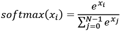 (Equation 1.3.7)
The equation is applied on all N = 10 outputs, xi for i = 0, 1 … 9 for the final prediction. The idea of softmax is surprisingly simple. It squashes the outputs into probabilities by normalizing the prediction. Here, each predicted output is a probability that the index is the correct label of the given input image. The sum of all the probabilities for all outputs is 1.0. For example, when the softmax layer generates a prediction, it will be a 10-dim 1D tensor that may look like the following output:
|
|
|
|
|
|
|
|
The prediction output tensor suggests that the input image is going to be 7 given that its index has the highest probability. The numpy.argmax() method can be used to determine the index of the element with the highest value.
There are other choices of output activation layer, such as linear, sigmoid, or tanh. The linear activation is an identity function. It copies its input to its output. The sigmoid function is more specifically known as a logistic sigmoid. This will be used if the elements of the prediction tensor will be independently mapped between 0.0 and 1.0. The summation of all the elements of the predicted tensor is not constrained to 1.0 unlike in softmax. For example, sigmoid is used as the last layer in sentiment prediction (from 0.0 to 1.0, 0.0 being bad, and 1.0 being good) or in image generation (0.0 is mapped to pixel level 0 and 1.0 is mapped to pixel 255).
The tanh function maps its input in the range -1.0 to 1.0. This is important if the output can swing in both positive and negative values. The tanh function is more popularly used in the internal layer of recurrent neural networks but has also been used as an output layer activation. If tanh is used to replace sigmoid in the output activation, the data used must be scaled appropriately. For example, instead of scaling each grayscale pixel in the range [0.0 1.0] using ![]() , it is assigned in the range [-1.0 to 1.0] using
, it is assigned in the range [-1.0 to 1.0] using  .
.
The following graph in Figure 1.3.6 shows the sigmoid and tanh functions. Mathematically, sigmoid can be expressed in the following equation:
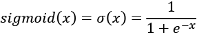 (Equation 1.3.5)
Figure 1.3.6: Plots of sigmoid and tanh
How far the predicted tensor is from the one-hot ground truth vector is called loss. One type of loss function is mean_squared_error (MSE), or the average of the squares of the differences between the target or label and the prediction. In the current example, we are using categorical_crossentropy. It's the negative of the sum of the product of the target or label and the logarithm of the prediction per category. There are other loss functions that are available in Keras, such as mean_absolute_error and binary_crossentropy. Table 1.3.2 summarizes the common loss functions.
| Loss Function | Equation |
|
|
|
|
|
|
|
|
|
|
|
|


Table 1.3.2: Summary of common loss functions. Categories refers to the number of classes (for example: 10 for MNIST) in both the label and the prediction. Loss equations shown are for one output only. The mean loss value is the average for the entire batch.
The choice of the loss function is not arbitrary but should be a criterion that the model is learning. For classification by category, either categorical_crossentropy or mean_squared_error is a good choice after the softmax activation layer. The binary_crossentropy loss function is normally used after the sigmoid activation layer, while mean_squared_error is an option for the tanh output.
In the next section, we will discuss optimization algorithms to minimize the loss functions that we discussed here.
Optimization
With optimization, the objective is to minimize the loss function. The idea is that if the loss is reduced to an acceptable level, the model has indirectly learned the function that maps inputs to outputs. Performance metrics are used to determine if a model has learned the underlying data distribution. The default metric in Keras is loss. During training, validation, and testing, other metrics such as accuracy can also be included. Accuracy is the percentage, or fraction, of correct predictions based on ground truth. In deep learning, there are many other performance metrics. However, it depends on the target application of the model. In literature, the performance metrics of the trained model on the test dataset is reported for comparison with other deep learning models.
In Keras, there are several choices for optimizers. The most commonly used optimizers are stochastic gradient descent (SGD), Adaptive Moments (Adam), and Root Mean Squared Propagation (RMSprop). Each optimizer features tunable parameters like learning rate, momentum, and decay. Adam and RMSprop are variations of SGD with adaptive learning rates. In the proposed classifier network, Adam is used since it has the highest test accuracy.
SGD is considered the most fundamental optimizer. It's a simpler version of the gradient descent in calculus. In gradient descent (GD), tracing the curve of a function downhill finds the minimum value, much like walking downhill in a valley until the bottom is reached.
The GD algorithm is illustrated in Figure 1.3.7. Let's suppose x is the parameter (for example, weight) being tuned to find the minimum value of y (for example, the loss function). Starting at an arbitrary point of x= -0.5. the gradient 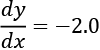 . The GD algorithm imposes that x is then updated to
 ![]() . The new value of x is equal to the old value, plus the opposite of the gradient scaled by
. The new value of x is equal to the old value, plus the opposite of the gradient scaled by ![]() . The small number
. The small number ![]() refers to the learning rate. If
refers to the learning rate. If ![]() = 0.01 then the new value of x = -0.48. GD is performed iteratively. At each step, y will get closer to its minimum value. At x = 0.5,
= 0.01 then the new value of x = -0.48. GD is performed iteratively. At each step, y will get closer to its minimum value. At x = 0.5, ![]() . GD has found the absolute minimum value of y = -1.25. The gradient recommends no further change in x.
. GD has found the absolute minimum value of y = -1.25. The gradient recommends no further change in x.
The choice of learning rate is crucial. A large value of ![]() may not find the minimum value since the search will just swing back and forth around the minimum value. On one hand, a large value of
may not find the minimum value since the search will just swing back and forth around the minimum value. On one hand, a large value of ![]() may take a significant number of iterations before the minimum is found. In the case of multiple minima, the search might get stuck in a local minimum.
may take a significant number of iterations before the minimum is found. In the case of multiple minima, the search might get stuck in a local minimum.

Figure 1.3.7: GD is similar to walking downhill on the function curve until the lowest point is reached. In this plot, the global minimum is at x = 0.5.
An example of multiple minima can be seen in Figure 1.3.8. If for some reason the search started at the left side of the plot and the learning rate is very small, there is a high probability that GD will find x = -1.51 as the minimum value of y. GD will not find the global minimum at x = 1.66. A sufficiently valued learning rate will enable the GD to overcome the hill at x = 0.0.
In deep learning practices, it is normally recommended to start with a bigger learning rate (for example, 0.1 to 0.001) and gradually decrease this as the loss gets closer to the minimum.
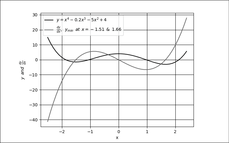
Figure 1.3.8: Plot of a function with 2 minima, x = -1.51 and x = 1.66. Also shown is the derivative of the function.
GD is not typically used in deep neural networks since it is common to encounter millions of parameters to train. It is computationally inefficient to perform a full GD. Instead, SGD is used. In SGD, a mini batch of samples is chosen to compute an approximate value of the descent. The parameters (for example, weights and biases) are adjusted by the following equation:
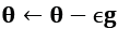
In this equation, ![]() and
and ![]() are the parameters and gradient tensor of the loss function, respectively. The g is computed from partial derivatives of the loss function. The mini-batch size is recommended to be a power of 2 for GPU optimization purposes. In the proposed network,
are the parameters and gradient tensor of the loss function, respectively. The g is computed from partial derivatives of the loss function. The mini-batch size is recommended to be a power of 2 for GPU optimization purposes. In the proposed network, batch_size = 128.
Equation 1.3.8 computes the last layer parameter updates. So, how do we adjust the parameters of the preceding layers? In this case, the chain rule of differentiation is applied to propagate the derivatives to the lower layers and compute the gradients accordingly. This algorithm is known as backpropagation in deep learning. The details of backpropagation are beyond the scope of this book. However, a good online reference can be found at http://neuralnetworksanddeeplearning.com.
Since optimization is based on differentiation, it follows that an important criterion of the loss function is that it must be smooth or differentiable. This is an important constraint to keep in mind when introducing a new loss function.
Given the training dataset, the choice of the loss function, the optimizer, and the regularizer, the model can now be trained by calling the fit() function:
# loss function for one-hot vector
# use of adam optimizer
# accuracy is a good metric for classification tasks model.compile(loss='categorical_crossentropy',
optimizer='adam', metrics=['accuracy'])
# train the network
model.fit(x_train, y_train, epochs=20, batch_size=batch_size)
This is another helpful feature of Keras. By just supplying both the x and y data, the number of epochs to train, and the batch size, fit() does the rest. In other deep learning frameworks, this translates to multiple tasks such as preparing the input and output data in the proper format, loading, monitoring, and so on. While all of these must be done inside a for loop, in Keras, everything is done in just one line.
In the fit() function, an epoch is the complete sampling of the entire training data. The batch_size parameter is the sample size of the number of inputs to process at each training step. To complete one epoch, fit() will process the number of steps equal to the size of the train dataset divided by the batch size plus 1 to compensate for any fractional part.
After training the model, we can now evaluate its performance.
Performance evaluation
At this point, the model for the MNIST digit classifier is now complete. Performance evaluation will be the next crucial step to determine if the proposed trained model has come up with a satisfactory solution. Training the model for 20 epochs will be sufficient to obtain comparable performance metrics.
The following table, Table 1.3.3, shows the different network configurations and corresponding performance measures. Under Layers, the number of units is shown for layers 1 to 3. For each optimizer, the default parameters in tf.keras are used. The effects of varying the regularizer, optimizer, and the number of units per layer can be observed. Another important observation in Table 1.3.3 is that bigger networks do not necessarily translate to better performance.
Increasing the depth of this network shows no added benefits in terms of accuracy for both the training and testing datasets. On the other hand, a smaller number of units, like 128, could also lower both the test and train accuracy. The best train accuracy at 99.93% is obtained when the regularizer is removed, and 256 units per layer are used. The test accuracy, however, is much lower, at 98.0%, as a result of the network overfitting.
The highest test accuracy is with the Adam optimizer and Dropout(0.45) at 98.5%. Technically, there is still some degree of overfitting given that its training accuracy is 99.39%. Both the train and test accuracy are the same at 98.2% for 256-512-256, Dropout(0.45), and SGD. Removing both the Regularizer and ReLU layers results in it having the worst performance. Generally, we'll find that the Dropout layer has a better performance than l2.
The following table demonstrates a typical deep neural network performance during tuning:
| Layers | Regularizer | Optimizer | ReLU | Train Accuracy (%) | Test Accuracy (%) |
|
256-256-256 |
None |
SGD |
None |
93.65 |
92.5 |
|
256-256-256 |
L2(0.001) |
SGD |
Yes |
99.35 |
98.0 |
|
256-256-256 |
L2(0.01) |
SGD |
Yes |
96.90 |
96.7 |
|
256-256-256 |
None |
SGD |
Yes |
99.93 |
98.0 |
|
256-256-256 |
Dropout(0.4) |
SGD |
Yes |
98.23 |
98.1 |
|
256-256-256 |
Dropout(0.45) |
SGD |
Yes |
98.07 |
98.1 |
|
256-256-256 |
Dropout(0.5) |
SGD |
Yes |
97.68 |
98.1 |
|
256-256-256 |
Dropout(0.6) |
SGD |
Yes |
97.11 |
97.9 |
|
256-512-256 |
Dropout(0.45) |
SGD |
Yes |
98.21 |
98.2 |
|
512-512-512 |
Dropout(0.2) |
SGD |
Yes |
99.45 |
98.3 |
|
512-512-512 |
Dropout(0.4) |
SGD |
Yes |
98.95 |
98.3 |
|
512-1024-512 |
Dropout(0.45) |
SGD |
Yes |
98.90 |
98.2 |
|
1024-1024-1024 |
Dropout(0.4) |
SGD |
Yes |
99.37 |
98.3 |
|
256-256-256 |
Dropout(0.6) |
Adam |
Yes |
98.64 |
98.2 |
|
256-256-256 |
Dropout(0.55) |
Adam |
Yes |
99.02 |
98.3 |
|
256-256-256 |
Dropout(0.45) |
Adam |
Yes |
99.39 |
98.5 |
|
256-256-256 |
Dropout(0.45) |
RMSprop |
Yes |
98.75 |
98.1 |
|
128-128-128 |
Dropout(0.45) |
Adam |
Yes |
98.70 |
97.7 |
Table 1.3.3 Different MLP network configurations and performance measures
The example indicates that there is a need to improve the network architecture. After discussing the MLP classifier model summary in the next section, we will present another MNIST classifier. The next model is based on CNN and demonstrates a significant improvement in test accuracy.
Model summary
Using the Keras library provides us with a quick mechanism to double-check the model description by calling:
model.summary()
Listing 1.3.3 below shows the model summary of the proposed network. It requires a total of 269,322 parameters. This is substantial considering that we have a simple task of classifying MNIST digits. MLPs are not parameter efficient. The number of parameters can be computed from Figure 1.3.4 by focusing on how the output of the perceptron is computed. From the input to the Dense layer: 784 × 256 + 256 = 200,960. From the first Dense layer to the second Dense layer: 256 × 256 + 256 = 65,792. From the second Dense layer to the output layer: 10 × 256 + 10 = 2,570. The total is 269,322.
Listing 1.3.3: Summary of an MLP MNIST digit classifier model:
Layer (type)	               Output Shape	  Param #
=================================================================
dense_1 (Dense)                (None, 256)         200960
activation_1 (Activation)      (None, 256)            0
dropout_1 (Dropout)            (None, 256)            0
dense_2 (Dense)                (None, 256)         65792
activation_2 (Activation)      (None, 256)            0
dropout_2 (Dropout)            (None, 256)            0
dense_3 (Dense)                (None, 10)          2750
activation_3 (Activation)      (None, 10)             0
=================================================================
Total params: 269,322
Trainable params: 269,322
Non-trainable params: 0
Another way of verifying the network is by calling:
plot_model(model, to_file='mlp-mnist.png', show_shapes=True)
Figure 1.3.9 shows the plot. You'll find that this is similar to the results of summary() but graphically shows the interconnection and I/O of each layer.
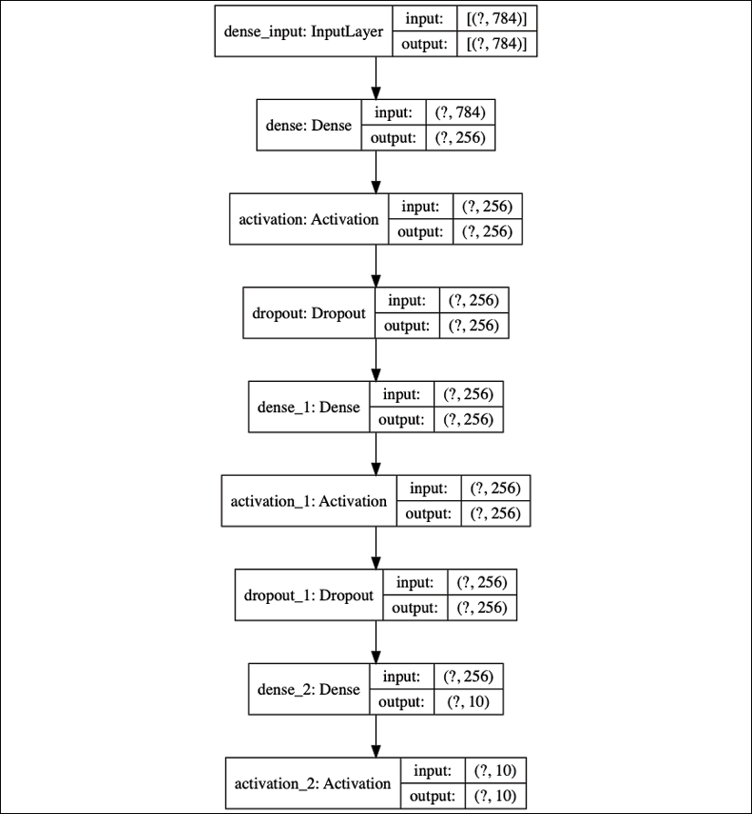
Figure 1.3.9: The graphical description of the MLP MNIST digit classifier
Having summarized our model, this concludes our discussion of MLPs. In the next section, we will build a MNIST digit classifier model based on CNN.
4. Convolutional Neural Network (CNN)
We are now going to move onto the second artificial neural network, CNN. In this section, we're going to solve the same MNIST digit classification problem, but this time using a CNN.
Figure 1.4.1 shows the CNN model that we'll use for the MNIST digit classification, while its implementation is illustrated in Listing 1.4.1. Some changes in the previous model will be needed to implement the CNN model. Instead of having an input vector, the input tensor now has new dimensions (height, width, channels) or (image_size, image_size, 1) = (28, 28, 1) for the grayscale MNIST images. Resizing the train and test images will be needed to conform to this input shape requirement.

Figure 1.4.1: The CNN model for MNIST digit classification
Implement the preceding figure:
Listing 1.4.1: cnn-mnist-1.4.1.py
import numpy as np
from tensorflow.keras.models import Sequential
from tensorflow.keras.layers import Activation, Dense, Dropout
from tensorflow.keras.layers import Conv2D, MaxPooling2D, Flatten
from tensorflow.keras.utils import to_categorical, plot_model
from tensorflow.keras.datasets import mnist
# load mnist dataset
(x_train, y_train), (x_test, y_test) = mnist.load_data()
# compute the number of labels
num_labels = len(np.unique(y_train))
# convert to one-hot vector
y_train = to_categorical(y_train)
y_test = to_categorical(y_test)
# input image dimensions
image_size = x_train.shape[1]
# resize and normalize
x_train = np.reshape(x_train,[-1, image_size, image_size, 1])
x_test = np.reshape(x_test,[-1, image_size, image_size, 1])
x_train = x_train.astype('float32') / 255
x_test = x_test.astype('float32') / 255
# network parameters
# image is processed as is (square grayscale)
input_shape = (image_size, image_size, 1)
batch_size = 128
kernel_size = 3
pool_size = 2
filters = 64
dropout = 0.2
# model is a stack of CNN-ReLU-MaxPooling
model = Sequential()
model.add(Conv2D(filters=filters,
                 kernel_size=kernel_size,
                 activation='relu',
                 input_shape=input_shape))
model.add(MaxPooling2D(pool_size))
model.add(Conv2D(filters=filters,
                 kernel_size=kernel_size,
                 activation='relu'))
model.add(MaxPooling2D(pool_size))
model.add(Conv2D(filters=filters,
                 kernel_size=kernel_size,
                 activation='relu'))
model.add(Flatten())
# dropout added as regularizer
model.add(Dropout(dropout))
# output layer is 10-dim one-hot vector
model.add(Dense(num_labels))
model.add(Activation('softmax'))
model.summary()
plot_model(model, to_file='cnn-mnist.png', show_shapes=True)
# loss function for one-hot vector
# use of adam optimizer
# accuracy is good metric for classification tasks
model.compile(loss='categorical_crossentropy',
              optimizer='adam',
              metrics=['accuracy'])
# train the network
model.fit(x_train, y_train, epochs=10, batch_size=batch_size)
_, acc = model.evaluate(x_test,
                        y_test,
                        batch_size=batch_size,
                   verbose=0)
print("
Test accuracy: %.1f%%" % (100.0 * acc))
The major change here is the use of the Conv2D layers. The ReLU activation function is already an argument of Conv2D. The ReLU function can be brought out as an Activation layer when the batch normalization layer is included in the model. Batch normalization is used in deep CNNs so that large learning rates can be utilized without causing instability during training.
Convolution
If, in the MLP model, the number of units characterizes the Dense layers, the kernel characterizes the CNN operations. As shown in Figure 1.4.2, the kernel can be visualized as a rectangular patch or window that slides through the whole image from left to right, and from top to bottom. This operation is called convolution. It transforms the input image into a feature map, which is a representation of what the kernel has learned from the input image. The feature map is then transformed into another feature map in the succeeding layer and so on. The number of feature maps generated per Conv2D is controlled by the filters argument.

Figure 1.4.2: A 3 × 3 kernel is convolved with an MNIST digit image.
The convolution is shown in steps tn and tn+1 where the kernel moved by a stride of 1 pixel to the right.
The computation involved in the convolution is shown in Figure 1.4.3:

Figure 1.4.3: The convolution operation shows how one element of the feature map is computed
For simplicity, a 5 × 5 input image (or input feature map) where a 3 × 3 kernel is applied is illustrated. The resulting feature map is shown after the convolution. The value of one element of the feature map is shaded. You'll notice that the resulting feature map is smaller than the original input image, this is because the convolution is only performed on valid elements. The kernel cannot go beyond the borders of the image. If the dimensions of the input should be the same as the output feature maps, Conv2D accepts the option padding='same'. The input is padded with zeros around its borders to keep the dimensions unchanged after the convolution.
Pooling operations
The last change is the addition of a MaxPooling2D layer with the argument pool_size=2. MaxPooling2D compresses each feature map. Every patch of size pool_size × pool_size is reduced to 1 feature map point. The value is equal to the maximum feature point value within the patch. MaxPooling2D is shown in the following figure for two patches:

Figure 1.4.4: MaxPooling2D operation. For simplicity, the input feature map is 4 × 4, resulting in a 2 × 2 feature map.
The significance of MaxPooling2D is the reduction in feature map size, which translates to an increase in receptive field size. For example, after MaxPooling2D(2), the 2 × 2 kernel is now approximately convolving with a 4 × 4 patch. The CNN has learned a new set of feature maps for a different receptive field size.
There are other means of pooling and compression. For example, to achieve a 50% size reduction as MaxPooling2D(2), AveragePooling2D(2) takes the average of a patch instead of finding the maximum. Strided convolution, Conv2D(strides=2,…), will skip every two pixels during convolution and will still have the same 50% size reduction effect. There are subtle differences in the effectiveness of each reduction technique.
In Conv2D and MaxPooling2D, both pool_size and kernel can be non-square. In these cases, both the row and column sizes must be indicated. For example, pool_ size = (1, 2) and kernel = (3, 5).
The output of the last MaxPooling2D operation is a stack of feature maps. The role of Flatten is to convert the stack of feature maps into a vector format that is suitable for either Dropout or Dense layers, similar to the MLP model output layer.
In the next section, we will evaluate the performance of the trained MNIST CNN classifier model.
Performance evaluation and model summary
As shown in Listing 1.4.2, the CNN model in Listing 1.4.1 requires a smaller number of parameters at 80,226 compared to 269,322 when MLP layers are used. The conv2d_1 layer has 640 parameters because each kernel has 3 × 3 = 9 parameters, and each of the 64 feature maps has one kernel and one bias parameter. The number of parameters for other convolution layers can be computed in a similar way.
Listing 1.4.2: Summary of a CNN MNIST digit classifier
Layer (type)	                 Output Shape	        Param #
=================================================================
conv2d_1 (Conv2D)                (None, 26, 26, 64)      640
max_pooling2d_1 (MaxPooiling2)   (None, 13, 13, 64)      0
conv2d_2 (Conv2D)                (None, 11, 11, 64)      36928
max_pooling2d_2 (MaxPooiling2)   (None, 5.5, 5, 64)      0
conv2d_3 (Conv2D)                (None, 3.3, 3, 64)      36928
flatten_1 (Flatten)              (None, 576)             0
dropout_1 (Dropout)              (None, 576)             0
dense_1 (Dense)                  (None, 10)              5770
activation_1 (Activation)        (None, 10)              0
===================================================================
Total params: 80,266
Trainable params: 80,266
Non-trainable params: 0
Figure 1.4.5: shows a graphical representation of the CNN MNIST digit classifier.
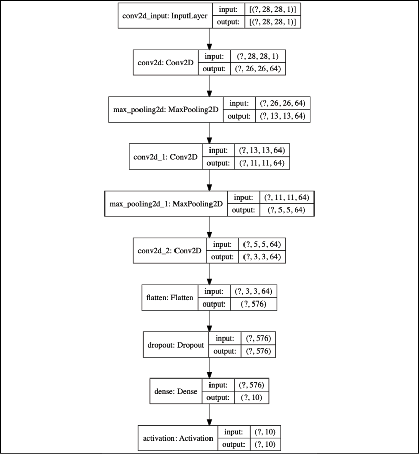
Figure 1.4.5: Graphical description of the CNN MNIST digit classifier
Table 1.4.1 shows a maximum test accuracy of 99.4%, which can be achieved for a 3-layer network with 64 feature maps per layer using the Adam optimizer with dropout=0.2. CNNs are more parameter efficient and have a higher accuracy than MLPs. Likewise, CNNs are also suitable for learning representations from sequential data, images, and videos.
| Layers | Optimizer | Regularizer | Train Accuracy (%) | Test Accuracy (%) |
|
64-64-64 |
SGD |
Dropout(0.2) |
97.76 |
98.50 |
|
64-64-64 |
RMSprop |
Dropout(0.2) |
99.11 |
99.00 |
|
64-64-64 |
Adam |
Dropout(0.2) |
99.75 |
99.40 |
|
64-64-64 |
Adam |
Dropout(0.4) |
99.64 |
99.30 |
Table 1.4.1: Different CNN network configurations and performance measures for the CNN MNIST digit classifier.
Having looked at CNNs and evaluated the trained model, let's look at the final core network that we will discuss in this chapter: RNN.
5. Recurrent Neural Network (RNN)
We're now going to look at the last of our three artificial neural networks, RNN.
RNNs are a family of networks that are suitable for learning representations of sequential data like text in natural language processing (NLP) or a stream of sensor data in instrumentation. While each MNIST data sample is not sequential in nature, it is not hard to imagine that every image can be interpreted as a sequence of rows or columns of pixels. Thus, a model based on RNNs can process each MNIST image as a sequence of 28-element input vectors with timesteps equal to 28. The following listing shows the code for the RNN model in Figure 1.5.1:

Figure 1.5.1: RNN model for MNIST digit classification
Listing 1.5.1: rnn-mnist-1.5.1.py
import numpy as np
from tensorflow.keras.models import Sequential
from tensorflow.keras.layers import Dense, Activation, SimpleRNN
from tensorflow.keras.utils import to_categorical, plot_model
from tensorflow.keras.datasets import mnist
# load mnist dataset
(x_train, y_train), (x_test, y_test) = mnist.load_data()
# compute the number of labels
num_labels = len(np.unique(y_train))
# convert to one-hot vector
y_train = to_categorical(y_train)
y_test = to_categorical(y_test)
# resize and normalize
image_size = x_train.shape[1]
x_train = np.reshape(x_train,[-1, image_size, image_size])
x_test = np.reshape(x_test,[-1, image_size, image_size])
x_train = x_train.astype('float32') / 255
x_test = x_test.astype('float32') / 255
# network parameters
input_shape = (image_size, image_size)
batch_size = 128
units = 256
dropout = 0.2
# model is RNN with 256 units, input is 28-dim vector 28 timesteps
model = Sequential()
model.add(SimpleRNN(units=units,
                    dropout=dropout,
                    input_shape=input_shape))
model.add(Dense(num_labels))
model.add(Activation('softmax'))
model.summary()
plot_model(model, to_file='rnn-mnist.png', show_shapes=True)
# loss function for one-hot vector
# use of sgd optimizer
# accuracy is good metric for classification tasks
model.compile(loss='categorical_crossentropy',
              optimizer='sgd',
              metrics=['accuracy'])
# train the network
model.fit(x_train, y_train, epochs=20, batch_size=batch_size)
_, acc = model.evaluate(x_test,
                        y_test,
                        batch_size=batch_size,
                        verbose=0)
print("
Test accuracy: %.1f%%" % (100.0 * acc))
There are two main differences between the RNN classifier and the two previous models. First is the input_shape = (image_size, image_size), which is actually input_ shape = (timesteps, input_dim) or a sequence of input_dim-dimension vectors of timesteps length. Second is the use of a SimpleRNN layer to represent an RNN cell with units=256. The units variable represents the number of output units. If the CNN is characterized by the convolution of kernels across the input feature map, the RNN output is a function not only of the present input but also of the previous output or hidden state. Since the previous output is also a function of the previous input, the current output is also a function of the previous output and input and so on. The SimpleRNN layer in Keras is a simplified version of the true RNN. The following equation describes the output of SimpleRNN:
 (Equation 1.5.1)
In this equation, b is the bias, while W and U are called recurrent kernel (weights for the previous output) and kernel (weights for the current input), respectively. Subscript t is used to indicate the position in the sequence. For a SimpleRNN layer with units=256, the total number of parameters is 256 + 256 × 256 + 256 × 28 = 72,960, corresponding to b, W, and U contributions.
The following figure shows the diagrams of both SimpleRNN and RNN when used for classification tasks. What makes SimpleRNN simpler than an RNN is the absence of the output values ot = Vht + c before the softmax function is computed:

Figure 1.5.2: Diagram of SimpleRNN and RNN
RNNs might be initially harder to understand when compared to MLPs or CNNs. In an MLP, the perceptron is the fundamental unit. Once the concept of the perceptron is understood, an MLP is just a network of perceptrons. In a CNN, the kernel is a patch or window that slides through the feature map to generate another feature map. In an RNN, the most important is the concept of self-loop. There is in fact just one cell.
The illusion of multiple cells appears because a cell exists per timestep, but in fact it is just the same cell reused repeatedly unless the network is unrolled. The underlying neural networks of RNNs are shared across cells.
The summary in Listing 1.5.2 indicates that using a SimpleRNN requires a fewer number of parameters.
Listing 1.5.2: Summary of an RNN MNIST digit classifier
Layer (type)	               Output Shape	  Param #
=================================================================
simple_rnn_1 (SimpleRNN)       (None, 256)        72960
dense_1 (Dense)                (None, 10)         2570
activation_1 (Activation)      (None, 10)         36928
=================================================================
Total params: 75,530
Trainable params: 75,530
Non-trainable params: 0
Figure 1.5.3 shows the graphical description of the RNN MNIST digit classifier. The model is very concise:

Figure 1.5.3: The RNN MNIST digit classifier graphical description
Table 1.5.1 shows that the SimpleRNN has the lowest accuracy among the networks presented:
| Layers | Optimizer | Regularizer | Train Accuracy (%) | Test Accuracy (%) |
|
256 |
SGD |
Dropout(0.2) |
97.26 |
98.00 |
|
256 |
RMSprop |
Dropout(0.2) |
96.72 |
97.60 |
|
256 |
Adam |
Dropout(0.2) |
96.79 |
97.40 |
|
512 |
SGD |
Dropout(0.2) |
97.88 |
98.30 |
Table 1.5.1: The different SimpleRNN network configurations and performance measures
In many deep neural networks, other members of the RNN family are more commonly used. For example, Long Short-Term Memory (LSTM) has been used in both machine translation and question answering problems. LSTM addresses the problem of long-term dependency or remembering relevant past information to the present output.
Unlike an RNN or a SimpleRNN, the internal structure of the LSTM cell is more complex. Figure 1.5.4 shows a diagram of LSTM. LSTM uses not only the present input and past outputs or hidden states, but it introduces a cell state, st, that carries information from one cell to the other. The information flow between cell states is controlled by three gates, ft, it, and qt. The three gates have the effect of determining which information should be retained or replaced and the amount of information in the past and current input that should contribute to the current cell state or output. We will not discuss the details of the internal structure of the LSTM cell in this book. However, an intuitive guide to LSTMs can be found at http://colah.github.io/posts/2015-08-Understanding-LSTMs.
The LSTM() layer can be used as a drop-in replacement for SimpleRNN(). If LSTM is overkill for the task at hand, a simpler version called a Gated Recurrent Unit (GRU) can be used. A GRU simplifies LSTM by combining the cell state and hidden state together. A GRU also reduces the number of gates by one. The GRU() function can also be used as a drop-in replacement for SimpleRNN().

Figure 1.5.4: Diagram of LSTM. The parameters are not shown for clarity.
There are many other ways to configure RNNs. One way is making an RNN model that is bidirectional. By default, RNNs are unidirectional in the sense that the current output is only influenced by the past states and the current input.
In bidirectional RNNs, future states can also influence the present and past states by allowing information to flow backward. Past outputs are updated as needed depending on the new information received. RNNs can be made bidirectional by calling a wrapper function. For example, the implementation of bidirectional LSTM is Bidirectional(LSTM()).
For all types of RNNs, increasing the number of units will also increase the capacity. However, another way of increasing the capacity is by stacking the RNN layers. It should be noted though that as a general rule of thumb, the capacity of the model should only be increased if needed. Excess capacity may contribute to overfitting, and, as a result, may lead to both a longer training time and a slower performance during prediction.
6. Conclusion
This chapter provided an overview of the three deep learning models – MLP, RNN, CNN – and also introduced TensorFlow 2 tf.keras, a library for rapid development, training, and testing deep learning models that is suitable for a production environment. The Sequential API of Keras was also discussed. In the next chapter, the Functional API will be presented, which will enable us to build more complex models specifically for advanced deep neural networks.
This chapter also reviewed the important concepts of deep learning such as optimization, regularization, and loss functions. For ease of understanding, these concepts were presented in the context of MNIST digit classification.
Different solutions to MNIST digit classification using artificial neural networks, specifically MLP, CNN, and RNN, which are important building blocks of deep neural networks, were also discussed together with their performance measures.
With an understanding of deep learning concepts and how Keras can be used as a tool with them, we are now equipped to analyze advanced deep learning models. After discussing the Functional API in the next chapter, we'll move on to the implementation of popular deep learning models. Subsequent chapters will discuss selected advanced topics such as autoregressive models (autoencoder, GAN, VAE), deep reinforcement learning, object detection and segmentation, and unsupervised learning using mutual information. The accompanying Keras code implementations will play an important role in understanding these topics.
7. References
- Chollet, François. Keras (2015). https://github.com/keras-team/keras.
- LeCun, Yann, Corinna Cortes, and C. J. Burges. MNIST handwritten digit database. AT&T Labs [Online]. Available: http://yann.lecun.com/exdb/mnist2 (2010).