
CHAPTER 2
SYSTEM DYNAMICS AND MODELS
The performance of estimation algorithms is highly dependent on the accuracy of models. Model development is generally the most difficult task in designing an estimator. The equations for least squares and Kalman filtering are well documented, but proper selection of system models and parameters requires a good understanding of the system and of various trade-offs in selecting model structure and states. We start by discussing dynamic and measurement models. This provides the reader with a better understanding of the problem when estimation algorithms are presented in later chapters.
Chapter 1 was deliberately vague about the structure of models because the intent was to present concepts. The dynamic (time evolution) model of the true system used in Figure 1.1 was a generic form. The system state vector x(t) was an n-element linear or nonlinear function of various constant parameters p, known time-varying inputs u(τ) defined over the time interval t0 ≤ τ ≤ t, random process noise q(τ) also defined over the time interval t0 ≤ τ ≤ t, and possibly time, t:
Function ft was defined as a time integral of the independent variables. The m-element measurement vector y(t) was assumed to be a function of x(t) with additive random noise:
(2.0-2)
![]()
However, these models are too general to be useful for estimation. We now consider the options. Models are first divided into two categories: continuous and discrete. Nearly all practical implementations of the Kalman filter use the discrete filter form. The continuous filter developed by Kalman and Bucy is useful for analytic purposes, but it is rarely implemented because most physical systems are discretely sampled. Nonetheless, continuous models are important because the majority of discrete least-squares and Kalman filter applications are based on integration of a continuous system model. Continuous time models generally take one of the following forms:
1. An expansion in time using basis functions such as polynomials, Fourier series, or wavelets.
2. A derivation from first-principle (e.g., physical, thermodynamic, chemical, biological) concepts. This may lead to distributed models based on partial differential equations, or lumped-parameter (linear or nonlinear) models based on ordinary differential equations.
3. A stochastic random process model (e.g., random walk, Markov process) to model effects that are poorly understood or behave randomly.
4. Combinations of the above.
5. Linear regression models.
Kalman (1960) and Kalman and Bucy (1961) assumed that discrete dynamic system models could be obtained as the time integral of a continuous system model, represented by a set of first-order ordinary differential equations. If continuous system models are obtained as high-order ordinary differential equations, they can be converted to a set of first-order ordinary differential equations. Hence Kalman’s assumption is not restrictive.
The first category of continuous models—basis function expansion—multiplies the basis functions by coefficients that are included in the state vector of estimated parameters. The model itself is not a function of other parameters and hence is nonparametric. The second and third categories (except for random walk) depend on internal parameters and are thus parametric. The model parameters must be determined before the model can be used for estimation purposes.
Discrete models are based on the assumption that the sampling interval is fixed and constant. Discrete process models are parametric, and may take the following forms:
1. Autoregressive (AR)
2. Moving average (MA)
3. Autoregressive moving average (ARMA)
4. Autoregressive moving average with exogenous inputs (ARMAX)
5. Autoregressive integrated moving average (ARIMA)
Each of these model types is discussed below and in Appendix D (available online at ftp://ftp.wiley.com/public/sci_tech_med/least_squares/). We start the discussion with discrete dynamic models since they are somewhat simpler and the ultimate goal is to develop a model that can be used to process discretely sampled data.
2.1 DISCRETE-TIME MODELS
Discrete models can be viewed as a special case of continuous system models where measurements are sampled at discrete times, and system inputs are held constant over the sampling intervals. Discrete models assume that the sampling interval T is constant with no missing measurements, and that the system is a stationary random process such that the means and autocorrelation functions do not change with time shifts (see Appendix B). These conditions are often found in process control and biomedical applications (at least for limited time spans), and thus ARMAX models are used when it is difficult to derive models from first principles. Empirical computation of these models from sampled data is discussed in Chapter 12.
The general form of a single-input, single-output, n–th order ARMAX process model is
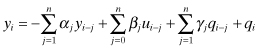
where
| yi | is the sampled measurement at time ti, |
| ui | is the exogenous input at time ti, |
| qi | is zero-mean random white (uncorrelated) noise input at time ti, and ti − ti−1 = T for all i. |
The summations for yi−j, ui−j, and qi−j in equation (2.1-1) may be separately truncated at lower order than n. Alternate forms of the general model are defined as follows.
1. If all αj = 0 and βj = 0, the model is MA because the output measurement is a weighted average of past noise inputs qi−j.
2. If all γj = 0 and βj = 0, the model is AR because the output measurement is a weighted average of past measurements and the current noise input qi.
3. If all βj = 0, the model is ARMA because exogenous inputs are not included.
The z-transform transfer function of an ARMA model is
(2.1-2)
![]()
where z−1 is the unit delay operator,
![]()
![]() and f is frequency in Hz. The transfer function can be factored to obtain
and f is frequency in Hz. The transfer function can be factored to obtain
where
(2.1-4)
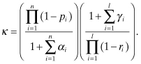
The zeroes, ri, and poles, pi, may be real or complex. Complex poles or zeroes must occur in complex conjugate pairs for a real system. Hence equation (2.1-3) can be written in terms of first-order factors for real poles and zeroes, and second-order factors for complex conjugate poles or zeroes. For example, the transfer function for complex conjugate pole (p, p*) and zero (r, r*) pairs can be written as
(2.1-5)
where Re(·) and Im(·) are the real and imaginary parts of the complex number, and |·|2 = Re(·)2 + Im(·)2. If the roots of the denominator (poles) all lie within the unit circle in the complex plane, the model is stable (output remains bounded) and causal (output only depends on past inputs, not future). If all poles and zeroes (roots of the numerator) are inside the unit circle it is called a minimum phase or invertible system, because the input noise qi can be reconstructed from knowledge of the past outputs yj for j ≤ i.
Since qi is assumed to be white
(uncorrelated) noise, the power spectral density (PSD)
of qi is the same at all frequencies:![]()
The PSD versus frequency of the real output yi can be computed as
(2.1-6)
![]()
where Y(z) is the z-transform of yi. Since an AR process does not have zeroes, it is called an all-pole model and is best applied to systems that have spectral peaks. An MA process is an all-zero model best applied to systems with spectral nulls. ARMA models can handle both spectral nulls and peaks.
Multi-input, multi-output ARMAX models are usually represented using state-space models of the form
(2.1-7)
![]()
or
(2.1-8)
![]()
where xi is an n-element state vector, qi is a p-element process noise vector, ui is an l-element input vector, yi is an m-element measurement vector, and ri is an m-element measurement noise vector. The various arrays are defined accordingly.
Measured outputs of many systems have nonzero means, trends, or other types of systematic long-term behavior. When successive differences of measurements result in a stationary process, the system may be treated as an ARIMA process. Box et al. (2008, chapter 4) discuss different approaches for handling nonstationary processes.
Appendix D explains AR, MA, ARMA, ARMAX, and ARIMA models in greater detail and includes examples. It also shows how discrete models can be derived from continuous, linear state space models that are discretely sampled. However, it is usually not practical to compute the model parameters αi, βi, and λi directly from a continuous model. Chapter 12 discusses methods for determining the parameters empirically from measured data.
To summarize, discrete models can be used when the sampling interval and types of measurements are fixed, and the system is statistically stationary and linear. With extensions they can also be used for certain types of nonstationary or nonlinear systems. Discrete models are often used in applications when it is difficult to develop a model from first principles. For example, they are sometimes used in process control (Åström 1980; Levine 1996) and biomedical (Lu et al. 2001; Guler et al. 2002; Bronzino 2006) applications.
2.2 CONTINUOUS-TIME DYNAMIC MODELS
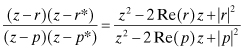
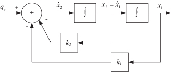
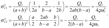
Continuous time dynamic models are usually defined by a set of linear or nonlinear first-order differential state equations. Differential equations are linear if coefficients multiplying derivatives of the dependent variable x are not functions of x. The assumption of first-order differential equations is not restrictive since higher order differential equations can be written as a set of first-order equations. For example, the stochastic linear second-order system
![]()
can be written as![]()
A block diagram of the model is shown in Figure 2.1.
FIGURE 2.1: Stochastic second-order dynamic model.
In the general case the state differential equations may be nonlinear:
where x, u, and qc are all a function of time. As before, x and f are n-element vectors, u is an l-element vector of control inputs, and qc is a p-element white noise vector. Notice that function f in equation (2.2-1) is assumed to be a function of the state x rather than the parameter vector p used in equation (2.0-1). We have implicitly assumed that all unknown parameters in p are included in the system state vector x. Other parameters in p that are known with a high degree of accuracy are treated as part of the model and are thus ignored in our generic model equation.
It should be noted that white noise has infinite power, so inclusion of white noise input in a differential equation is not physically realistic. Furthermore, integration of the differential equation is not defined in the usual sense, even when f(x,u,qc,t) is linear. The problem is briefly described in Appendix B. Jazwinski (1970), Schweppe (1973), Åström (1970), and Levine (1996, chapters 34, 60) provide more extended discussions of calculus for stochastic processes. For estimation purposes we are usually interested in expectations of stochastic integrals, and for most continuous functions of interest, these integrals can be treated as ordinary integrals. This assumption is used throughout the book.
In many cases the function f is time-invariant, but we will not yet apply this restriction. Since process noise qc(t) is assumed to be zero mean and a small perturbation to the model, it is customary to assume that superposition applies. Thus the effect can be modeled as an additive linear term
where the n × p matrix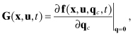
is possibly a
nonlinear function of x. For nonlinear models, most
least-squares or Kalman estimation techniques numerically integrate ![]() (without qc since it is zero mean) to
obtain the state vector x at the measurement times.
However, least-squares and Kalman estimation techniques also require the sensitivity
of x(ti), where
ti is a measurement time, with respect to
x(te), where
te is the epoch time. This sensitivity is
required when computing the optimal weighting of the data, and it is normally
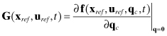
computed as a linearization of the nonlinear equations. That is, equation (2.2-1) is expanded in a Taylor
series about a reference trajectory and only the linear terms are retained:
(without qc since it is zero mean) to
obtain the state vector x at the measurement times.
However, least-squares and Kalman estimation techniques also require the sensitivity
of x(ti), where
ti is a measurement time, with respect to
x(te), where
te is the epoch time. This sensitivity is
required when computing the optimal weighting of the data, and it is normally
computed as a linearization of the nonlinear equations. That is, equation (2.2-1) is expanded in a Taylor
series about a reference trajectory and only the linear terms are retained:
where
| δx = x(t) − xref(t), δu = u(t) − uref(t) xref(t) and uref(t) |
are the reference trajectory, |
|
|
is an n × n matrix, |
|
|
is an n × l matrix, |
|
is an n × p matrix. |
Sources for reference trajectories will be discussed in later chapters. The perturbation equation (2.2-3), without the qc term, is integrated to obtain the desired sensitivities. If the model is entirely linear, the model becomes:
This linear form is assumed in the next section, but it is recognized that the methods can be applied to equation (2.2-3) with suitable redefinition of terms.
2.2.1 State Transition and Process Noise Covariance Matrices
To obtain a state model at discrete measurement times ti, i = 1, 2,…, the continuous dynamic models of equation (2.2-2), (2.2-3), or (2.2-4) must be time-integrated over intervals ti to ti+1. For a deterministic linear system, the solution can be represented as the sum of the response to an initial condition on x(ti), called the homogeneous solution, and the response due to the driving (forcing) terms u(t) and q(t) for ti < t ≤ ti+1, called the particular or forced solution, that is,
(2.2-5)
![]()
The initial condition solution is defined as the response of the
homogeneous differential equation ![]() or
or
![]() :
:
In many applications equation (2.2-6) is numerically integrated using truncated Taylor series, Runge-Kutta, or other methods. Numerical integration can also be used to compute effects of the control u(t) if it is included in f(x(λ),u(λ),λ) of equation (2.2-6). However, a more analytic method is needed to compute the sensitivity matrix (either linear sensitivity or partial derivatives) of x(ti+1) with respect to x(ti). It will be seen later that this sensitivity matrix is required to calculate the optimal weighting of measurement data for either least-squares or Kalman estimation. It is also necessary to characterize—in a covariance sense—the effect of the random process noise qc(t) over the time interval ti to ti+1 when computing optimal weighting in a Kalman filter.
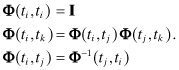
The state sensitivity is provided by the state transition matrix Φ(ti+1,ti), implicitly defined from
for a linear system. A similar equation applies for linearized
(first-order) state perturbations in a nonlinear system,![]()
but Φ is
then a function of the actual state x(t) over the time interval ti to
ti+1. This nonlinear case will
be addressed later. For the moment we assume that the linear equation (2.2-7) applies. From equation (2.2-7), it can be seen that
(2.2-8)
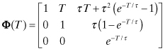
When F(t) is time-invariant (F(t) = F), the solution is
obtained as for the scalar problem ![]() ,
which has the solution x(ti+1) = efT
x(ti) with T = ti+1 − ti. Hence
,
which has the solution x(ti+1) = efT
x(ti) with T = ti+1 − ti. Hence
(2.2-9)
![]()
The exponential can be represented as an infinite Taylor series
(2.2-10)
![]()
which is sometimes useful when evaluating Φ(T). Other methods will be presented in Section 2.3.
In the general linear case where F(t) is time-varying, the solution is more complicated. If F(t) satisfies the commutativity condition
then it can be shown (DeRusso et al. 1965, p. 363) that
(2.2-12)
![]()
Unfortunately equation (2.2-11) is rarely satisfied when systems are time-varying (including cases where the system is nonlinear and Φ has been computed as a linearization about the reference trajectory). Analytic techniques have been developed to compute Φ when commutativity does not exist (DeRusso et al. 1965, pp. 362–366), but the methods are difficult to implement for realistic problems. More generally, the relationship
is true for both time-varying and time-invariant cases. This can be
derived by differentiating equation (2.2-7) with respect to time, substituting the homogeneous part of equation
(2.2-4) for ![]() , and substituting equation (2.2-7) for xH(ti+1). Thus equation (2.2-13) may be numerically integrated to obtain Φ(ti+1,ti).
More will be said about this in Section 2.3.
, and substituting equation (2.2-7) for xH(ti+1). Thus equation (2.2-13) may be numerically integrated to obtain Φ(ti+1,ti).
More will be said about this in Section 2.3.
Assuming that Φ(ti+1,ti) can be computed, the total solution x(ti+1) for the model equation (2.2-4) is
where
(2.2-15)
![]()
and
Notice that the particular solution (including the effects of u(t) and qc(t)) is computed as convolution integrals involving Φ(ti+1,λ). If the system dynamics represented by F(t) are time-invariant, then equations (2.2-14) to (2.2-16) will use Φ(ti+1 − ti) and Φ(ti+1 − λ). As noted before, most nonlinear applications compute the portion of x(ti+1) due to x(ti) and u(t) by direct numerical integration, but even in these cases equation (2.2-16) is used when calculating the covariance of qc(t).
Some elements of uD and qD may be zero if the indicated integrals do not affect all states, but that detail is ignored for the moment. We now concentrate on qD. The continuous process noise qc(t) is assumed to be random: for modeling purposes it is treated as unknown and cannot be directly integrated to compute qD. It is also assumed that qc(t) is zero-mean (E[qc(t)] = 0) white noise with known PSD matrix Qs:
(2.2-17)
![]()
where E[·] denotes expected value and δ(t − τ) is the Dirac delta function. Since
is unitless, δ(t) must have units of inverse time, such as 1/s. Hence Qs must have units of (magnitude)2·s. For example, if the i-th element of qc(t) directly drives a state having units of volts, then the diagonal (i,i) element of Qs must have units of volts2·s or volts2/Hz. Thus Qs is a PSD.
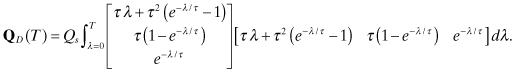
Using equation (2.2-16), the covariance of qD is computed as:

Since ![]() for t ≠ τ and qc(t)
is the only variable within the integral that is random, the expectation may be
moved within a single integral:
for t ≠ τ and qc(t)
is the only variable within the integral that is random, the expectation may be
moved within a single integral:

where we have defined the discrete process noise covariance
(2.2-21)
![]()
Notice that
![]()
for ti ≠ tj because ![]() for t ≠ τ, and no sample
of qc(t) is common to both intervals ti−1 < t ≤
ti and tj−1 < t ≤
tj. Furthermore E[qD(ti,ti)] = 0 for all
ti because E[qc(t)] = 0.
for t ≠ τ, and no sample
of qc(t) is common to both intervals ti−1 < t ≤
ti and tj−1 < t ≤
tj. Furthermore E[qD(ti,ti)] = 0 for all
ti because E[qc(t)] = 0.
At first glance equation (2.2-20) may not appear very useful because the “messy” convolution integral involves products of the state transition matrix, and we have indicated that computation of Φ(t,τ) may not be trivial. You may wonder why QD is needed at all. For least-squares applications QD is zero because the model is deterministic. However, QD is used in the Kalman filter to compute optimal weighting of measurement data. Fortunately QD can be approximated because the covariance equations used to compute weighting need not be as accurate as the state model. This will be discussed again in Chapter 8.
Before considering various methods for computing the state transition and process noise covariance matrices, we first discuss the types of dynamic models that may be used in estimation problems.
2.2.2 Dynamic Models Using Basic Function Expansions
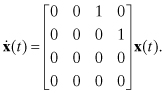
The simplest type of dynamic model treats the measurement data as an expansion in basis functions. This is really just curve fitting using a constraint on the type of fit. Polynomials are probably the most commonly used basis function. For example, a scalar measurement could be represented as a third-order polynomial in time
(2.2-22)
![]()
where c0, c1 , c2, and c3 are the polynomial coefficients. If the deterministic model is used in least-squares estimation, the epoch model states can be set equal to the coefficients:
(2.2-23)
![]()
Since the states are constant, the dynamic model is simply x(t) = x(0) and the measurement equation is
(2.2-24)
![]()
However, if the model is to be used in a Kalman filter with process noise driving the states, it is usually better to define the measurement using a moving epoch for the state:
![]()
where
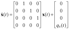
and the initial state is![]()
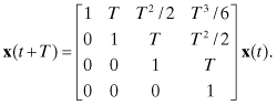
Equation (2.2-25), without the effect of q4(t), is integrated over the time interval between measurements, T, to obtain:
(2.2-26)
The extension to include the effect of process noise (q4(t) in this example) will be addressed later when discussing random process models.
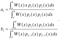
One problem in using polynomials for least-squares fitting is the tendency of the solution to become numerically indeterminate when high-order terms are included. The problem of numerical singularity and poor observability is discussed further in Chapter 5. To minimize numerical problems, it is often advisable to switch from ordinary polynomials to polynomials that are orthogonal over a given data span (see Press et al. 2007, section 4.5). Two functions are considered orthogonal over the interval a ≤ x ≤ b with respect to a given weight function W(x) if
(2.2-27)
![]()
A set of mutually orthogonal functions fi(x), i = 1, 2, … , n is called orthonormal if ![]() for all i. A set of orthogonal
polynomials pi(x)
for j = 0, 1, 2,… can be constructed using the
recursions
for all i. A set of orthogonal
polynomials pi(x)
for j = 0, 1, 2,… can be constructed using the
recursions
(2.2-28)

where
(2.2-29)
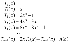
As one example, Chebyshev polynomials are orthogonal over the interval
−1 to 1 for a weight of ![]() . They are
defined by
. They are
defined by
(2.2-30)
![]()
or explicitly
(2.2-31)
Notice that to use Chebyshev polynomials over an arbitrary interval a ≤ y ≤ b, the affine transformation
![]()
must be applied. Unlike ordinary polynomials, Chebyshev polynomials are bounded by −1 to +1 for all orders. Hence the numerical problems of ordinary polynomials, caused by large values of high-order terms, are avoided when using orthogonal polynomials. Use of orthonormal transformations to minimize the effects of numerical errors is discussed in later chapters, and there is a connection between these orthonormal transformations and orthonormal polynomials.
Other possibilities for basis functions include Fourier series and wavelets. In deciding which function to use, consider the characteristics. Polynomials can accurately model smooth functions and trends, but high-order models are needed to follow abrupt changes. Fourier expansions are ideal for functions that are periodic over a finite data span, but do not model trends well unless linear and quadratic terms are added. Wavelets are useful for modeling nonperiodic functions that have limited time extent (Press et al. 2007, section 13.10). Notice that the measurement data span used for the modeling should be limited so that the basis function expansion can accurately model data within the span. If the span is long, it may be necessary to carry many terms in the expansion, and this could cause problems if the model is used to predict data outside the measurement data span: the prediction will tend to rapidly diverge when high-order terms are included in the data fits.
Example 2.1: GOES Instrument “Attitude”
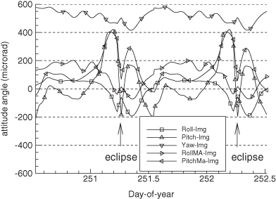
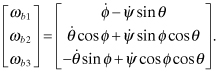
Basis function modeling can be used not only for curve fitting, but also for modeling a physical system when it is difficult to develop a first-principles model. For example, a combination of a polynomial and Fourier series expansions is used to model imaging instrument misalignments on the GOES I-P spacecraft (Gibbs 2008). The GOES geosynchronous weather satellites provide continuous images of the western hemisphere from a nearly equatorial position and fixed longitude. Because imaging instruments have small internal misalignments, the optical boresight at various scan angles is modeled using five misalignment parameters: three Euler attitude rotations (roll, pitch, and yaw) and two lumped-parameter misalignments. The five misalignments vary with time because instrument thermal deformation is driven by solar heating. Since the spacecraft has a fixed position with respect to the earth, the angle of the sun relative to the spacecraft has a pattern that nearly repeats every day. Thus misalignments have a fundamental period equal to the solar day. The misalignment profile is not exactly sinusoidal so it is necessary to include harmonics of the 24-h period to model the fine structure. For GOES, each of the five misalignment parameters is modeled as the sum of a linear or quadratic term plus a Fourier series of 4 to 13 harmonics, depending on the parameter. For example, instrument roll ϕ(t) is modeled as
![]()
where θ = 2π t/1440 and t is minutes of the solar day. The other four misalignment parameters are modeled similarly using different x coefficients. Then the instrument-observed scan angles to various stars and landmarks are modeled using a nonlinear function of the five misalignment angles. Least-squares estimation is used to determine the epoch misalignment states, so the state dynamic model is simply x(t) = x(0) with the time variation of the five misalignment parameters included in the measurement model.
Figure 2.2 shows the estimated GOES-13 Imager misalignment angles over a 48-h period that includes eclipses at approximately Greenwich Mean Time (GMT) days 251.25 and 252.25 in 2006. Eclipse periods lasting a maximum of 72 min at the spring and autumnal equinoxes have a significant effect on instrument temperatures and thus misalignment angles. Instrument thermal recovery can take several hours after eclipse end, so “eclipse periods” of 4 h are modeled separately from the normal 24-h model.
FIGURE 2.2: Estimated Imager misalignments for GOES-13 during eclipse season 2006.
2.2.3 Dynamic Models Derived from First Principles
When working with physical systems, it is usually better to develop models from first principles, rather than computing empirical models from measured data only. The first-principles approach has the potential advantage of greater accuracy and the ability to model an extended (nontested) range of operating conditions. It also has the potential disadvantages of poor estimation accuracy if the model structure or parameters are incorrect, and development of good first-principle models may be difficult for some systems. A standard approach uses first-principles models for parts of the system that are well modeled, and then includes random walk or Markov process (colored noise) models for parts of the system (usually higher order derivatives) that appear to be random or have uncertain characteristics. If it is difficult to develop a first-principles model, or if the model uncertainty is great, then a totally empirical approach may be better. This is discussed in Chapter 12.
It is important to understand all relevant physical laws, the assumptions on which those laws are based, and the actual conditions existing in the system to be modeled when developing first-principles models. You will need to either work with an expert or become an expert yourself. However, beware—system experts tend to focus on the subject that they know best and sometimes create detailed models that include effects irrelevant for estimation purposes. For example, it is generally unnecessary and undesirable to model high-frequency effects not observed at the measurement sampling rate. These effects can often be treated as process or measurement noise. Calibration of simulation models based on an expert’s instinct rather than measured data is another problem. This author has received models that exhibited physically impossible behavior because model parameters were not properly calibrated. Thus the best approach may be to work closely with an expert, but consider carefully when deciding on effects or parameters to be modeled in the estimation.
This book does not attempt to discuss all types of first-principles modeling—that would be a formidable task. Rather, we summarize the main modeling concepts and demonstrate the modeling of physical systems by a few examples. More examples are provided in Chapter 3 and Appendix C. The goal is to present concepts and guidelines that can be generally applied to estimation problems. Be warned, however, that the listed equations may not be directly applicable to other problems, so consult references and check the assumptions before using them. More information on model building and identification may be found in Fasol and Jörgl (1980), Levine (1996), Balchen and Mummé (1988), Close et al. (2001), Isermann (1980), Ljung and Glad (1994), Ljung (1999) and Åström (1980).
Typical “first-principles” concepts used in model building include
1. Conservation of mass: for example, the continuity equation
2. Conservation of momentum: for example, Newton’s laws of motion
3. Conservation of energy: for example, first law of thermodynamics
4. Second law of thermodynamics and entropy relationships
5. Device input/output relationships: for example, pump, fan, motor, thruster, resistor, capacitor, inductor, diode, transistor
6. Flow/pressure relationships: for example, pipes, ducts, aerodynamics, porous media
7. Heat transfer models: for example, conductive, convective, radiant
8. Chemical reactions: for example, combustion thermodynamics
9. Optical properties and relationships
10. Special and general relativity.
This list is obviously not exhaustive as many other “first principles” exist. Use of these principles may lead to distributed models based on partial differential equations (PDE), or lumped-parameter (linear or nonlinear) models based on ordinary differential equations (ODE). When PDEs are used, boundary conditions must be specified. To simplify solutions, it is sometimes desirable to discretize a distributed model so that PDEs are replaced with ODEs. Models may be static, dynamic, or both. Other classifications include deterministic or stochastic, and parametric or nonparametric. Time delays—such as those resulting from mass transport—cannot be exactly represented as differential equations, so it may be necessary to explicitly model the delay or to approximate it using ODEs.
After structure of a parametric model is defined, the parameter values must be determined. In some cases component or subsystem test data may be available, and it may be possible to determine parameters directly from the data. In other cases data from a fully instrumented system must be used to identify parameters. Much has been written about this subject, and discussions may be found in previously listed references. Note that parameter observability is affected by the types of perturbing signals and the presence of control feedback.
The remainder of this section summarizes a few basic concepts that are often used in first-principles models. Other useful concepts are described in Appendix C and in listed references.
2.2.3.1 Linear Motion
Constant velocity motion is one of the most commonly used models for tracking applications. This often appears as the default for tracking of ships and aircraft since both vehicles move in a more-or-less straight line for extended periods of time. However, any tracker based on a constant velocity assumption must also include some means for detecting acceleration or sudden changes in velocity (when the interval between measurements is longer than the applied acceleration). In two lateral dimensions (x and y) where r denotes position and v denotes velocity, the state vector is xT = [rx ry vx vy], which has time derivative
(2.2-32)
This can be integrated to obtain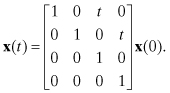
If used in a Kalman filter, process noise on the two velocity states should be modeled to account for occasional changes in velocity.
2.2.3.2 Linear Momentum Change
Newton’s second law is![]()
where f is the vector of applied
force, m is body mass, and v
is the velocity vector. This equation can be added to the linear motion model above.
If mass does not change and a known applied force is from an external source, the
two-dimensional model becomes
(2.2-33)
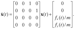
In other words, the applied force is treated as an exogenous input: u in equation (2.2-4). If no information on applied force is available, x and y acceleration should be included as “constant” states. If added at the bottom of the state vector, that is, x = [rx ry vx vy ax ay]T, the dynamic model becomes
(2.2-34)
In this case acceleration will not remain constant for long periods of time, so a Kalman filter should be used and process noise on the acceleration should be modeled. Alternately least-squares estimation could be used, but it would be necessary to include some mechanism for detecting changes in acceleration and re-initializing the estimate (Willsky and Jones 1974, 1976; Basseville and Benveniste 1986; Bar-Shalom and Fortmann 1988; Gibbs 1992).
A different choice of acceleration states may be appropriate in some cases. For example, both ships and aircraft tend to turn at an approximately constant angular rate. They also tend to accelerate along the current velocity vector when additional thrust is applied (or aircraft pitch is changed). When multiple measurements are available during the maneuvers, the estimator may perform better using constant crosstrack acceleration (ac) as state #5 and constant alongtrack acceleration (aa) as state #6. This leads to
(2.2-35)
![]()
where ![]() . Notice
that the model is now nonlinear, but the problems introduced by the nonlinearity may
be offset by the improved performance due to the better model. Chapter 9 includes an
example that uses this model in a Kalman filter. To implement this model in a
filter, the nonlinear equations are usually linearized about reference velocities to
obtain first-order perturbation equations, that is,
. Notice
that the model is now nonlinear, but the problems introduced by the nonlinearity may
be offset by the improved performance due to the better model. Chapter 9 includes an
example that uses this model in a Kalman filter. To implement this model in a
filter, the nonlinear equations are usually linearized about reference velocities to
obtain first-order perturbation equations, that is,![]()
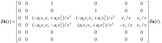
The perturbation form of this model is:
(2.2-36)
2.2.3.3 Rotational Motion
Rotational motion of a rigid body is described by
![]()
where τ is the applied torque and
h is the angular momentum vector measured in a
nonrotating coordinate system. If τ and h are referenced to the coordinate system of the rotating body (the
b-system), then hb
= Ibωb where Ib is the inertia
tensor of the body and ωb is the rotational rate. Since the reference frame is
rotating, the change in angular momentum of the rotating coordinate system must be
accounted for as part of the angular acceleration (Goldstein 1950, section 4-8;
Housner and Hudson 1959, p. 203), that is,![]()
Rearranging yields:
(2.2-37)

If the inertia tensor is assumed to be diagonal (generally not true), the body angular accelerations are computed as
(2.2-38)
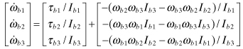
Notice that this model is nonlinear in ωb. If the body of interest contains other rotating bodies, such as momentum or reaction wheels, the separate angular momentum of those rotating bodies must be included as part of the total and additional states modeling the separate angular rates (or equivalently angular momentum) must be included. Depending upon how the model is structured, the “external torques” may include internal torques applied by motors connected to the momentum wheels. If the body of interest is an aircraft, aerodynamic forces (see Appendix C) and torques about the center-of-mass are computed for each section of the airframe and summed.
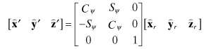
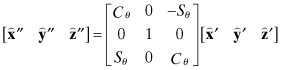
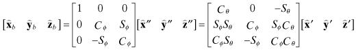
There are several choices for defining attitude. Euler angles are commonly used for representing aircraft attitude, and are sometimes used to define spacecraft attitude. If the Euler angles are defined in 3-2-1 order (as used for aircraft), the first rotation is about axis-3 (yaw or ψ), the next rotation is about axis-2 (pitch or θ), and the final rotation is about axis-1 (roll or ϕ). The rotation from the reference coordinates to the body coordinates can be represented as a direction cosine matrix:
(2.2-39)
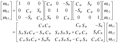
where Cθ = cos θ, Sθ = sin θ, etc. The rotation from body to the reference system is the transpose:
The body rates can be written in terms of the Euler angles rates by
direct resolution for the 3-2-1 rotation order. In the reference frame the body
rates are![]()
which map to the body frame
as
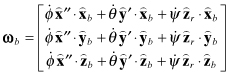
where
and ![]() ,
, ![]() ,
, ![]() are unit vectors defining the reference axes. Computation of
the vector dot products yields
are unit vectors defining the reference axes. Computation of
the vector dot products yields
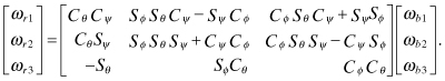
Equation (2.2-41) can be inverted to compute the Euler angle rates:
(2.2-42)
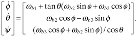
For computational reasons it is often preferable to order the states representing the highest derivatives at the end of the state vector. This tends to make the state transition matrix somewhat block upper triangular. Therefore we use ϕ, θ, ψ as the first three states and ωb1, ωb2, ωb3 as the last three states in the model.
There are several problems with the use of Euler angles as states.
First, the representation becomes singular when individual rotations equal 90
degrees. Hence they are mainly used for systems in which rotations are always less
than 90 degrees (such as for non-aerobatic aircraft). Further, the direction cosine
matrix and rotation require evaluation of six trigonometric functions and 25
multiplications; the computational burden makes that unattractive for evaluation
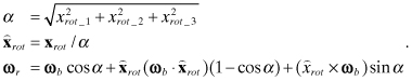
onboard spacecraft. For these reasons, most spacecraft use a quaternion
(4-parameter) representation for attitude rotations (Wertz 1978), or a similar
rotation vector model of the form ![]() where
where ![]() is the unit vector axis of
rotation and α is the angle of rotation. Then the
rotation from the body-to-reference system in equation (2.2-40) can be implemented as
is the unit vector axis of
rotation and α is the angle of rotation. Then the
rotation from the body-to-reference system in equation (2.2-40) can be implemented as
(2.2-43)
Notice that the rotation is implemented by summing vector components in three directions where the third vector is orthogonal to the first two. Two trigonometric functions, a square root, and 25 multiplications are still required in this implementation. The trig functions and square root are avoided when using an Euler-symmetric parameter (quaternion) representation (Wertz 1978, p. 414),
(2.2-44)
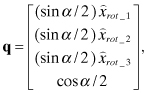
but extra computations are required to use the 4-parameter quaternion with a 3-state (first three quaternion parameters) model in a Kalman filter.
Appendix C summarizes other common first-principles models used for examples in this text.
2.2.4 Stochastic (Random) Process Models
Stochastic process models are frequently combined with other model types in Kalman filter applications to account for effects that are difficult to model or subject to random disturbances. These random models are typically used as driving terms for higher-order derivatives of the system model, although they can be used to drive any state.
2.2.4.1 Random Walk
The most commonly used random process model is the random walk, which is the discrete version of Brownian motion (also called a Wiener process). This is often used as a default model to account for time-varying errors when little information is available. The Brownian motion model is
where qc(t) is scalar white noise with![]()
Since the discrete state transition function (scalar) for equation (2.2-45) is Φ(T) = 1, the discrete process noise variance from equation (2.2-20) is
(2.2-46)
![]()
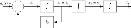
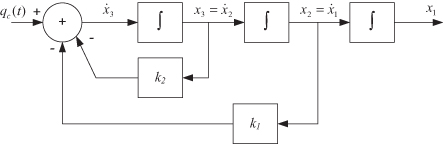
In other words, the variance of x increases linearly with the time interval for a random walk. A random walk model is often used as a driving term for the highest derivatives of the system, such as acceleration in a position/velocity/acceleration model. Hence we are interested in the integrated effect of the random walk on other states. Consider the three-state (position, velocity, acceleration) model
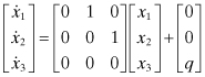
as shown in Figure 2.3.
FIGURE 2.3: Integrated Brownian motion.
The state transition matrix for this system is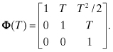
Hence the discrete state noise covariance of x(t + T) from equation (2.2-19) is

Equation (2.2-48) is very useful when trying to determine appropriate values for Qs since it is often easier to define appropriate values for the integrated effect of the process noise on other states. For example, we may have general knowledge that the integrated effect of acceleration process noise on position is about 10 m 1 − σ after a period of 1000 s. Hence we set Qs(1000)5/20 = 102 or Qs = 2 × 10⁻¹² m2/s5.
Although this example included white process noise on just the highest order state, this is not a general restriction: process noise can be included on any or all states. For example, one commonly used second-order clock error model includes process noise on both states:
(2.2-49)
![]()
where q1 and q2 are white noise and x2 is the clock timing error. Two separate q terms are used because clock errors have characteristics that can be approximated as both random walk and integrated random walk.
2.2.4.2 First-Order Markov Process (Colored Noise)
A first-order Markov process model is another commonly used random process model. A discrete or continuous stochastic process is called a Markov process if the probability distribution of a future state (vector) depends only on the current state, not past history leading to that state. This definition also includes random walk models. As with random walk models, low-order Markov process models are primarily used to drive the highest derivatives of the system dynamics, thus modeling correlated disturbing forces. In practice most Markov process models used for Kalman filters are first-order models, with second-order used occasionally. These low-order Markov process models are also called colored noise models because, unlike white noise, the PSD of the output is not constant with frequency. Most low-order Markov process implementations have “low-pass” characteristics because most of the power appears in the lowest frequencies.
A first-order Markov process is one in which the probability distribution of the scalar output depends on only one point immediately in the past, that is,
![]()
for every t1 < t2 < … < tk. The time-invariant stochastic differential equation defining a first-order Markov process model is
where τ is the model time constant and qc(t) is white noise. The state transition for equation (2.2-50) over time interval T is
(2.2-51)
![]()
and the discrete process noise variance is
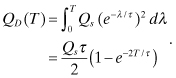
Unlike a random walk, a first-order Markov process has a steady-state
variance ![]() . Taking the limit of QD(T) as T → ∞ in equation (2.2-52),
. Taking the limit of QD(T) as T → ∞ in equation (2.2-52),
(2.2-53)
![]()
The inverse of this relationship, ![]() , is used when determining appropriate values of Qs given an approximate value of
, is used when determining appropriate values of Qs given an approximate value of ![]() . The autocorrelation function of the
steady-state process is
. The autocorrelation function of the
steady-state process is
(2.2-54)
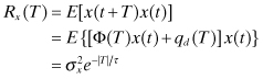
where qd(T) is the integrated effect of the process noise over the interval t to t + T and E[qd(T)x(t)] = 0. (See Appendix B for definitions of random process properties.) The PSD of a stationary random process can be computed as the Fourier transform of the autocorrelation function:
(2.2-55)
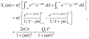
where ω = 2πf is frequency in radians/second. This obviously has the low-pass
characteristic mentioned previously. By moving the model output from the integrator
output to the integrator input, the PSD becomes![]()
which has a high-pass characteristic. This alternate model is seldom helpful in Kalman filter implementations because the Markov process output is generally passed through additional integrators in the system model. Hence the same effect can be obtained by moving the Markov process output to the input of an alternate system model state.
We now compute the state transition matrix and discrete state noise covariance for the same three-state system model used for the random walk model, but replace the third state random walk with a first-order Markov process, as shown in Figure 2.4.
FIGURE 2.4: Integrated first-order Markov process.
Using the property that ![]() (discussed later in Section 2.3) where s is a complex
variable,
(discussed later in Section 2.3) where s is a complex
variable, ![]() -1 is the inverse Laplace
transform and
-1 is the inverse Laplace
transform and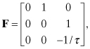
the state transition
matrix is computed as
and the discrete process noise covariance from equation (2.2-18) is
(2.2-57)
The (3,3) element of QD(T) is equal to![]()
which matches equation (2.2-52). Carrying out the indicated integration, the (1,1) and (2,2) elements are
(2.2-58)
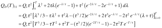
and
(2.2-59)
Notice that while the variance of the Markov process state x3 is constant, the variance of integrated Markov process states will increase with T, as for the random walk. However, the dominant exponent of T for state x1 is 3 (not 5) and the exponent of T for state x2 is 1 (not 3).
We leave integration of remaining terms as an exercise for the reader since most Kalman filter implementations that use first-order Markov process models only evaluate QD(T) for the Markov state. As discussed later in Section 2.3, elements of QD(T) for states that are integrals of the Markov state are usually approximations.
To summarize, the primary differences between the random walk model and the first-order Markov process model are
1. The variance of a first-order Markov process is constant in time. It increases linearly with time for a random walk.
2. The PSD of a first-order Markov process is nearly constant up to frequency 1/(2πτ) in Hz. Above this break frequency it falls off at −20 dB per decade. The PSD of white noise is constant at all frequencies. The PSD of a random walk process falls off at −20 dB per decade starting at 0 frequency.
3. The autocorrelation function of a first-order Markov process decays exponentially with the time shift. The autocorrelation function of white noise is zero for any nonzero time shift. The autocorrelation function of a random walk process is equal to 1 for all time shifts.
4. While the mean value of both processes is zero, a first-order Markov process will drive an initial condition towards zero. The initial state of a random walk is “remembered” indefinitely.
5. Because of the last property, physical states of a system model can be easily converted to random walk states by simply modeling the effect on the covariance of white noise added to the state differential equation. Use of a colored noise model, represented as a first-order Markov process, generally involves adding a state to the system model.
More on the pros and cons of using random walk and Markov processes for modeling system randomness appears after the discussion of second-order Markov processes.
2.2.4.3 Second-Order Markov Process
A second-order Markov process is a random process in which the probability distribution of the scalar output depends on only two output points immediately in the past, that is,
![]()
for every t1 < t2 < … < tk. Equivalently, the probability distribution of a two-state vector depends on only a single two-state vector immediately in the past. A time-invariant stochastic differential equation defining a second-order Markov process model is
where ω0 is the undamped natural frequency in radians/s and ς is the damping ratio (ς > 0). This can also be written as the two-state model:
(2.2-61)
![]()
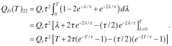
with state transition matrix
where ![]() , or
, or
where![]()
When 0 < ς < 1 the model is called underdamped because it tends to oscillate, and it is called overdamped when ς > 1. The critically damped case ς = 1 is handled differently since it has repeated roots. The results are listed in Gelb (1974, p. 44) and in Table 2.1 at the end of this section.
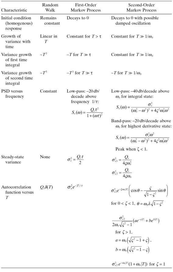
TABLE 2.1: Random Walk and Markov Process Characteristics
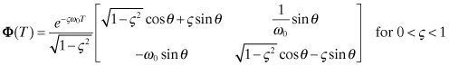
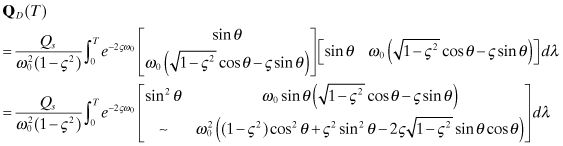
The discrete process noise covariance is
(2.2-64)
for 0 < ς < 1 with ![]() , or for ς
> 0,
, or for ς
> 0,
(2.2-65)
(Note: The symbol “∼” indicates that the term is equal to the transposed element, since the matrix is symmetric.) Carrying out the indicated integrations for the diagonal elements in the underdamped (0 < ς < 1) case gives the result
(2.2-66)
and
(2.2-67)
where ![]() . Taking
the limit as T → ∞, the steady-state variances of the
two states are
. Taking
the limit as T → ∞, the steady-state variances of the
two states are
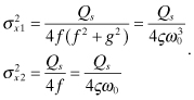
for 0 < ς < 1. ![]() can be used when determining
appropriate values of Qs given
can be used when determining
appropriate values of Qs given ![]() . Although not obvious, it can also be
shown that E[x1x2] = 0.
. Although not obvious, it can also be
shown that E[x1x2] = 0.
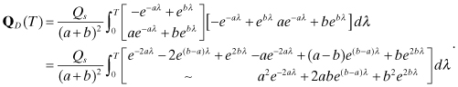
The equivalent relations for the overdamped case are
(2.2-69)
(2.2-70)
In the limit as T → ∞ the steady-state variances of the two states for ς > 0 are
(2.2-71)
As expected, these are the same equations as for the underdamped case (eq. 2.2-68). The autocorrelation function of the output state (x2) can be computed from the steady-state variance and Φ(T) using equation (2.2-62) or equation (2.2-63),
(2.2-72)
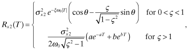
where a, b and θ were previously defined for equations (2.2-62) and (2.2-63).
The PSD of the output can be computed from the Laplace transform of the
transfer function corresponding to equation (2.2-60),![]()
which leads to
(2.2-73)
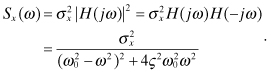
As expected, the PSD may exhibit a peak near ω0 when 0 < ς < 1. If the output is moved from the second to the first state, the PSD is
(2.2-74)
![]()
which has a band-pass characteristic.
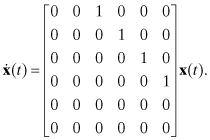
Low-order Markov process models are mostly used to account for randomness and uncertainty in the highest derivatives of a system model, so it is again of interest to characterize behavior of states that are integrals of the second-order Markov process output. Since the x1 state in equations (2.2-62) and (2.2-63) is equal to the integral of the model output (x2), x1 can be interpreted as proportional to velocity if x2 represents acceleration. Hence the integral of x1 can be interpreted as proportional to position. If we imbed the second-order Markov process in the three-state model used previously (for the random walk and first-order Markov process), and retain the state numbering used in equation (2.2-47) or (2.2-56), we obtain the integrated second-order Markov model of Figure 2.5.
FIGURE 2.5: Integrated second-order Markov process.
For this model the dynamic matrix F in ![]() is
is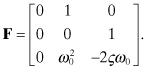
To compute the state transition matrix and discrete state noise
covariance of this model, we note that adding an extra integrator does not change
the dynamics of the second-order Markov process. Hence the lower-right 2 × 2 block
of Φ(t) will be equal to the
Φ(t) given in equation (2.2-62). Further, process noise
only drives the third state, so Φ(t)13 is the
only element of Φ(t) that is
required to compute the position (1,1) element of QD. We again use ![]() and obtain
and obtain
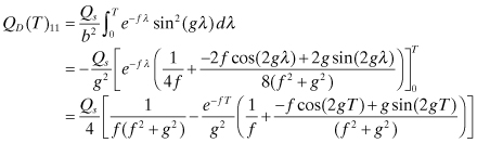
(2.2-75)
![]()
for 0 < ς < 1 with f = ςω0 and ![]() . This is used to compute
. This is used to compute
(2.2-76)
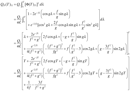
The point of this complicated derivation is to show that QD(T)11
grows linearly with T for T
![]() c (=ςω0).
c (=ςω0).
Figure 2.6 shows the PSD for
1. White noise process (integrated state is random walk)
2. First-order Markov process with f0 = 10 Hz
3. Second-order Markov process with ζ = 0.1 and f0 = 10 Hz
4. Second-order Markov process with ζ = 0.5 and f0 = 10 Hz
5. Second-order Markov process with ζ = 1.0 and f0 = 10 Hz
6. Second-order Markov process with ζ = 2.0 and f0 = 10 Hz
7. Second-order Markov process with ζ = 1.0, f0 = 10 Hz, and output at x3 in Figure 2.5
FIGURE 2.6: Normalized power spectral density of random process models.
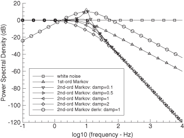
This is scaled by −20 dB to keep the PSD on the same plot as other data.
In all cases Qs = 1, but the PSD magnitudes were adjusted to be equal at frequency 0, except for case #7. Notice that both the first and second-order (x2 output) Markov processes have low-pass characteristics. Power falls off above the break frequency at −20 dB/decade for the first-order model and −40 dB/decade for the second-order model with x2 as output. The second-order Markov process using x3 as output has a band-pass characteristic and the PSD falls off at −20 dB/decade above 10 Hz. Also note that the second-order model has a peak near 10 Hz when 0 < ς < 1.
Table 2.1 compares the characteristics of the three random process models. When selecting a random process model for a particular application, pay particular attention to the initial condition response, the variance growth with time, and the PSD. Random walk models are used more frequently than Markov process models because they do not require additional states in a system model. Furthermore, measurements are often separated from the random process by one or two levels of integration. When measurement noise is significant and measurements are integrals of the driving process noise, it is often difficult to determine whether the process noise is white or colored. In these cases little is gained by using a Markov process model, rather than assuming white process noise for an existing model state.
When used, Markov process noise models are usually first-order. Second-order models are indicated when the PSD has a dominant peak. Otherwise, first-order models will usually perform as well as a second-order models in a Kalman filter. This author has only encountered three applications in which second-order Markov process models were used. One modeled motion of maneuvering tanks where tank drivers used serpentine paths to avoid potential enemy fire. The second application modeled a nearly oscillatory system, and the third modeled spacecraft attitude pointing errors.
2.2.5 Linear Regression Models
Least-squares estimation is sometimes referred to as regression modeling. The term is believed to have been first used by Sir Francis Galton (1822–1911) to describe his discovery that the heights of children were correlated with the parent’s deviation from the mean height, but they also tended to “regress” to the mean height. The coefficients describing the observed correlations with the parent’s height were less than one, and were called regression coefficients. As the term is used today, regression modeling usually implies fitting a set of observed samples using a linear model that takes into account known input conditions for each sample. In other words, it tries to determine parameters that represent correlations between input and output data. Hence the model is generally based on observed input-output correlations rather than on first-principle concepts. For example, regression modeling is used by medical researchers when trying to determine important parameters for predicting incidence of a particular disease.
To demonstrate the concept, assume that we are researching causative factors for lung cancer. We might create a list of potential explanatory variables that include:
1. Total years of smoking
2. Average number of cigarettes smoked per day
3. Number of years since last smoked
4. Total months of exposure to asbestos above some threshold
5. Urban/suburban/rural location
6. Type of job
7. Age
8. Gender
9. Race
10. Socioeconomic status.
This is not intended to be an exhaustive list but rather a sample of parameters that might be relevant. Then using a large sample of lung cancer incidence and patient histories, we could compute linear correlation coefficients between cancer incidence and the explanatory variables. The model is
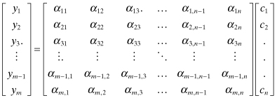
where
| yi | variables represent a particular person i’s status as whether (+1) or not (0) he/she had lung cancer, |
| αij | coefficients are person i’s response (converted to a numeric value) to a question on explanatory factor j, and |
| cj | coefficients are to be determined by the method of least squares. |
Additional αij coefficients could also include nonlinear functions of other αij coefficients—such as products, ratios, logarithms, exponentials, and square roots—with corresponding definitions for the added cj coefficients. This type of model is very different from the models that we have considered so far. It is not based on a model of a physical system and does not use time as an independent variable (although time is sometimes included). Further, the “measurements” yi can only have two values (0 or 1) in this particular example. Since measurement noise is not explicitly modeled, the solution is obtained by minimizing a simple (unweighted) sum-of-squares of residuals between the measured and model-computed yi. It is likely that many of the cj will be nearly zero, and even for factors that are important, the cj values will still be small.
This book does not directly address this type of modeling. Many books on the subject are available (e.g., Tukey 1977; Hoaglin et al. 1983; Draper and Smith 1998; Wolberg 2006). However, various techniques used in regression modeling are directly relevant to more general least-squares estimation, and will be discussed in Chapter 6.
2.2.6 Reduced-Order Modeling
In many estimation applications it is not practical to use detailed first-principles models of a system. For example, three-dimensional simulations of mass and energy flow in a system (e.g., atmospheric weather, subsurface groundwater flow) often include hundreds of thousands or even millions of nodes. Although detailed modeling is often of benefit in simulations, use of such a high-order model in an estimator is generally neither necessary nor desirable. Hence estimators frequently use reduced-order models (ROMs) of systems. This was essential for several decades after initial development of digital computers because storage and processing power were very limited. Even today it is often necessary because problem sizes have continued to grow as fast (if not faster) than computational capabilities.
The methods used to develop a ROM are varied. Some of the techniques are as follows.
1. Define subsystem elements using lumped-parameter models of overall input-output characteristics (e.g., exponential response model of a heat exchanger) rather than using detailed first-principles models.
2. Ignore high-frequency effects not readily detected at measurement sampling frequencies, or above the dominant dynamic response of the system. Increase the modeled measurement noise variance to compensate.
3. Use first- or second-order Markov processes in a Kalman filter to model time-correlated effects caused by small system discontinuities or other quasi-random behavior. Empirically identify parameters of the Markov processes using moderately large samples of system input-output data (see Chapter 11).
4. Treat some model states as random walk processes (model white noise input to the derivative) rather than modeling the derivative using additional states.
5. Use eigen analysis to define linear combinations of states that behave similarly and can be treated as a single transformed state.
6. Ignore small magnitude states that have little effect on more important states. Compensate with additional process noise.
7. Reduce the number of nodes in a finite-element or finite difference model, and account for the loss of accuracy by either increasing the modeled measurement noise variance, increasing the process noise variance or both.
Some of these techniques are used in examples of the next chapter. It is difficult to define general ROM modeling rules applicable to a variety of systems. Detailed knowledge and first-principles understanding of the system under consideration are still desirable when designing a ROM. Furthermore, extensive testing using real and simulated data is necessary to validate and compare models.
2.3 COMPUTATION OF STATE TRANSITION AND PROCESS NOISE MATRICES
After reviewing the different types of models used to describe continuous systems, we now address computation of the state transition matrix (Φ) and discrete state noise covariance matrix (QD) for a given time interval T = ti+1 − ti. Before discussing details, it is helpful to understand how Φ and QD are used in the estimation process because usage has an impact on requirements for the methods. Details of least-squares and Kalman estimation will be presented in later chapters, but for the purposes of this section, it is sufficient to know that the propagated state vector x must be computed at each measurement time (in order to compute measurement residuals), and that Φ and QD must be computed for the time intervals between measurements. In fully linear systems, Φ may be used to propagate the state x from one measurement time to the next. In these cases, Φ must be very accurate. Alternately, in nonlinear systems the state propagation may be performed by numerical integration, and Φ may only be used (directly or indirectly) to compute measurement partial derivatives with respect to the state vector at some epoch time. If Φ is only used for purposes of computing partial derivatives, the accuracy requirements are much lower and approximations may be used.
As noted in Section 2.2.1, Φ is required in linear or nonlinear least-squares estimation to define the linear relationship between perturbations in the epoch state vector at t0 and the integrated state vector at the measurement times; that is, δx(ti) = Φ(ti,t0)δx(t0). Φ is also used when calculating optimal weighting of the data. Usually Φ is only calculated for time intervals between measurements, and Φ for the entire interval from epoch t0 is obtained using the product rule:
As used in the Kalman filter, Φ defines the state perturbations from one measurement time to the next:
(2.3-2)
![]()
The process noise covariance ![]() models the integrated effects of random process noise over the
given time interval. Both Φ and QD are required when calculating
optimal weighting of the measurements. The above perturbation definitions apply both
when the dynamic model is completely linear, or is nonlinear and has been linearized
about some reference state trajectory. Thus we assume in the next section that the
system differential equations are linear.
models the integrated effects of random process noise over the
given time interval. Both Φ and QD are required when calculating
optimal weighting of the measurements. The above perturbation definitions apply both
when the dynamic model is completely linear, or is nonlinear and has been linearized
about some reference state trajectory. Thus we assume in the next section that the
system differential equations are linear.
2.3.1 Numeric Computation of Φ
Section 2.2 briefly discussed three methods for computing the state transition matrix, Φ(T), corresponding to the state differential equation
To those three we add five other methods for consideration. The options are listed below.
1. Taylor series expansion of eFT
2. Padé series expansion of eFT
3. Inverse Laplace transform of [sI − F]−1
4. Integration of ![]()
5. Matrix decomposition methods
6. Scaling and squaring (interval doubling) used with another method
7. Direct numeric partial derivatives using integration
8. Partitioned combinations of methods
We now explore the practicality of these approaches.
2.3.1.1 Taylor Series Expansion of eFT
When the state dynamics are time-invariant (F is constant) or can be treated as time-invariant over the integration interval, Φ(T) is equal to the matrix exponential eFT, which can be expanded in a Taylor series as:
(2.3-4)
![]()
When F is time varying, the integral
![]()
can sometimes be used, but the conditions under which this applies are
rarely satisfied. In the time-invariant case, the Taylor series is useful when the
series converges rapidly. For example, the quadratic polynomial model,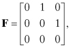
converges in two terms to
Full convergence in a few terms is unusual for real problems, but even so, numerical evaluation of the series can be used when “numeric convergence” is achieved in a limited number of terms. That is, the series summation is stopped when the additional term added is numerically insignificant compared with the existing sums. Moler and Van Loan (2003) compared methods for computing eA using a second-order example in which one eigenvalue of A was 17 times larger than the other. They found that 59 terms were required to achieve Taylor series convergence, and the result was only accurate to nine digits when using double precision. They generally regard series approximation as an inefficient method that is sensitive to round-off error and should rarely be used. Despite these reservations, Taylor series approximation for Φ(T) is sometimes used in the Kalman filter covariance time update because the covariance propagation can be less accurate than state vector propagation to achieve satisfactory performance in some cases. This statement will make more sense after reading Chapter 8 on the Kalman filter. In any case, use of series methods for computing Φ(T) is risky and should be considered only after numerically verifying that the approximation is sufficiently accurate for the given problem. Taylor series approximation of eA is used in MATLAB function EXPM2.
2.3.1.2 Padé Series Expansion of eFT
The (p,q) Padé approximation to eFT is
(2.3-5)
![]()
where
(2.3-6)

and
(2.3-7)

Matrix Dpq(FT)
will be nonsingular if p and q are sufficiently large or if the eigenvalues of FT are negative. Again, round-off error
makes Padé approximations unreliable. Cancellation errors can prevent accurate
determination of matrices N and D, or Dpq(FT)
may be poorly conditioned with respect to inversion. In Moler and Van
Loan’s second-order example described above, the best results were
obtained with p = q = 10,
and the condition number of D was greater than
104. All other values of p, q gave less accurate results. Use of p = q is generally more efficient and
accurate than p ≠ q.
However, Padé approximation to eFT can be used if
![]() FT
FT![]() is not too large (see Appendix A
for definitions of matrix norms). Golub and Van Loan (1996, p 572) present algorithm
11.3.1 for automatic selection of the optimum p, q to achieve a given accuracy. This algorithm combines
Padé approximation with the scaling and squaring method described below. Their
algorithm 11.3.1 is used in MATLAB function EXPM1.
is not too large (see Appendix A
for definitions of matrix norms). Golub and Van Loan (1996, p 572) present algorithm
11.3.1 for automatic selection of the optimum p, q to achieve a given accuracy. This algorithm combines
Padé approximation with the scaling and squaring method described below. Their
algorithm 11.3.1 is used in MATLAB function EXPM1.
2.3.1.3 Laplace Tranform
The Laplace transform of time-invariant differential equation (2.3-3) is
![]()
Hence the homogenous (unforced or initial condition) response can be
computed using the inverse Laplace transform as![]()
This implies that
(2.3-8)
![]()
This method was used in Section 2.2.4 when computing Φ for first- and second-order Markov processes. Notice that it involves analytically inverting the matrix [sI − F], computing a partial fractions expansion of each term in the matrix, and taking the inverse Laplace transform of each term. Even in the two-state case this involves much work, and the method is really not practical for manual computation when the state dimension exceeds four. However, the approach should be considered for low-order problems when analytic solutions are needed. It is also possible to implement Laplace transform methods recursively in software, or to use other approaches discussed by Moler and Van Loan. However, these methods are computationally expensive [O(n4)] and may be seriously affected by round-off errors.
2.3.1.4 Integration of ![]()
In Section 2.2.1 we showed that
(2.3-9)
![]()
for both time-varying and time-invariant models. Hence it is possible to
numerically integrate Φ over the time interval from t to τ, initialized with Φ(t, t) = I. Any general-purpose ODE numerical
integration method, such as fourth-order Runge-Kutta or Bulirsch-Stoer, employing
automatic step size control (see Press et al. 2007, chapter 17) may be used. To use
the ODE solver the elements of Φ must be stored in a vector and treated as a single
set of variables to be integrated. Likewise, the corresponding elements of ![]() must be stored in a vector and
returned to the ODE solver from the derivative function. This approach is easy to
implement and is relatively robust. However, there are a total of n2 elements in Φ for
an n-element state x, and
hence the numerical integration involves n2
variables if matrix structure is ignored. This can be computationally expensive for
large problems. At a minimum, the matrix multiplication FΦ
should be implemented using a general-purpose sparse matrix multiplication algorithm
(see Chapter 13) since F is often very sparse (as
demonstrated for the polynomial case). In some real-world problems F is more than 90% zeroes! If properly implemented, the
number of required floating point operations for the multiplication can be reduced
from the normal n3 by the fractional number
of nonzero entries in F, for example, nearly 90% reduction
for 90% sparseness. If it is also known that Φ has a
sparse structure (such as upper triangular), the number of variables included in the
integration can be greatly reduced. This does require, however, additional coding
effort. The execution time may be further reduced by using an ODE solver that takes
advantage of the linear, constant coefficient nature of the problem. See Moler and
Van Loan for a discussion of options. They also note that ODE solvers are
increasingly popular and work well for stiff problems.
must be stored in a vector and
returned to the ODE solver from the derivative function. This approach is easy to
implement and is relatively robust. However, there are a total of n2 elements in Φ for
an n-element state x, and
hence the numerical integration involves n2
variables if matrix structure is ignored. This can be computationally expensive for
large problems. At a minimum, the matrix multiplication FΦ
should be implemented using a general-purpose sparse matrix multiplication algorithm
(see Chapter 13) since F is often very sparse (as
demonstrated for the polynomial case). In some real-world problems F is more than 90% zeroes! If properly implemented, the
number of required floating point operations for the multiplication can be reduced
from the normal n3 by the fractional number
of nonzero entries in F, for example, nearly 90% reduction
for 90% sparseness. If it is also known that Φ has a
sparse structure (such as upper triangular), the number of variables included in the
integration can be greatly reduced. This does require, however, additional coding
effort. The execution time may be further reduced by using an ODE solver that takes
advantage of the linear, constant coefficient nature of the problem. See Moler and
Van Loan for a discussion of options. They also note that ODE solvers are
increasingly popular and work well for stiff problems.
2.3.1.5 Matrix Decomposition Methods
These are based on similarity transformations of the form F = SBS−1, which leads to
(2.3-10)
![]()
A transformation based on eigenvector/eigenvalue decomposition works well when F is symmetric, but that is rarely the case for dynamic systems of interest. Eigenvector/eigenvalue decomposition also has problems when it is not possible to compute a complete set of linearly independent eigenvectors—possibly because F is nearly singular. Other decompositions include the Jordan canonical form, Schur decomposition (orthogonal S and triangular B), and block diagonal B. Unfortunately, some of these approaches do not work when F has complex eigenvalues, or they fail because of high numerical sensitivity. Moler and Van Loan indicate that modified Schur decomposition methods are still of interest, but applications using this approach are rare. MATLAB function EXPM3 implements an eigenvector decomposition method.
2.3.1.6 Scaling and Squaring
The scaling and squaring (interval doubling) method is based on the observation that the homogenous part of x can be obtained recursively as
(2.3-11)
![]()
or
(2.3-12)
![]()
Hence the transition matrix for the total time interval T can be generated as
(2.3-13)
![]()
where m is an integer to be chosen.
Since Φ is only evaluated for the relatively small time
interval T/m, methods such
as Taylor series or Padé approximation can be used. If m
is chosen so that ![]() , a Taylor or Padé
series can be truncated with relatively few terms. (This criterion is equivalent to
selecting T/m to be small
compared with the time constants of F.) The method is also
computationally efficient and is not sensitive to errors caused by a large spread in
eigenvalues of F. However, it can still be affected by
round-off errors.
, a Taylor or Padé
series can be truncated with relatively few terms. (This criterion is equivalent to
selecting T/m to be small
compared with the time constants of F.) The method is also
computationally efficient and is not sensitive to errors caused by a large spread in
eigenvalues of F. However, it can still be affected by
round-off errors.
For efficient implementation, m should be chosen as a power of 2 for which Φ(T/m) can be reliably and efficiently computed. Then Φ(T) is formed by repeatedly squaring as follows:
![]()
![]()
![]()
![]()
![]()
![]()
where Tmax is the
maximum allowed step size, which should be less than the shortest time constants of
F. Notice that the doubling method only involves ![]() matrix multiplications.
matrix multiplications.
The scaling and squaring method has many advantages and is often used for least-squares and Kalman filtering applications. Since the time interval for evaluation of Φ is driven by the time step between measurements, scaling and squaring is only needed when the measurement time step is large compared with system time constants. This may happen because of data gaps or because availability of measurements is determined by sensor geometry, as in orbit determination problems. In systems where the measurement time interval is constant and small compared with system time constants, there is little need for scaling and squaring. Fortunately, many systems use measurement sampling that is well above the Nyquist rate. (The sampling rate of a continuous signal must be equal or greater than two times the highest frequency present in order to uniquely reconstruct the signal: see, for example, Oppenheim and Schafer, 1975.)
2.3.1.7 Direct Numeric Partial Derivatives Using Integration
Great increases in digital computer speeds during the last decades have allowed another option for calculation of Φ that would not have been considered 30 years ago: direct evaluation of numeric partial derivatives via integration. That is, from equation (2.3-1),
(2.3-14)
![]()
which works for both linear and nonlinear models. Hence each component j of x(t) can be individually perturbed by some small value, and x(t) can be numerically integrated from t to t + T. The procedure below shows pseudo-code that is easily converted to Fortran 90/95 or MATLAB:
![]()
![]()
![]()
![]()
![]()
![]()
![]()
![]()
![]()
Notice that central differences are used in the algorithm. You may wonder why they are preferred to one-sided differences since this doubles computations. The primary reason is that one-sided differences cannot be relied upon as accurate, regardless of the selected perturbation δx. This can be explained by personal experiences of the author (described below).
In the 1970s and early 1980s, this author routinely checked complicated derivations of analytic partial derivatives using numeric differences. Occasionally it was discovered that analytic and numeric partials did not agree within acceptable tolerances, and it was assumed that a mistake had been made in deriving or coding the analytic partials. Sometimes that was the case, but in several instances no error could be found even after hours of checking. It was eventually realized that errors in the one-sided (forward difference) numeric partials caused the discrepancy. No value of δx could be found for which the agreement between analytic and numeric partials was acceptable. When the numerical partials were changed to central differences, the agreement between the two methods was very good for δx values varying by orders of magnitude. This experience was repeated for several different problems that had little in common. Use of central differences cancels even terms in the Taylor series, and these terms are important down to the levels at which double precision round-off errors are important. Because of this experience, the author has only used central-differences for numerical partial derivatives computed since that time. Also, because of the robustness of central-difference numeric partials, the author has largely abandoned analytic partials for all but the simplest models, or systems in which the extra computational time of numeric partials cannot be tolerated. Use of numeric partials has the added advantage that the system model can be easily modified without having to re-derive analytic partials for the modified system. This makes the code much more flexible.
The primary problem in using numeric partial derivatives is selection of
the δx magnitude. A simple
rule suggested by Dennis and Schnabel (1983, p. 97) and Press et al. (2007, pp.
229–231) for simple functions and one-sided numeric derivatives in the absence of further information is
that δxi should be about one-half of the
machine accuracy εm. That is, the
perturbation δxi should be about ![]() . For double precision on a PC, εm = 2−53 = 1.1 × 10⁻¹⁶
in IEEE T_floating format, so
. For double precision on a PC, εm = 2−53 = 1.1 × 10⁻¹⁶
in IEEE T_floating format, so ![]() . For
central differences, δxi should be about
. For
central differences, δxi should be about ![]() . This step size minimizes the sum of
numerical rounding errors and Taylor series truncation errors.
. This step size minimizes the sum of
numerical rounding errors and Taylor series truncation errors.
However, the simple rule has several problems. First, xi could be nominally zero, so the perturbation
would then be zero. Hence the rule for central differences should be modified to![]()
where xnom_i is a
user-specified nominal magnitude for xi. A
second problem is that complicated functions can have relative errors much larger
than the machine accuracy. Hence the rule is modified to replace εm with εf, the relative accuracy of the computed function.
Unfortunately εf is often unknown, so εm is used by default. A third problem (related
to the second) for computing Φ is that differences in
magnitude and sensitivity of one state to another may be large. For example, in
geosynchronous orbit determination, the earth-centered-inertial (ECI) x and y coordinates of
satellite position will behave approximately as sinusoids with a magnitude of about
42,164 km. If the solar radiation pressure coefficient, Cp, with a nominal magnitude of about 1 (dimensionless)
is included in the state vector, it is found that a perturbation of 10−8
in Cp only results in a change in position of
about 2 × 10⁻¹⁰ m over a time interval of 10 min, which is a typical
interval between measurements. Hence the relative change in position is 2 ×
10−10/42164000 = 5 × 10⁻¹⁸, which is much smaller than the
double precision machine precision! In other words, the computed numerical partial
derivative will always be zero. To overcome this problem, the perturbation for
central differences should be set so that
(2.3-15)
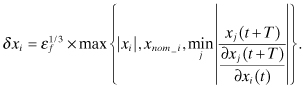
Unfortunately
![]()
will not be known in advance, so it is generally better to let the user define xnom_i such that it takes into account the sensitivity of other “measured states” to perturbations in xi.
Another approach defines xnom_i so that ![]() equals a small fraction, for example,
0.01 to 0.1, of the expected a-posteriori 1-σ
uncertainty (from the error covariance matrix) for the state. Recall that the
purpose of computing Φ is to iteratively calculate (for
nonlinear least-squares problems) perturbations in the estimate of the state x, where the iterations may continue until those
perturbations are small compared with the a-posteriori 1
− σ uncertainty. Hence the numeric partials must be
accurate for δxi perturbations of that
magnitude. Unfortunately the a-posteriori 1 − σ uncertainty will not be known until the estimation
software is coded and executed on real data. It is usually possible, however, to
guess the a-posteriori 1 − σ
uncertainty within a factor of 100. This is acceptable because numeric partials
computed using central differences are not sensitive to the exact perturbation δx, provided that it is
reasonable.
equals a small fraction, for example,
0.01 to 0.1, of the expected a-posteriori 1-σ
uncertainty (from the error covariance matrix) for the state. Recall that the
purpose of computing Φ is to iteratively calculate (for
nonlinear least-squares problems) perturbations in the estimate of the state x, where the iterations may continue until those
perturbations are small compared with the a-posteriori 1
− σ uncertainty. Hence the numeric partials must be
accurate for δxi perturbations of that
magnitude. Unfortunately the a-posteriori 1 − σ uncertainty will not be known until the estimation
software is coded and executed on real data. It is usually possible, however, to
guess the a-posteriori 1 − σ
uncertainty within a factor of 100. This is acceptable because numeric partials
computed using central differences are not sensitive to the exact perturbation δx, provided that it is
reasonable.
Further discussion of step size selection for numerical derivatives may be found in Dennis and Schnabel (1983, pp. 94–99), Vandergraft (1983, pp. 139–147), and Conte (1965, pp. 111–117).
Finally, we note that Φ can be obtained using numeric partial derivatives to compute
![]()
for the nonlinear system ![]() . Then Φ for the linearized system can be computed using
another method, such as Taylor series integration of
. Then Φ for the linearized system can be computed using
another method, such as Taylor series integration of ![]() .
.
2.3.1.8 Partitioned Combination of Methods
Some systems use both complex and simple dynamic models where the models are independent or loosely coupled. For example, it is not unusual in Kalman filters to have three types of states: core dynamic states, Markov process states, and bias dynamic states, with no coupling between Markov and bias as shown below:
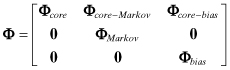
(Least-squares estimators do not include Markov process states since
they are not deterministic.) Φcore can be computed by one of the listed methods—most
likely Taylor series, integration of ![]() , scaling and squaring, or numeric partial derivatives. When dynamics are simple,
Φcore can
sometimes be computed analytically. ΦMarkov can be computed using the methods listed in
Section 2.2.4. Φbias is either the identity matrix or possibly an expansion
in basis functions. In many cases Φcore−Markov is approximated using low-order Taylor
series, because the Markov processes are usually treated as small-driving
perturbations in higher derivatives of the core states, moderate accuracy is
adequate if Φ is not used for propagating the state
vector. If higher accuracy is required, Φcore, ΦMarkov, and Φcore−Markov could be computed by integration of
, scaling and squaring, or numeric partial derivatives. When dynamics are simple,
Φcore can
sometimes be computed analytically. ΦMarkov can be computed using the methods listed in
Section 2.2.4. Φbias is either the identity matrix or possibly an expansion
in basis functions. In many cases Φcore−Markov is approximated using low-order Taylor
series, because the Markov processes are usually treated as small-driving
perturbations in higher derivatives of the core states, moderate accuracy is
adequate if Φ is not used for propagating the state
vector. If higher accuracy is required, Φcore, ΦMarkov, and Φcore−Markov could be computed by integration of
![]() . Likewise Φcore−bias could be computed by
the same methods used for Φcore−Markov, or if the bias terms just model measurement
errors, then Φcore−bias = 0.
. Likewise Φcore−bias could be computed by
the same methods used for Φcore−Markov, or if the bias terms just model measurement
errors, then Φcore−bias = 0.
Example 2.2: GOES I-P Orbit and Attitude Determination (OAD)
A simple example of this partitioning appears in the
batch least-squares OAD ground system software that supports the GOES I-P
geosynchronous weather imaging satellite (described in Example 2.1). Φcore models the
six spacecraft orbital dynamic states as described later in Chapter 3. Φbias = I since the biases are coefficients of the polynomial
and Fourier series expansions that model the time-varying instrument
“attitude” throughout the day. Since the two models are for
different physical systems, the state transition matrix is block diagonal; that
is, Φcore−bias
= 0. The two subsystems are coupled through the
measurement equations, not through dynamics. Because Φcore models complex orbital
forces, it is either computed using detailed (but approximate) analytic models
or using numerical partial derivatives. The time variation of the five
instrument attitude angles is computed as part of the measurement model, and
then the five angles—evaluated at the measurement times—are mapped to the
instrument scan angles of each observation: dy(t) = H(t)dx(t0) where![]()
Hence the measurement “dynamics” are included in the measurement model, not Φ. However, there is an option within OAD to include one force model bias—the solar radiation coefficient—as an estimated state. When this bias is estimated by OAD, the 6 × 1 Φcore−bias term is computed using an approximate analytic expression: essentially a first-order Taylor series.
The above methods for computing Φ are the principle ones used in estimation software. Moler and Van Loan list several other methods that could be used, but they also have problems. This author is not aware of estimation applications that use these alternate methods.
Notice that methods #4, #7, and possibly #8 are the only listed methods that can be directly used for time-varying systems. These “time-varying” systems include nonlinear systems when the system state x(t) changes significantly during the interval T so that the linearized
![]()
is not a good approximation to F(x(t + T)). In these cases, x(t) must be numerically integrated using m time steps of T/m (or non-equal steps), F(x) must be reevaluated at each intermediate value of x(t + jT/m), Φ(t + jT/m,t + (j − 1)T/m) must be recomputed for each value of F(x), and the total transition matrix must be computed as
(2.3-16)
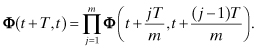
All the above methods are subject to a problem called the “hump”, but the problem particularly affects the scaling and squaring method. If the dynamics matrix F has eigenvalues that are close in magnitude and the off diagonal terms of F are large, then the magnitude of Φ(FT) = eFT may increase with T before it decreases. Moler and Van Loan give one example of this problem, repeated here in a slightly modified form with additional analysis.
Example 2.3: Hump in Computing Φ
For a two-element state, let
![]()
where a, b, and c are all positive. The system is stable since the eigenvalues (−a and −b) are negative. This is a realistic example in that F matrices for many physical systems have an approximately upper triangular structure and are stable. The problem occurs when c is large, and it can sometimes become worse when a is approximately, but not exactly, equal to b. Again this case is realistic for some real problems. Here Φ12 = c(e−aT − e−bT)/(b − a) and this term can become quite large. Figure 2.7 shows the four elements of Φ versus T for the case a = 1.152, b = 0.8682, and c = 10. Notice that Φ12 reaches a peak of 3.7 before decaying. Hence any round-off errors accumulated in computing Φ may grow as time increases to T = 1. If the scaling and squaring method is used to compute Φ with T/m < 1, the relative round-off errors may be magnified when computing Φ(T) = [Φ(T/m)]m.
Figure 2.8 shows the difference between the Φ elements computed using squaring and those computed from the exact solution
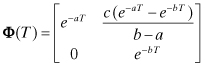
for the case where Φ(T/m) is computed using a fourth-order Taylor series in single precision (4 bytes) and Tmax = 0.2. Notice that the largest error is in Φ12 (as expected), and it exhibits a sawtooth characteristic that corresponds to changes in the number of squaring operations. The error grows with T/m since the dominant error is caused by truncation of the Taylor series to four terms. When an eight-order Taylor series is used, the error drops dramatically and becomes more random, as shown in Figure 2.9. In fact, no hump in error propagation is noticed when using an eight-order series. It appears that time growth of series truncation errors are influenced by the “hump” curve, but that round-off errors are not.
Table 2.2 summarizes the maximum Φ errors for various conditions. Notice that an eight-order series can achieve very high accuracy (1.9 × 10⁻¹⁰) using Tmax = 0.2 s with double-precision calculations, while in single precision calculations are limited to single-precision accuracy (1.7 × 10⁻⁶). There is little difference between single and double precision when using a fourth-order series since series truncation errors are the limiting factor. In this case, the maximum error is 2.0 × 10⁻⁴ for Tmax = 0.2 and 1.25 × 10⁻⁵ for Tmax = 0.1.
TABLE 2.2 Example 2.3 Error in Φ for Scaling and Squaring
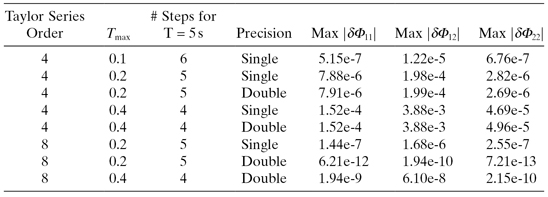
FIGURE 2.7: Φ versus T for Example 2.3.
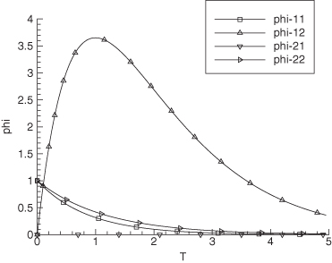
FIGURE 2.8: Error in Φ: fourth-order Taylor series, single precision, Tmax = 0.2.
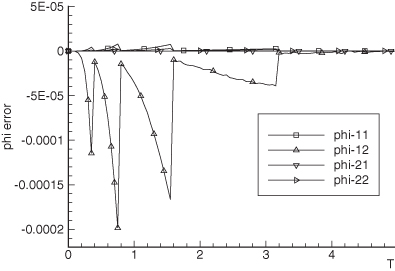
FIGURE 2.9: Error in Φ: eighth-order Taylor series, single precision, Tmax = 0.2.
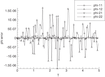
It is always risky to extrapolate results from simple examples to unrelated real-world problems. You should analyze error behavior for your particular problem before deciding on methods to be used. However, these results suggest that when using the scaling and squaring method for systems where growth of Φ follows a “hump,” it is important to minimize truncation errors by accurately computing Φ(T/m). Growth of round-off errors does not appear to follow a “hump” curve.
These results were obtained for a stable system, but many real systems include free integrators where elements of Φ grow almost linearly with time. In these cases, round-off error growth will be somewhat linear when using the scaling and squaring method, but growth of truncation errors may still follow sawtooth curves.
To summarize, truncated Taylor series, ODE integration of ![]() , numeric partials, scaling and
squaring, and combinations of these methods (possibly in partitions) are the primary
methods used for computing Φ in least-squares and Kalman
estimators. The series methods should only be used when the time step T is much less than shortest time constants (inverse
eigenvalues) of F. If the desired time step is larger than
the shortest time constants, then scaling and squaring (possibly with series
evaluation of the scaled Φ), integration of
, numeric partials, scaling and
squaring, and combinations of these methods (possibly in partitions) are the primary
methods used for computing Φ in least-squares and Kalman
estimators. The series methods should only be used when the time step T is much less than shortest time constants (inverse
eigenvalues) of F. If the desired time step is larger than
the shortest time constants, then scaling and squaring (possibly with series
evaluation of the scaled Φ), integration of ![]() , or numeric partials should be used.
For time-varying systems where it cannot be assumed that F
is constant during the integration interval, integration of
, or numeric partials should be used.
For time-varying systems where it cannot be assumed that F
is constant during the integration interval, integration of ![]() or numeric partials should be
used.
or numeric partials should be
used.
2.3.2 Numeric Computation of QD
Recall that the discrete state noise matrix QD is used in Kalman filters but not in least-squares estimators. Section 2.2.1 derived the equation for QD, repeated here:
where Qs = E[q(t)qT(t)] is the PSD of the continuous driving process noise q(t). When Φ is expressed analytically, it is sometimes possible to evaluate equation (2.3-17) analytically—this was demonstrated in Section 2.2.4 for low-order Markov processes. However, analytic evaluation is generally not an option for most applications. Fortunately Kalman filters work quite well using approximations for equation (2.3-17) because QD just accounts for the random error growth of the state x during time intervals between measurements. Provided that the time step T = ti+1 − ti is small compared with the time constants of F, these approximations usually involve expanding Φ in a zeroth, first- or second-order Taylor series, and then evaluating the integral equation (2.3-17). For a first-order expansion of Φ,
(2.3-18)
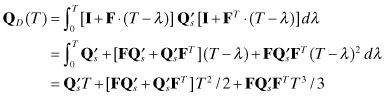
where for simplicity we have set ![]() . This equation is sometimes used to evaluate QD, but in many cases it is
simplified to
. This equation is sometimes used to evaluate QD, but in many cases it is
simplified to
![]()
or even just ![]() .
.
Since the accuracy of these approximations depend on the assumption that T is much less than smallest time constants of F, alternate methods must be available when the time step T between measurements is large—possibly because of data gaps. In these cases, Φ and QD should be evaluated in steps T/m where m is chosen so that T/m is small compared with shortest F time constants. This procedure works particularly well using the squaring method of the previous section. This can be derived using a time-invariant form of equation (2.2-13) with the u term ignored. The state propagation for two time steps is
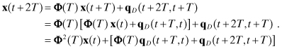
The last term in brackets is the total effect of process noise over the
interval t to t + 2T. We define it as qD2. We also define ![]() . Noting that because qs(t) is assumed to be stationary white noise,
. Noting that because qs(t) is assumed to be stationary white noise,
![]()
and![]()
Thus
(2.3-20)
![]()
This equation is valid regardless of the value of T, which suggests that the squaring technique listed previously for Φ can be modified to also include QD. The modified algorithm is
![]()
![]()
![]()
![]()
![]()
![]()
![]()
The iteration can be written so that arrays Φ and QD overwrite existing arrays at each iteration.
Finally we note one other option for computing QD, although it is rarely used. If we rewrite equation (2.3-19) as a general relationship for arbitrary times,
(2.3-21)
![]()
and then differentiate it with respect to time λ evaluated at time t, we obtain
where we have used ![]() and
and ![]() . Equation
(2.3-22) is a matrix Riccati equation. It can be integrated using a
general-purpose ODE solver, just as for
. Equation
(2.3-22) is a matrix Riccati equation. It can be integrated using a
general-purpose ODE solver, just as for ![]() . Note that it is only necessary to integrate the upper
triangular elements of the symmetric
. Note that it is only necessary to integrate the upper
triangular elements of the symmetric ![]() .
.
2.4 MEASUREMENT MODELS
Previous sections have concentrated on dynamic models because those are generally more difficult to develop than measurement models. Most measurements represent physical quantities where the functional relationship between measurements and model states is easily defined. For example, measurements in navigation problems (including orbit determination) are usually a nonlinear function of position and velocity. Examples include range, azimuth, elevation, and range rate from a sensor location to the target body-of-interest, or from the body-of-interest to another location or body.
An m-element vector of measurements y(t) is assumed to be modeled as a linear or nonlinear function of the state vector x(t) and random measurement noise r(t). For a nonlinear model,
(2.4-1)
![]()
or for a linear model
(2.4-2)
![]()
where H(t) is an m × n matrix that may be time-varying, and r(t) is an m-vector of zero-mean measurement noise. It is usually (but not always) assumed that r(t) is uncorrelated white noise with covariance R: E[r(t)rT(λ)] = Rδ(t − λ).
When the measurement equations are nonlinear, most least-squares or
Kalman filtering methods linearize the model about a reference xref (usually the current
estimate ![]() ) to develop perturbation
equations of the form
) to develop perturbation
equations of the form
(2.4-3)
![]()
where ![]()
Example 2.4: Range and Range-Rate Measurements
Measurements of range and range rate from a fixed site to a moving target are an example of a simple nonlinear model. The position vector of the sensor site is defined as ps = [psx psy psz]T and the position of the target is pt = [ptx pty ptz]T with velocity vt = [vtx vty vtz]T. The range from sensor to target is
(2.4-4)
![]()
and the range-rate is
(2.4-5)
![]()
If pt and vt are included in the state vector to be estimated, the measurement partial derivatives are
(2.4-6)
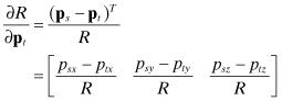
and
(2.4-7)
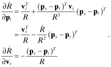
Most measurement sensors have inherent biases that may or may not be calibrated prior to use. Often the biases change with time, temperature, or other environmental parameters. Uncompensated measurement biases can have a very detrimental effect on the performance of the estimator. This is particularly true when multiple sensors each have their own biases. Hence it is important that either sensor biases be calibrated and biases removed from the measurements, or that the estimator include sensor biases in the state vector of adjusted parameters. Because of the time-varying nature of sensor “biases,” some sensors are routinely calibrated using data external to the normal measurements. For example, ground stations that track satellites or aircraft may calibrate range biases by periodically ranging to a ground transponder at a known location.
The measurement noise covariance matrix R is also a required input for the Kalman filter and weighted least-squares estimator. If the measurement sampling rate is much higher than the highest frequencies of the dynamic model, it is often possible to approximately determine the measurement noise variance by simply examining plots of the measurement data and calculating the variance about a smooth curve. One can also calculate the correlation between components of the measurement vector—such as range and range rate—using a similar approach. Time correlations (e.g., E[y(t)yT(t + λ)]) should be computed to determine whether the measurement errors are nearly time-independent, as often assumed. If time-correlation is significant, it will be necessary to account for this in the estimation as discussed later in Chapters 8.
In cases where measurement sampling rates are low or measurements are taken at infrequent intervals, other methods for determining R are needed. Sometimes the measurement sensor manufacturer will provide measurement error variances, but actual errors are often a function of the signal-to-noise ratio, so further interpretation may be required. Chapter 6 shows how least-squares measurement residuals can be used to compute the “most likely” value of R, and Chapter 11 shows how this is done for Kalman filters.
2.5 SIMULATING STOCHASTIC SYSTEMS
Performance of an estimator should be evaluated using simulation in order to determine whether it meets accuracy, robustness, timing, and other requirements. Simulation can also be used to compare performance for different filter models, state order, parameter values, and algorithms. Ideally this should include use of a detailed simulation that models the real system more accurately than the models used for estimation. The simulation may include effects that are ignored in the estimator, such as high-frequency effects. It should also use random initial conditions, measurement noise, and process noise (if appropriate). Although single-simulation cases allow evaluation of estimator response and behavior, Monte Carlo analysis using many different random number generator seeds is needed to evaluate performance. This allows computation of the mean, variance, and minimum/maximum statistics of the estimate error. One should be aware, however, that many “simple” random number generators produce values that repeat or have structural patterns. Thus they may not produce valid statistics. See Press et al. (2007, chapter 7) for more discussion of this problem and recommended solutions.
Figure 2.10 shows a general
structure for a stochastic simulation. If random initial conditions are to be
simulated (generally recommended), the mean (![]() ) and covariance P0 of the
initial state must be known. Generation of a random vector with a known covariance
is easily done by factoring the covariance using Cholesky decomposition. That is,
compute
) and covariance P0 of the
initial state must be known. Generation of a random vector with a known covariance
is easily done by factoring the covariance using Cholesky decomposition. That is,
compute
(2.5-1)
![]()
where L is lower triangular. This factorization is unique provided that P0 is positive definite, which it should be. Eigen decomposition or other factorizations can be used, but they require far more computation than Cholesky decomposition. Then the random initial state is computed as
(2.5-2)
![]()
where w is an n-element vector of independent zero-mean random numbers with known distribution (usually Gaussian) and unit variance. It is easily verified that the covariance of x0 is P0:
(2.5-3)
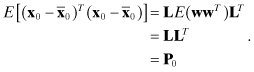
FIGURE 2.10: Simulation structure.

The initial state x0 is then
numerically integrated to the time of the first measurement where the state
differential equation is given by equation (2.2-2),![]()
if the system is nonlinear, or equation (2.2-4) if it is linear. In order to properly simulate
the effects of process noise qc(t), it may be advisable to
integrate using smaller steps than the intervals between measurements. Alternately
the discrete process noise qD(ti) could be
added after integrating ![]() , where qD(ti) is computed as qD(ti) = Lw, LLT = QD and w is a unit random vector. QD can be computed using the methods of Section
2.3.2. Then the measurement vector is computed as y(t) = h(x) and random measurement noise of specified covariance R is added. If R is nondiagonal,
Cholesky factorization should be used, as done for the initial state and process
noise. Colored noise is generated using the low-order Markov process models
discussed previously. This process is repeated through each time step of the
simulation.
, where qD(ti) is computed as qD(ti) = Lw, LLT = QD and w is a unit random vector. QD can be computed using the methods of Section
2.3.2. Then the measurement vector is computed as y(t) = h(x) and random measurement noise of specified covariance R is added. If R is nondiagonal,
Cholesky factorization should be used, as done for the initial state and process
noise. Colored noise is generated using the low-order Markov process models
discussed previously. This process is repeated through each time step of the
simulation.
2.6 COMMON MODELING ERRORS AND SYSTEM BIASES
More effort is often spent trying to determine why least-squares or Kalman estimators are not performing properly than effort spent on the initial design. The most common modeling problems are due to incorrect model structure, incorrect model parameters, incorrect process noise covariance (in Kalman filters), incorrect measurement noise covariance, or mis-modeling of system biases. Of these possibilities, mis-modeling of biases is probably the most common mistake. It is very important that potential process or measurement biases be modeled unless it is known with certainty that they are negligible.
Six examples from the author’s experience demonstrate the problem, and show that bias errors in system models are a common cause of estimation errors.
1. In 1973 the National Aeronautics and Space Administration (NASA) launched the IMP-8 spacecraft into a highly elliptical transfer orbit with an apogee altitude of about 233,000 km. At apogee, an injection motor was fired to circularize the orbit. Unfortunately, the eccentricity of the resulting orbit was 0.33 versus the target 0.096. Inclination differed from the target by about 3.4 degrees. A smaller discrepancy was also observed for the IMP-7 spacecraft. Extensive error analysis was conducted to determine the cause of the orbit error. Possibilities included errors in orbit determination, errors in determining spacecraft attitude when pointing the spacecraft for injection motor firing, and errors in the thrust vector generated by the injection motor. Analysis showed that errors in the earth and sun sensors—used for onboard spacecraft attitude determination—were the most likely cause of the problem (Gibbs and Fang 1975; Gibbs et al. 1975). It appeared that the sun sensor calibration transition points were in error by as much as 0.5 degrees and the least significant bit did not register. The earth telescope photodiode sensitivity was greater than expected and detected horizon/terminator crossings when only a small portion of the field of view was lit. This caused an earth central angle-dependent bias, which had the effect of biasing the estimated yaw and pitch. A significant sun-to-earth sensor roll bias was also present. Finally, either the spacecraft spin rate varied or the spacecraft clock drifted, causing a trend in the sensed roll. Analysis was difficult because sensitivity of spacecraft attitude to sensor biases was very high, and geometric observability of sensor biases from the available data was very weak. Also the “time-varying” earth sensor bias caused an attitude-determination Kalman filter to diverge until a correction for the telescope sensitivity error was applied. Batch least-squares attitude estimation was less affected by the earth sensor bias, but the trend in the spacecraft spin rate had to be explicitly modeled.
2. In 1974–1975 NASA and the Maritime Administration (MARAD) conducted two independent ship and aircraft navigation tests using ranging from the ground to the ATS-5 and ATS-6 geosynchronous satellites, and to ships or aircraft. Unfortunately the computed ship and aircraft positions differed by as much as 55 km from the ground truth positions, both in fixed locations and when moving. Posttest analysis revealed that the ATS-6 ephemeris—used as input to the ship/aircraft navigation algorithm—was in error by up to 11 km in longitude and 3.7 km radially. The satellite ephemeris was a prediction of the orbit determined once every 2 weeks using 1 day of ground range and range rate data. Analysis revealed that the solar radiation coefficient used in orbit determination was 50% smaller than the daily mean value, and that the area normal to the sun line varied by a factor of 3:1 during the day. Fixing these problems greatly reduced prediction errors (Gibbs 1977). Interestingly, the computed ship positions were much more sensitive to ATS-6 ephemeris errors than to ATS-5 ephemeris errors. The sensitivity reduction was due to differences in the algorithms used to preprocess the range measurements. When the MARAD algorithm was modified to process ATS-6 data similarly to ATS-5 data, the ship positions were generally accurate within 4 km even when using the erroneous ATS-6 ephemeris. No such modification was possible with the NASA algorithms used for aircraft tracking. After correcting the ephemeris, ship and aircraft positions were accurate within 4 to 7 km, but patterns in the position errors suggested that time-varying transponder biases were still a problem.
3. In a second part of the NASA/MARAD navigation test, the ATS-6 ephemeris was computed using trilateration data. The measurements available for the navigation were multi-link ranges from the ground transmitting antenna to ATS-6, to one of two ground transponders, and back along the same path. One link just involved the transmitting/receiving antenna and ATS-6. Since the range measurements were computed from phases of the four tones, it was necessary to calibrate the phase delays in the ground transponders. Unfortunately the phase delay calibration procedure used for one ground transponder was flawed, with the result that the calculated range bias was in error by 500 to 1000 m. This resulted in 1500 km crosstrack errors when using trilateration data for orbit determination.
4. During postlaunch testing of the GOES-13 geosynchronous weather satellite, it was discovered that differences between actual ground-spacecraft ranges and 1-day predictions of those ranges exhibited 10–30 m bias-ramp-sinusoidal signatures (Gibbs et al. 2008a). The pattern appeared when the spacecraft was in the “inverted” yaw orientation, but not when in the “upright” orientation. The pattern could be eliminated by adding a bias to observed range measurements, but the required bias changed with spacecraft longitude and yaw attitude, and no physical reason for that behavior was known. Even with this anomaly, GOES-13 met accuracy requirements with margin. Extensive analysis using both real and simulated data was conducted to determine whether various modeling errors could cause the signatures. It was eventually discovered that the satellite transponder delay had not been properly compensated in ground software, but this only partly explained the problem. Only one possibility was found to match observed behavior: an east-west bias between star and landmark angular measurements. Both of these measurement types are obtained from the Imager earth imaging instrument. Landmark observations are obtained when the Imager scans the earth, while star observations are obtained with fixed scan angles as the spacecraft drifts in pitch to maintain earth-nadir pointing. The exact cause of the bias is still unknown. The problem did not appear with GOES-8 to -12 spacecraft that use the same Imager design. Also, the behavior of the bias with GOES-14 (the next satellite in the NOP series) is different. It seems likely that the bias is instrument-dependent. One possibility is uncompensated fixed pattern errors in the Imager.
5. The GOES-13 ground system has the capability to calibrate spacecraft thruster magnitudes and cant angles using maneuver angular momentum (Δh) telemetry, and orbit determination solutions for maneuver velocity change (Δv). The postlaunch calibration worked successfully using data from more than 100 maneuvers, but systematic biases in Δh and Δv measurement residuals were correlated with the spacecraft configuration used for daily momentum-dumping maneuvers (Gibbs et al. May 2008b). Extensive analysis was conducted to determine the source of the biases, and this led to improvements in the thruster and plume impingement models. However, small biases still remained, and one jump in daily momentum-dumping (Δh) measurements occurred without any change in operational conditions. The source of the apparent biases is still not fully understood, but may be partly due to abrupt changes of about 2–3% in thruster performance. Imperfect alignment of the four momentum wheels with respect to spacecraft reference axes may also be a factor: the prelaunch alignment accuracy is sufficient for spacecraft attitude control purposes, but it does affect thruster calibration.
6. The onboard GOES-13 Stellar Inertial Attitude Determination utilizes three star trackers, where only two are used at any given time. The star trackers are mounted on an optical bench and aligned one time shortly after launch, but the alignment is not perfect. Even if it is, diurnal thermal deformation causes additional angular misalignments between the trackers. The onboard Kalman filter does not estimate tracker-dependent alignment biases, so the estimated spacecraft attitude varies somewhat as the filter tries to reconcile differences in measured attitude between sensors. The variation in attitude is small and does not prevent the system from meeting accuracy requirements.
It is difficult to draw general conclusions from the above examples. Most problems were caused by measurement biases, but two cases involved dynamic model biases. Some problems should have been detected before implementation, but others would have been very difficult to identify before operational data became available. Some biases only caused a minor degradation in accuracy, but the system did not meet requirements in others cases. It is concluded that
1. Incorrectly modeled biases are fairly common.
2. Every reasonable attempt should be made to identify potential sources of bias and calibrate them before operations.
3. The estimator should either estimate biases or process measurements in a manner that reduces bias effects.
4. Simulation should be used to determine sensitivity to bias errors.
2.7 SUMMARY
This chapter discussed the different types of models that may be used for least-squares or Kalman estimation. Dynamic models may be either continuous or discrete. Continuous dynamic models may be either basis function expansions in time, first-principle derivations, stochastic processes, linear regression models, or combinations of these. These models may either be parametric or nonparametric, linear or nonlinear, and time-varying or time-invariant. Stochastic models assume that the dynamic system is driven by random process noise. Stochastic models are used in Kalman filters, not least-squares estimation.
Discrete models generally assume that the process is stationary and the sampling interval is constant. Discrete models may be derived as continuous models sampled discretely, but usually the structure is defined in advance and parameters of the model are determined empirically from data. It is often assumed that measurement noise does not appear separately from process noise, but that is not a general restriction. Discrete models are often single-input/single-output, but may be multiple-input/multiple-output. Typical structures for discrete models are
1. AR: a pole-only model ideal for modeling multiple narrowband signals
2. MA: a zero-only model ideal for modeling signals with frequency nulls
3. ARMA: a pole-zero model that can handle more general signals. It is more difficult to determine the model parameters than for AR or MA
4. ARMAX: an ARMA model with exogenous (known) inputs.
Discrete models may be implemented in a variety of equivalent forms, such as the companion form (see Appendix D).
Continuous dynamic models are usually defined as a set of linear or
nonlinear first-order differential equations. If the model is nonlinear and
stochastic, the effects of process noise are usually treated as linear perturbations
of the nonlinear model. Central to both least squares and Kalman filtering is the
state transition matrix Φ. The state transition matrix
models the propagation of the state vector from one measurement time to the next in
a linear model. It is obtained by integrating the state differential equations ![]() with the result Φ(T) = eFT.
Various methods for numerically computing Φ were
discussed. Kalman filters also require the state noise covariance matrix Q. Q is defined as the expected
value of a “convolution-like” integral involving the continuous
process noise and the state transition matrix. Methods for computing Q were also discussed.
with the result Φ(T) = eFT.
Various methods for numerically computing Φ were
discussed. Kalman filters also require the state noise covariance matrix Q. Q is defined as the expected
value of a “convolution-like” integral involving the continuous
process noise and the state transition matrix. Methods for computing Q were also discussed.
Various examples showed how continuous dynamic models can be defined using basis functions, first-principle derivations, stochastic processes, linear regression structures, or combinations of these. Additional first-principle examples are presented in Chapter 3 and Appendix C. The properties of random walk and low-order Markov process models were discussed at length since they are central to most Kalman filter applications. Among other properties, it was noted that the variance of a random walk model increases with time while that of stable Markov processes is constant. Markov process models are also called colored noise models since they have a low or band-pass characteristic.
Measurements are often a direct function of dynamic model states, with added measurement noise. Measurement model examples are presented in later chapters.
The importance of simulation in design and evaluation of estimators was emphasized. Methods for simulating random initial conditions, process noise, and measurement noise were discussed. This included use of Cholesky factorization for simulating correlated noise.
Common modeling errors were discussed, and it was emphasized that the mis-modeling of system biases is probably the most common modeling error. Several examples of bias problems in operational systems were presented.
Proper design of models to be used in estimation algorithms should include the following steps.
1. Determine the requirements and goals of the estimation because this will impact the level of detail required in the design.
2. Determine if is practical to develop a first-principles model, or combined first-principles/empirical/stochastic model. This will often be the most robust approach. If this is not practical, a basis function or an empirically based model is indicated.
3. Determine which model states are important to estimation: ignore high frequency effects and unobservable linear combinations of states unless those states are important outputs. This will be discussed in greater detail later. If practical, develop several competing models and algorithms and compare performance.
4. Simulate and evaluate performance of the system, and redesign if necessary. Perform covariance or Monte Carlo simulations to verify conformance with requirements.