This Appendix summarizes properties of vector and matrices, and vector/matrix operations that are often used in estimation. Further information may be found in most books on estimation or linear algebra; for example, Golub and Van Loan (1996), DeRusso et al. (1965), and Stewart (1988).

A.1 DEFINITION

A.1.1 Vectors

A vector is a linear collection of elements. We use a lower case bold letter to denote vectors, which by default are assumed to be column vectors. For example,

is a three-element column vector. A row vector is (obviously) defined with elements in a row; for example,

A vector is called unit or normalized when the sum of elements squared is equal to 1: for an n-element vector a.

A.1.2 Matrices

A matrix is a two-dimensional collection of elements. We use bold upper case letters to denote matrices. For example,

is a matrix with two rows and three columns, or a 2 × 3 matrix. Individual elements are labeled with the first subscript indicating the row, and the second indicating the column. An n-element column vector may be considered an n × 1 matrix, and an n-element row vector may be considered a 1 × n matrix.

A.1.2.1 Symmetric Matrix

A square matrix is symmetric if elements with interchanged subscripts are equal: A_ji = A_ij. For example,

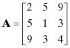
is symmetric.

A.1.2.2 Hermitian Matrix

A square complex matrix is Hermitian if elements with interchanged subscripts are equal to the complex conjugate of each other: .

A.1.2.3 Toeplitz Matrix

A square matrix is Toeplitz if all elements along the upper left to lower right diagonals are equal: A_i,j = A_i−1,j−1. For example,

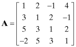
is Toeplitz.

A.1.2.4 Identity Matrix

A square matrix that is all zero except for ones along the main diagonal is the identity matrix, denoted as I. For example,

is a 4 × 4 identity matrix. Often a subscript is added to indicate the dimension, as I_n is an n × n identity matrix.

A.1.2.5 Triangular Matrix

All elements of a lower triangular matrix above the main diagonal are zero. All elements of an upper triangular matrix below the main diagonal are zero. For example,

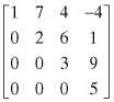
is upper triangular.

A.2 ELEMENTARY VECTOR/MATRIX OPERATIONS

A.2.1 Transpose

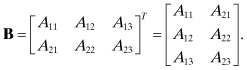
The transpose of a matrix, denoted with superscript T, is formed by interchanging row and column elements: B = A^T is the transpose of A where B_ji = A_ij. For example,

If the matrix is complex, the complex conjugate transpose is denoted as A^H = (A*)^T. The matrix is Hermitian if A = A^H.

A.2.2 Addition

Two or more vectors or matrices of the same dimensions may be added or subtracted by adding/subtracting individual elements. For example, if

then

Matrix addition is commutative; that is, C = A + B = B + A.

A.2.3 Inner (Dot) Product of Vectors

The dot product or inner product of two vectors of equal size is the sum of the products of corresponding elements. If vectors a and b both contain m elements, the dot product is a scalar:

If , the vectors are orthogonal.

A.2.4 Outer Product of Vectors

The outer product of two vectors (of possibly unequal sizes) is a matrix of products of corresponding vector elements. If vectors a and b contain m- and n-elements, respectively, then the outer product is an m × n matrix:

or C_ij = a_ib_j.

A.2.5 Multiplication

Two matrices, where the column dimension of the first (m) is equal to the row dimension of the second, may be multiplied by forming the dot product of the rows of the first matrix and the columns of the second; that is, . For example, if

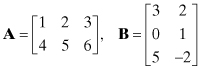
then

Matrix multiplication is not commutative; that is, C = AB ≠ BA. A matrix multiplying or multiplied by the identity I is unchanged; that is, AI = IA = A.

The transpose of the product of two matrices is the reversed product of the transposes: (AB)^T = B^TA^T.

Vector-matrix multiplication is defined as for matrix-matrix multiplication. If matrix A is m × n and vector x has m-elements, y = x^TA or

is an n-element row vector. If vector x has n elements, y = Ax is an m-element column vector.

A.3 MATRIX FUNCTIONS

A.3.1 Matrix Inverse

A square matrix that multiplies another square matrix to produce the identity matrix is called the inverse, and is denoted by a superscript −1; that is, if B = A⁻¹, then AB = BA = I. Just as scalar division by zero is not defined, a matrix is called indeterminate if the inverse does not exist. The matrix inverse may be computed by various methods. Two popular methods for general square matrices are Gauss-Jordan elimination with pivoting, and LU decomposition followed by inversion of the LU factors (see Press et al. 2007, chapter 2). Inversion based on cofactors and determinants (explained below) is also used for small matrices. For symmetric matrices, inversion based on Cholesky factorization is recommended.

The inverse of the product of two matrices is the reversed product of the inverses: (AB)⁻¹ = B⁻¹A⁻¹. Nonsquare matrices generally do not have an inverse, but left or right inverses can be defined; for example, for m × n matrix A, ((A^TA)⁻¹A^T)A = I_n, so (A^TA)⁻¹A^T is a left inverse provided that (A^TA)⁻¹ exists, and A(A^T(AA^T)⁻¹) = I_m so A^T(AA^T)⁻¹ is a right inverse provided that (AA^T)⁻¹ exists.

A square matrix is called orthogonal when A^TA = AA^T = I. Thus the transpose is also the inverse: A⁻¹ = A^T. If rectangular matrix A is m × n, it is called column orthogonal when A^TA = I since the columns are orthonormal. This is only possible when m ≥ n. If AA^T = I for m ≤ n, matrix A is called row orthogonal because the rows are orthonormal.

A square symmetric matrix must be positive definite for it to be invertible. A symmetric positive definite matrix is a square symmetric matrix for which x^TAx > 0 for all nonzero vectors x. A symmetric positive semi-definite or non-negative definite matrix is one for which x^TAx ≥ 0.

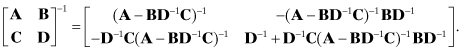
A.3.2 Partitioned Matrix Inversion

It is often helpful to compute the inverse of a matrix in partitions. For example, consider the inverse of

where the four bold letters indicate smaller matrices. We express the inverse as

and write

or

(A3-1)

(A3-2)

(A3-3)

(A3-4)

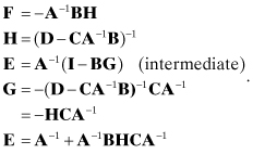
Using equations (A3-2), (A3-4), (A3-1), and (A3-3) in that order, we obtain:

(A3-5)

Alternately, using (A3-3), (A3-1), (A3-4), and (A3-2), we obtain

(A3-6)

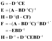
Thus the partitioned inverse can be written in two forms:

(A3-7)

or

(A3-8)

If the matrix to be inverted is symmetric:

(A3-9)

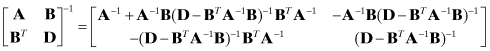
or

(A3-10)

where A and D are also symmetric.

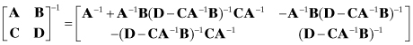
A.3.3 Matrix Inversion Identity

The two equivalent expressions for the partitioned inverse suggest a matrix equivalency that is the link between batch least squares and recursive least squares (and Kalman filtering). This formula and variations on it have been attributed to various people (e.g., Woodbury, Ho, Sherman, Morrison), but the relationship has undoubtedly been discovered and rediscovered many times.

From the lower right corner of equations (A3-7) and (A3-8):

(A3-11)

In the symmetric case when C = B^T:

(A3-12)

or by changing the sign of A:

(A3-13)

Equation (A3-13) is the connection between the measurement update of Bayesian least squares and the Kalman filter.

If D = I and C = B^T:

(A3-14)

or

(A3-15)

If b is a row vector and a is scalar:

(A3-16)

or

(A3-17)

A.3.4 Determinant

The determinant of a square matrix is a measure of scale change when the matrix is viewed as a linear transformation. When the determinant of a matrix is zero, the matrix is indeterminate or singular, and cannot be inverted. The rank of matrix |A| is the largest square array in A that has nonzero determinant.

The determinant of matrix A is denoted as det(A) or |A|. Laplace’s method for computing determinants uses cofactors, where a cofactor of a given matrix element ij is C_ij = (−1)^i+j|M_ij| and M_ij, called the minor of ij, is the matrix formed by deleting the i row and j column of matrix A. For 2 × 2 matrix

the cofactors are

The determinant is the sum of the products of matrix elements and cofactors for any row or column. Thus

For a 3 × 3 matrix A,

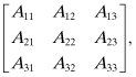
the cofactors are

so using the first column,

A matrix inverse can be computed from the determinant and cofactors as

(A3-18)

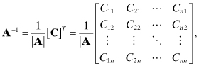
where [C] is the matrix of cofactors for A.

Computation of determinants using cofactors is cumbersome, and is seldom used for dimensions greater than three. The determinant is more easily computed by factoring A = LU using Crout reduction, where L is unit lower triangular and U is upper triangular. Since the determinant of the product of matrices is equal to the product of determinants,

(A3-19)

we have |A| = |L||U|, which is simply equal to the product of the diagonals of U because |L| = 1. A number of other methods may also be used to compute determinants. Often the determinant is a bi-product of matrix inversion algorithms.

A.3.5 Matrix Trace

The trace of a square matrix is the sum of the diagonal elements. This property is often useful in least-squares or minimum variance estimation, as the sum of squared elements in an n-vector can be written as

(A3-20)

This rearrangement of vector order often allows solutions for minimum variance problems: it has been used repeatedly in previous chapters.

Since the trace only involves diagonal elements, tr(A^T) = tr(A). Also,

(A3-21)

and for scalar c,

(A3-22)

Unlike the determinant, the trace of the matrix products is not the product of traces. If A is an n × m matrix and B is an m × n matrix,

(A3-23)

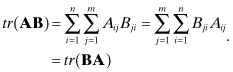
However, this commutative property only works for pairs of matrices, or interchange of “halves” of the matrix product:

(A3-24)

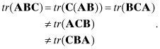
When the three individual matrices are square and symmetric, any permutation works:

(A3-25)

This permutation does not work with four or more symmetric matrices.

Permutation can be used to express the weighted quadratic form a^TWa as

(A3-26)

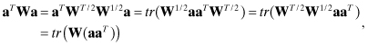
where a is a vector and matrix W = W^T/2W^1/2 is symmetric.

For a transformation of the form T⁻¹AT (called a similarity transformation), the trace is unchanged:

(A3-27)

A.3.6 Derivatives of Matrix Functions

The derivative of matrix A with respect to scalar variable t is ∂A/∂t, which is a matrix with the same dimensions as A. The derivative of matrix product BA with respect to t can be written as

(A3-28)

where ∂(BA)/∂A is a four-dimensional variable:

Thus matrix derivatives for a function of A, C(A), can be written using ∂C/∂A if the four dimensions are properly handled.

The derivative of the inverse of a matrix is obtained by differentiating AB = I, which gives (dA)B + A(dB) = 0. Thus

is two-dimensional, but has perturbations with respect to all elements of dA; that is, each i, j element (dB)_ij is a matrix of derivatives for all perturbations dA. Thus

(A3-29)

The derivative of the trace of matrix products is computed by examining the derivative with respect to an individual element:

Thus

(A3-30)

For products of three matrices,

(A3-31)

The derivative of the determinant is computed by rearranging equation (A3-18) as

(A3-32)

Thus for any diagonal element i = 1, 2,…, n,

The partial derivative of |A| with respect to any A element in row i is

where ∂C_ik/∂A_ij = 0 from cofactor definitions. Hence

(A3-33)

By a similar development

(A3-34)

A.3.7 Norms

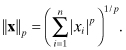
Norm of vectors or matrices is often useful when analyzing growth of numerical errors. The Hölder p-norms for vectors are defined as

(A3-35)

The most frequently used p-norms are

(A3-36)

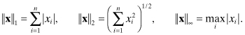
The l₂-norm x₂ is also called the Euclidian or root-sum-squared norm.

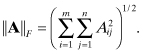
An l₂-like norm can be defined for matrices by treating the matrix elements as a vector. This leads to the Frobenius norm

(A3-37)

Induced matrix norms measure the ability of matrix A to modify the magnitude of a vector; that is,

The l₁-norm is where a_:j is the j-th column of A, and the l_∞-norm is where a_i: is the i-th row of A. It is more difficult to compute an l₂-norm based on this definition than a Frobenius norm. A₂ is equal to the square root of the maximum eigenvalue of A^TA—or equivalently the largest singular value of A. These terms are defined in Section A.4.

Norms of matrix products obey inequality conditions:

(A3-38)

The l₂ and Frobenius matrix norms are unchanged by orthogonal transformations, that is,

(A3-39)

A.4 MATRIX TRANSFORMATIONS AND FACTORIZATION

A.4.1 LU Decomposition

LU decomposition has been mentioned previously. Crout reduction is used to factor square matrix A = LU where L is unit lower triangular and U is upper triangular. This is often used for matrix inversion or when repeatedly solving equations of the form Ax = y for x. The equation Lz = y is first solved for z using forward substitution, and then Ux = z is solved for x using backward substitution.

A.4.2 Cholesky Factorization

Cholesky factorization is essentially LU decomposition for symmetric matrices. Usually it implies A = LL^T where L is lower triangular, but it is sometimes used to indicate A = L^TL. Cholesky factorization for symmetric matrices is much more efficient and accurate than LU decomposition.

A.4.3 Similarity Transformation

A similarity transformation on square matrix A is one of the form B = T⁻¹AT. Since TB = AT, matrices A and B are called similar. Similarity transformations can be used to reduce a given matrix to an equivalent canonical form; for example, eigen decomposition and singular value decomposition discussed below.

A.4.4 Eigen Decomposition

The vectors x_i for which Ax_i = λ_ix_i, where λ_i are scalars, are called the eigenvectors of square matrix A. For an n × n matrix A, there will be n eigenvectors x_i with corresponding eigenvalues λ_i. The λ_i may be complex (occurring in complex conjugate pairs) even when A is real, and some eigenvalues may be repeated. The eigenvectors are the directions that are invariant with pre-multiplication by A.

The eigenvector/eigenvalue relationship can be written in matrix form as

(A4-1)

or

(A4-2)

where

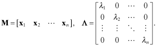
Matrix M is called the modal matrix and λ_i are the eigenvalues. The eigenvalues are the roots of the characteristic polynomial p(s) = |sI − A|, and they define the spectral response of the linear system when x(t) is the system state vector (not eigenvectors). Eigen decomposition is a similarity transformation, and thus

(A4-3)

Also

(A4-4)

When real A is symmetric and nonsingular, the λ_i are all real, and the eigenvectors are distinct and orthogonal. Thus M⁻¹ = M^T and A = MΛM^T.

Eigenvectors and eigenvalues are computed in LAPACK using either generalized QR decomposition or a divide-and-conquer approach.

A.4.5 Singular Value Decomposition (SVD)

While eigen decomposition is used for square matrices, SVD is used for either square or rectangular matrices. The SVD of m × n matrix A is

(A4-5)

where U is an m × m orthogonal matrix (UU^T = I_m), V is an n × n orthogonal matrix (VV^T = I_n), and S is an m × n upper diagonal matrix of singular values. In least-squares problems m > n is typical, so

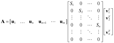
where u_i are the left singular vectors and v_i are the right singular vectors. The left singular vectors u_n+1, u_n+2,…, u_m are the nullspace of A as they multiply zeroes in S. The above SVD is called “full,” but some SVD utilities have the option to omit computation of u_n+1, u_n+2,…, u_m. These are called “thin” SVDs.

When A is a real symmetric matrix formed as A = H^TH (such as the information matrix in least-squares estimation), the eigenvalues of A are the squares of the singular values of H, and the eigenvectors are the right singular vectors v_i. This is seen from

The accuracy of the SVD factorization is much greater than that for eigen decomposition of A = H^TH because the “squaring” operation doubles the condition number (defined below). This doubles sensitivity to numerical round-off errors.

A.4.6 Pseudo-Inverse

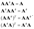
When A is rectangular or singular, A does not have an inverse. However, Penrose (1955) defined a pseudo-inverse A^# uniquely determined by four properties:

(A4-6)

This Moore-Penrose pseudo-inverse is sometimes used in least-squares problems when there is insufficient measurement information to obtain a unique solution. A pseudo-inverse for the least-squares problem based on measurement equation y = Hx + r can be written using the SVD of H = USV^T. Then the normal equation least-squares solution is obtained using the pseudo-inverse of H,

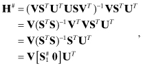
where is the pseudo-inverse of the nonzero square portion of S. For singular values that are exactly zero, they are replaced with zero in the same location when forming . Thus

This shows that a pseudo-inverse can be computed even when H^TH is singular. The pseudo-inverse provides the minimal norm solution for a rank-deficient (rank < min(m,n)) H matrix.

A.4.7 Condition Number

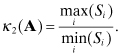
The condition number of square matrix A is a measure of sensitivity of errors in A⁻¹ to perturbations in A. This is used to analyze growth of numerical errors. The condition number is denoted as

(A4-7)

when using the an l_p induced matrix norm for A. Because it is generally not convenient to compute condition numbers by inverting a matrix, they are most often computed from the singular values of matrix A. Decomposing A = USV^T where U and V are orthogonal and S_i are the singular values in S, then

(A4-8)