
CHAPTER 9
FILTERING FOR NONLINEAR SYSTEMS, SMOOTHING, ERROR ANALYSIS/MODEL DESIGN, AND MEASUREMENT PREPROCESSING
This chapter covers extensions of Kalman filtering that are routinely used. Specific topics considered in this chapter are:
1. Kalman filtering for nonlinear systems: The standard techniques include linearization about a reference trajectory (linearized filtering), linearization about the current estimate (extended Kalman filtering), and iterated linearized filtering (iterated extended Kalman filter or iterated linear filter-smoother). The extended Kalman filter is probably the most frequently used Kalman filter implementation.
2. Smoothing: Smoothers compute the minimum mean-squared error (MMSE) estimate of a state in past time based on measurements up to a later time. Smoothing options include fixed point, fixed lag, and fixed interval.
3. Error analysis and model state selection: Error analysis should be a necessary step in most Kalman filter implementations. As with least-squares estimation, Monte Carlo and covariance error analysis can be used. Options for linear covariance error analysis include perturbation analysis of independent error sources (measurement noise, process noise, and errors in unadjusted or “considered” model parameters), error analysis for reduced-order models (ROMs) defined as transformations on detailed models, and error analysis for truth and filter models that are structurally different but a subset of important states are common to both. Analysis of different model structures is important when attempting to develop a high-accuracy filter that is insensitive to model structure and parameter assumptions.
4. Measurement preprocessing: A Kalman filter that has reached steady-state conditions can be very effective in identifying anomalous measurements. During the initialization period, however, it is much less effective. Because the filter has an infinite impulse response (IIR) characteristic, it is important that anomalous measurements be edited during preprocessing. The available preprocessing methods are essentially the same as described for least-squares estimation.
9.1 NONLINEAR FILTERING
Although Kalman’s original (1960) paper used linear models, the first application was for a nonlinear system: navigation of the Apollo spacecraft. As described by McGee and Schmidt (1985), Stanley Schmidt worked in the Dynamics Analysis Branch at Ames Research Center, and in 1960 that group had the task of designing the midcourse navigation and guidance for the Apollo circumlunar mission. It was assumed that the spacecraft crew would use an inertially referenced optical sensor to measure angles to the earth and moon. However, the method of computing the navigation solution was unclear. Iterative weighted least squares was too complex for state-of-the-art onboard computers. Wiener filtering could not be applied without making approximations that would restrict the observation system or degrade accuracy. Other alternatives could not meet accuracy requirements.
Fortunately Kalman visited Ames in the fall of 1960, and the staff immediately recognized the usefulness of Kalman’s sequential solution. However, it was not at first clear how the linear filter would be used for the nonlinear system. Partly because the Ames staff had already been using linear perturbation concepts in guidance studies, Schmidt realized that the nonlinear trajectory equations could be linearized about a reference trajectory if the filter equations were broken into separate discrete time and measurement updates. It was also suspected that better results would be obtained if the linearization was recomputed using the current state solution at each step. Although many details and practical problems remained, the approach allowed successful navigation to the moon. Because of this experience and others, Schmidt enthusiastically promoted use of Kalman’s filter.
Schmidt’s modification was at first called the Kalman-Schmidt filter by some authors, but it came to be accepted as the extended Kalman filter (EKF). Because the vast majority of applications are for nonlinear systems, it is often just called the Kalman filter.
9.1.1 Linearized and Extended Kalman Filters
The extended Kalman filter (EKF) assumes that the nonlinear system dynamic and measurement models can be expanded in first-order Taylor series about the current estimate. That is, the filter time update becomes
(9.1-1)
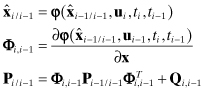
where ![]() is usually obtained by numerically integrating the state differential equation
is usually obtained by numerically integrating the state differential equation ![]() as described in Section 2.2, and we again use the simplified notation
as described in Section 2.2, and we again use the simplified notation
![]()
The state noise covariance Qi,j−1 is also obtained using the methods of Section 2.2.1.
The EKF measurement update is then
(9.1-2)
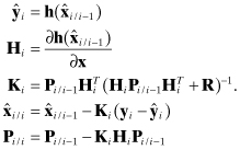
The Joseph form of the Pi/i update can also be used.
Early users of the EKF reported that filters sometimes became unresponsive to measurements and/or the state estimate diverged from true values much more than predicted by the filter covariance matrix. These problems were often caused by modeling errors, outlying measurements, or numerical instability resulting from single precision implementations and/or failure to keep Pi/i symmetric. The divergence problem is more serious in an extended filter than a linear filter because partial derivatives are evaluated at the current state estimate, and if that deviates from truth, partials will be incorrect causing further divergence.
For some applications in which the process and measurement noise is small and models are good, an accurate reference trajectory can be computed prior to filtering. Then the filter partial derivatives Φi,i−1 and Hi are evaluated along the reference trajectory. Satellite orbit determination for mid and high earth orbit spacecraft is one example where a limited tracking span allows fairly accurate ephemeris predictions for periods of days. For low altitude satellites, batch least-squares solutions can be used as a reference trajectory for a Kalman filter/smoother that improves the accuracy of the orbit (Gibbs 1978, 1979). Use of an accurate reference trajectory may help avoid accelerated divergence due to incorrect partials, although it does not alleviate effects of measurement outlier, modeling, or numerical errors. The linearized Kalman filter is nearly identical to an extended filter but Φi,i−1 and Hi are computed as
(9.1-3)
![]()
and
(9.1-4)
![]()
where ![]() is the reference trajectory.
is the reference trajectory.
Most Kalman filter applications involve nonlinear systems and use the EKF described above. The EKF would not be so widely accepted if the approach was not successful. However, our first example is intended to make you cautious when working with nonlinear systems. Later examples show more positive results.
Example 9.1: Nonlinear Measurement Model for Bias State
A trivial one-state, one-measurement model demonstrates some of the problems encountered when working with nonlinear models and the EKF. This example uses a bias state x with a scalar measurement that is a nonlinear function of the state:
![]()
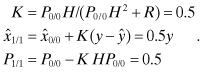
where E[r] = 0, R = E[r2] = 1 and x = 0. To make the effect of the nonlinearity significant, we set α = 0.5. The a priori filter estimate is ![]() (optimistically equal to the true value) and
(optimistically equal to the true value) and ![]() . The EKF model of the measurement and partial derivative is
. The EKF model of the measurement and partial derivative is
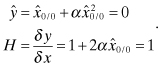
Since x is a bias, the time update is simply ![]() and P1/0 = P0/0. Using the above values, the Kalman gain, a posteriori state estimate and covariance are computed as
and P1/0 = P0/0. Using the above values, the Kalman gain, a posteriori state estimate and covariance are computed as
Now we consider the problem using probability density functions. Recall from Chapter 4 that the minimum variance/MMSE estimate for linear or nonlinear models is the conditional mean; that is, the mean x of the density function
![]()
where pY|X(y|x) is the conditional probability density of receiving the measurement given the state x, pX(x) is the prior density function of x, and
![]()
Assuming that the one-dimensional distributions are Gaussian,
![]()
and
![]()
for the measurement model y = h(x) + r. The conditional mean is computed as
![]()
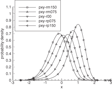
Figure 9.1 shows pX|Y(x|y) for the given example model with y computed using different values of the measurement noise r. The lines are labeled as
![]()
![]()
![]()
![]()
![]()
FIGURE 9.1: Conditional probability density for one-state model with filter x0 = 0.

The largest r value is only 1.5 times the specified noise standard deviation, so these are typical noise magnitudes. Notice that the conditional distributions are highly skewed for all cases (even r = 0). Table 9.1 lists the mean and mode of pX|Y(x|y) and the EKF estimate. Notice that the EKF estimate does not match either the mean or the mode, but it is closer to the mode for all cases except r = −1.5. Neither the conditional mean nor the mode are symmetric about r = 0, but the mode is closer to symmetric. The EKF estimate is symmetric about r = 0 because ![]() when
when ![]() . As expected, the root-mean-squared (RMS) error from the true x = 0 is slightly smaller for the conditional mean estimate (0.412) than for the conditional mode (0.475) or the EKF (0.530). (Note: The nonlinear equations for
. As expected, the root-mean-squared (RMS) error from the true x = 0 is slightly smaller for the conditional mean estimate (0.412) than for the conditional mode (0.475) or the EKF (0.530). (Note: The nonlinear equations for ![]() and H can be substituted in equation (4.4-21) to compute Maximum A Posteriori (MAP) solutions for x. Those agree with the mode pX|Y(x|y) values listed in Table 9.1.)
and H can be substituted in equation (4.4-21) to compute Maximum A Posteriori (MAP) solutions for x. Those agree with the mode pX|Y(x|y) values listed in Table 9.1.)
TABLE 9.1: State Estimates for One-State Model with Filter x0 = 0

Figure 9.2 and Table 9.2 show the results when ![]() rather than the true value (x = 0). Again the conditional distributions are highly skewed and the EKF estimate is closer to the mode than the mean. In this case the RMS error of the conditional mean is larger than either the conditional mode or the EKF estimate. However, Monte Carlo simulation using random samples of the true x distributed as
rather than the true value (x = 0). Again the conditional distributions are highly skewed and the EKF estimate is closer to the mode than the mean. In this case the RMS error of the conditional mean is larger than either the conditional mode or the EKF estimate. However, Monte Carlo simulation using random samples of the true x distributed as ![]() shows that the RMS error of the conditional mean is about 4–7% smaller than either the mode or the EKF estimates, which supports the assertion that the conditional mean is the minimum variance estimate. In fact, the conditional mean is essentially unbiased, while the mode and EKF estimates have a significant bias error (∼0.23).
shows that the RMS error of the conditional mean is about 4–7% smaller than either the mode or the EKF estimates, which supports the assertion that the conditional mean is the minimum variance estimate. In fact, the conditional mean is essentially unbiased, while the mode and EKF estimates have a significant bias error (∼0.23).
TABLE 9.2: State Estimates for One-State Model with Filter x0 = 1
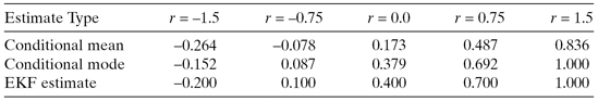
FIGURE 9.2: Conditional probability density for one-state model with filter x0 = 1.
The bias in EKF or conditional mode estimates is a function of the magnitude of the nonlinearity compared with the measurement noise. When the effect of the nonlinearity for expected variations in state estimates is small compared with the measurement noise standard deviation, the EKF estimate should be reasonably accurate and unbiased. More precisely, for a Taylor series expansion of the measurement model about the current state estimate,
![]()
the effect of the quadratic and higher order terms for the given state uncertainty specified by Px should be small compared with the specified measurement noise; that is,
![]()
where ![]() . This relationship should apply for every processed measurement. In the current example, when
. This relationship should apply for every processed measurement. In the current example, when ![]() rather than 1, the conditional mean, mode, and EKF estimates are all nearly unbiased and match within a few percent.
rather than 1, the conditional mean, mode, and EKF estimates are all nearly unbiased and match within a few percent.
To summarize, when nonlinearities for the expected error in state estimates are significant relative to measurement noise, the EKF estimate will be biased and the computed error covariance will underestimate actual errors. In some cases the bias can cause the filter to diverge from the true state. The EKF estimate for each measurement is not minimum variance. However, because the EKF is a feedback loop, it will usually (but not always) converge to the correct answer after processing many measurements, even if convergence takes longer than it should. In this particular example, the bias in the EKF estimate decayed at about the same rate as the uncertainty computed from the a posteriori covariance, and the behavior was not significantly different from that of the linear case with α = 0. Figure 9.3 shows the state estimate (“xf”) and 1 − σ uncertainty (“sig_xf”) for one Monte Carlo sample using 10,000 measurements.
FIGURE 9.3: EKF estimate and uncertainty for one-state model.

9.1.2 Iterated Extended Kalman Filter
The EKF problems of bias and divergence were noticed within the first few years after Kalman and Schmidt introduced the technique. Hence alternate methods for handling nonlinearities were developed. Some approaches include higher order terms in the filter design, but these require higher order partial derivatives and they are generally difficult to compute and implement. Jazwinski (1970) summarizes early research in these areas, and compares second-order filters with two approaches that are fairly easy to implement: the iterated extended Kalman filter (IEKF) and the iterated linear filter-smoother. Gelb (1974, sections 6.1 and 6.2) compares the iterated filter with higher order filters and a statistically linearized filter that characterizes the nonlinearity using describing functions.
The IEKF was apparently developed by J. Breakwell, and then analyzed by Denham and Pines (1966). The a posteriori state estimate obtained after processing a measurement is used in the IEKF as the reference state for recomputing Hi. In the iterated linear filter-smoother due to Wishner et al. (1968), the a posteriori state estimate is used to recompute both Φi,i−1 and Hi. That is, the time and measurement updates are recomputed using the new Φi,i−1 and Hi, and this is repeated until the change in state estimates is small. Both algorithms are implemented to avoid weighting the measurements in the solution more than once.
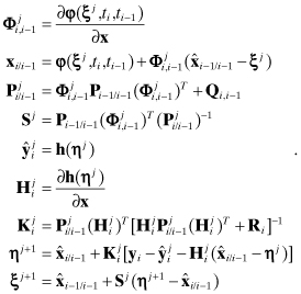
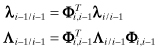
For the IEKF, the following measurement update equations are repeated:
(9.1-5)

(In these equations the superscript j is the iteration counter, not an exponent.) The iterations are initialized with ![]() . When converged, the updated state for the final iteration j is set as
. When converged, the updated state for the final iteration j is set as ![]() , and the covariance is computed as
, and the covariance is computed as
![]()
or using the Joseph form.
The IEKF only attempts to remove the effects of measurement model nonlinearities. The iterated linear filter-smoother improves both the measurement and dynamic model reference trajectory when computing partial derivatives. Because the method requires modifying ![]() after updating
after updating ![]() , the smoothing iterations are more complicated. The iterations are initialized with
, the smoothing iterations are more complicated. The iterations are initialized with ![]() and
and ![]() for the state dynamic model
for the state dynamic model ![]() . Then the following equations are repeated in the order shown until changes in ηj are negligible:
. Then the following equations are repeated in the order shown until changes in ηj are negligible:
(9.1-6)
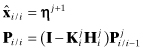
After convergence compute
(9.1-7)
The Joseph form of the covariance update can also be used. Jazwinski (1970, chapter 9) shows that the IEKF solution is always equal to the mode of the conditional density. Hence while an IEKF solution may be more accurate than an EKF solution, it is not minimum variance and does not eliminate the estimate bias. Depending upon the type of nonlinearity, the iterations are not guaranteed to converge. However, the methods are easy to implement and are computationally efficient. The statistically linearized filter (Gelb 1974, section 6.2) is slightly more difficult to implement and possibly slower than the iterated filters, but may be useful for some problems. Newer techniques that evaluate the nonlinear equations at selected points (allowing computation of first- and second-order moments) are discussed in Chapter 11.
Example 9.2: Continuation of Example 9.1 Using the IEKF
Example 9.1 did not include a time update model because the state is a bias. Hence we use the IEKF rather than the iterated filter-smoother for this example. In each case the IEKF solutions are identical to the conditional mode values of Tables 9.1 and 9.2, which are slightly different from the EKF solutions. However, the number of iterations required for state convergence within 0.001 varies greatly. With r = −1.5 and ![]() , the iterations are barely stable (62 iterations are required), which is a reason for caution when using this method. For r = 0 to 1.5, only two to three iterations are required.
, the iterations are barely stable (62 iterations are required), which is a reason for caution when using this method. For r = 0 to 1.5, only two to three iterations are required.
Using a scalar example with quadratic dynamic and cubic measurement model nonlinearities, Jazwinski shows that IEKF solutions closely match both the mean of the conditional probability density and estimates obtained using a modified Gaussian second-order filter. The EKF estimates are biased, although they eventually converge to the true state. Jazwinski’s result may or may not be more representative of typical real applications than our bias example. Gelb (1974, example 6.1-3) shows that the IEKF is more accurate than either the EKF or a second-order filter for range tracking of a falling ball—similar to our Example 7.3 but with an unknown atmospheric drag coefficient. Gelb also shows that the statistically linearized filter is superior to the EKF or higher order filters for a scalar nonlinear measurement problem, but the iterated filters were not tested for this example. Wishner et al. (1969) show that iterated filters can reduce estimation errors compared with the EKF.
It is surprisingly difficult to find real-world problems for which the performance of the iterated filters is superior to that of the EKF. This statement is generally true for most approaches to nonlinear filtering. For mildly nonlinear problems the EKF works well and iterated (or other nonlinear filters) do not improve the solution significantly. For more significant nonlinearities, the iterated filters sometimes fail to converge in cases when the EKF provides a satisfactory (if not optimal) solution. There are some problems for which the iterated filters work better than the EKF, but general characteristics of these problems are not clear.
We compared the EKF with iterated filters for the passive ship tracking problem of Section 3.1 (also used as Example 7.4), and the maneuvering tank and aircraft problems of Section 3.2. Unfortunately the poor observability and nonlinearity of the ship passive tracking problem does not allow any recursive filter method making only one pass through the measurements to be competitive with Gauss-Newton iterations that re-linearize about the current trajectory at each iteration. To make the problem more suitable for the EKF, the measurement sampling rate was increased, measurement accuracy was improved, and the initial state covariance was set to a smaller value than that of Example 7.4. Even so, the IEKF often failed to converge (usually with very erratic steps) in cases where the EKF worked satisfactorily. For the tank tracking problem with measurement sampling intervals of 0.1, and the aircraft tracking problem with 1 s measurement sampling, the performance of the EKF and iterated filter-smoother was essentially the same. Results for the tank and aircraft tracking problems are shown in Section 9.2 when discussing smoothing.
As stated at the beginning of this book, you should evaluate different algorithms for your particular application because results obtained for simple examples do not necessarily apply to other problems.
9.2 SMOOTHING
As explained in Chapter 1, Kalman and Wiener filters can be used to not only provide the optimal estimate of the system state at the time of the last measurement, but also to compute the optimal estimate at future or past times. When modeling errors do not exist, the optimum linear predictor is obtained by simply the integrating the filter state to the time of interest. However, when the system under consideration is stochastic (subject to random perturbations), the effect of process noise must be accounted for when computing optimal smoothed state estimates for times in the past. The smoothing operation effectively gives more weight to measurements near the time of the smoothed estimates than those further away. Smoothed estimates are computed using a time history of filter estimates, or information that is equivalent.
Since smoothing requires significant computation and coding effort, you may wonder if it necessary to compute a smoothed estimate rather than simply using the filtered state at the desired time. Smoothed estimates are usually much more accurate than filtered estimates because both past and future measurements are used to compute the smoothed estimate at each time point. In some cases smoothing will also average the effects of modeling errors, thus further improving the estimate.
There are three general categories of smoothing:
1. Fixed point: the smoothed state is only computed at a fixed point in time, or possibly several fixed points. This can be implemented as a real-time processor.
2. Fixed lag: the smoothed state is computed at a fixed lag in time from the current measurement; that is, the smoothed epoch moves as new measurements become available. The smoothed epoch must match a measurement time. This can also be implemented for real-time processing.
3. Fixed interval: smoothed state estimates are computed at every measurement time from the start to the end. Fixed-interval smoothing is generally only used for post-processing since all the data must be available.
We now consider each of these cases. Although both continuous-time and discrete-time smoothing algorithms exist, we only describe the discrete-time versions since these are the primary methods implemented. The continuous-time versions are more useful when analyzing smoother behavior, and when deriving other algorithms.
9.2.1 Fixed-Point Smoother
Equations defining the fixed-point smoother may be found in many references (e.g., Gelb 1974; Maybeck 1982a; Simon 2006), but it is often easier to augment the filter state with a copy of the current state at the desired smoothing time. This can be repeated multiple times to obtain multiple fixed-point smoothed estimates.
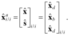
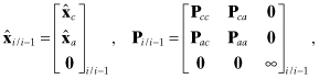
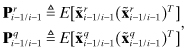
Mathematically this is implemented as follows. Let ![]() be the a posteriori filter state n-vector at time ti, and Pxx_i/i be the corresponding n × n error covariance matrix. Time ti is a desired point at which a smoothed estimate is required. We assume that the state is composed of nd dynamic and nb bias states:
be the a posteriori filter state n-vector at time ti, and Pxx_i/i be the corresponding n × n error covariance matrix. Time ti is a desired point at which a smoothed estimate is required. We assume that the state is composed of nd dynamic and nb bias states:
(9.2-1)
![]()
with associated covariance
(9.2-2)
![]()
expressed in partitions of dynamic and bias states. Since bias states are not driven by process noise and are not smoothable, it is not necessary to include them as smoothed states. We define the smoothed estimate of the dynamic states at time ti based on measurements up to and including tj (where j ≥ i) as
(9.2-3)
![]()
It is not necessary for ![]() to include all nd states, but for this discussion we assume that it does. After processing measurements at the desired smoothing time ti, an augmented state vector of dimension 2nd + nb is created by appending
to include all nd states, but for this discussion we assume that it does. After processing measurements at the desired smoothing time ti, an augmented state vector of dimension 2nd + nb is created by appending ![]() to the bottom of the filter state vector:
to the bottom of the filter state vector:
(9.2-4)
Notice that the smoothed state ![]() is initialized with a copy of
is initialized with a copy of ![]() . The error covariance is likewise augmented and initialized as
. The error covariance is likewise augmented and initialized as
(9.2-5)
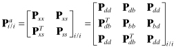
where ![]() and
and ![]() are initialized as
are initialized as
(9.2-6)
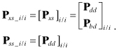
Notice that the covariance ![]() is singular at this point, but that has no impact on subsequent processing. Since the added “smoothed” states are effectively biases, they can be handled as other biases, but the smoothed states do not appear in either the dynamic or measurement models. As future measurements are processed, the smoothed states
is singular at this point, but that has no impact on subsequent processing. Since the added “smoothed” states are effectively biases, they can be handled as other biases, but the smoothed states do not appear in either the dynamic or measurement models. As future measurements are processed, the smoothed states ![]() for j > i are automatically updated because the covariance term Pxs_i/j couples changes in
for j > i are automatically updated because the covariance term Pxs_i/j couples changes in ![]() to
to ![]() .
.
The state transition matrix for the next measurement time becomes
(9.2-7)
![]()
and the state process noise matrix is
(9.2-8)
![]()
where
![]()
are the state transition and process noise matrices for the original n-state system ![]() . The augmented measurement sensitivity matrix is equal to the original H matrix with nd added zero columns:
. The augmented measurement sensitivity matrix is equal to the original H matrix with nd added zero columns:
(9.2-9)
![]()
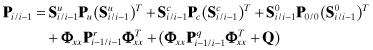
Provided that the filter is implemented to handle bias states efficiently (avoiding multiplications by 0 or 1 and taking advantage of symmetry), this implementation of the fixed-point smoother requires approximately the same number of floating point operations as explicit implementation of the fixed-point smoothing equations, but it is easier to implement. It also has the advantage that general-purpose Kalman filter libraries can be used.
It is not difficult, however, to express the time and measurement update for the separate partitions using the above matrix equations. The time update is
(9.2-10)
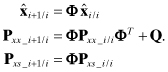
Notice that time updates are not required for ![]() and Pss, and the multiplication ΦPxs_i/i is the only extra calculation required beyond the normal filter time update. The measurement update is
and Pss, and the multiplication ΦPxs_i/i is the only extra calculation required beyond the normal filter time update. The measurement update is
(9.2-11)
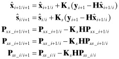
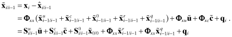
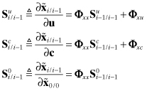
for gain matrices
(9.2-12)
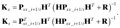
The equations for Kx, ![]() , and Pxx are the normal filter measurement update. As with all Kalman filter implementations, the covariances Pxx and Pss should be forced to be symmetric. We have expressed the state update using linear operations, but the nonlinear form of the EKF may also be used. As expected, neither the smoothed state nor the smoothed covariance affect the original filter state
, and Pxx are the normal filter measurement update. As with all Kalman filter implementations, the covariances Pxx and Pss should be forced to be symmetric. We have expressed the state update using linear operations, but the nonlinear form of the EKF may also be used. As expected, neither the smoothed state nor the smoothed covariance affect the original filter state ![]() . Calculation of smoothed states requires additional computations but does not alter the original filter equations for
. Calculation of smoothed states requires additional computations but does not alter the original filter equations for ![]() and Pxx. As before, significant computational savings are possible by storing intermediate products, although that may not be important unless the state size is large.
and Pxx. As before, significant computational savings are possible by storing intermediate products, although that may not be important unless the state size is large.
Notice that gain equation for the smoothed state can also be written as
(9.2-13)
![]()
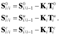
This suggests the fixed-point smoother equations can be written in other forms that do not require separate calculation of Pxs and Pss. The equations for the full state vector (including nonsmoothable biases) are

for j > i where
is initialized with Bi = I, and recursively updated. This form of the fixed-point smoother requires the same storage as the previous equations—the upper nd rows of Bj are the same size as Pxs plus Pss. However, equation (9.2-15) requires inversion of the (nd + nb) × (nd + nb) symmetric matrix Pxx_j/j−1 and several other matrix products that involve at least nd(nd + nb)2 multiplications. Since equations (9.2-14) and (9.2-15) do not reduce storage or computations and it is usually easier to implement the smoother by augmenting the state at the desired smoothing point, this form is infrequently used.
9.2.2 Fixed-Lag Smoother
The augmented state fixed-point smoother method above can be used to implement a fixed-lag smoother when the number of lags is small. For example, if the smoothing lag corresponds to three measurement time intervals, the augmented a posteriori state vector at ti is defined as

Before processing the time update of the next measurement, the elements of ![]() corresponding to
corresponding to ![]() are replaced with
are replaced with ![]() and the original
and the original ![]() elements are replaced with
elements are replaced with ![]() . Finally the
. Finally the ![]() elements are replaced with the dynamic states
elements are replaced with the dynamic states ![]() . Hence the a priori state vector used to process the next measurement becomes
. Hence the a priori state vector used to process the next measurement becomes

where ![]() . The corresponding elements of the covariance must also be shifted and the new covariance terms set as Pss_i/i = Pdd_i/i and Pds_i/i = Pdd_i/i. This process of shifting and replacing is repeated at every measurement time. When the desired smoothing lag is significant, this results in a large state vector and covariance with consequent impact on the computational burden. However, it is relatively easy to implement using standard filter software.
. The corresponding elements of the covariance must also be shifted and the new covariance terms set as Pss_i/i = Pdd_i/i and Pds_i/i = Pdd_i/i. This process of shifting and replacing is repeated at every measurement time. When the desired smoothing lag is significant, this results in a large state vector and covariance with consequent impact on the computational burden. However, it is relatively easy to implement using standard filter software.
One form of the discrete-time fixed-lag smoother appears in Gelb (1974, section 5.4) and Maybeck (1982a, section 8.6). It uses the full state vector rather than just dynamic states. Denoting N as the smoothing lag, the equations are:
(9.2-16)

where
(9.2-17)

All other variables are the output of the normal Kalman filter. The smoothed estimate and covariance are initialized with ![]() and P0/N obtained from observation time N of a fixed-point smoother. Notice that this version also requires that arrays (Ai) be stored over the smoothing lag interval, with a new array added and an old one dropped from storage at each measurement step. A matrix inversion is also required. Simon (2006, section 9.3) presents a different form of the smoother that does not require matrix inversion.
and P0/N obtained from observation time N of a fixed-point smoother. Notice that this version also requires that arrays (Ai) be stored over the smoothing lag interval, with a new array added and an old one dropped from storage at each measurement step. A matrix inversion is also required. Simon (2006, section 9.3) presents a different form of the smoother that does not require matrix inversion.
9.2.3 Fixed-Interval Smoother
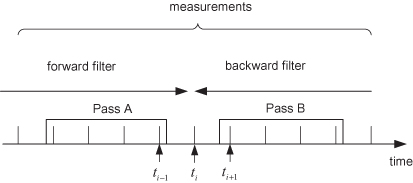
While the fixed-point and fixed-lag smoothers can be used for real-time processing, the fixed interval smoother is used after all measurements have been processed by the filter. Fraser and Potter (1969) describe the optimal linear smoother as a combination of an optimal filter operating forward in time and another filter operating backward in time, as shown in Figure 9.4.
FIGURE 9.4: Fixed-interval smoother as combination of forward and backward filters.
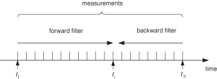
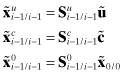
Since the measurement and process noises used in the two filters are independent if the current point is only included in one filter, the filter estimate errors are also independent. Hence the optimum smoothed estimate at a given point is obtained by appropriate weighting of estimates with independent errors; that is,
(9.2-18)
![]()
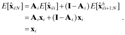
where Ai is the weighting matrix to be determined and ![]() is the state estimate from the backward filter at time ti using measurements from ti+1 to tN. Notice that weighting of
is the state estimate from the backward filter at time ti using measurements from ti+1 to tN. Notice that weighting of ![]() is (I − Ai) so that the smoothed estimate is unbiased if the individual filter estimates are unbiased:
is (I − Ai) so that the smoothed estimate is unbiased if the individual filter estimates are unbiased:
The minimum variance smoother solution is obtained by minimizing the trace of the error covariance for ![]() ; that is,
; that is,
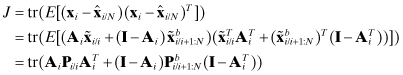
where ![]() and
and ![]() . The minimum is obtained by setting
. The minimum is obtained by setting
![]()
or
(9.2-19)
![]()
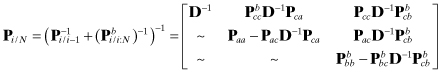
Thus
are the smoothed estimate and covariance at time ti given the estimates from the forward and backward filters. Notice that covariance Pi/N will be smaller than either Pi/i or ![]() , which shows the benefit of smoothing. Also notice that it is necessary to store all state estimates and covariance matrices from the forward filter (or alternatively from the backward filter) in order to compute the smoothed estimates.
, which shows the benefit of smoothing. Also notice that it is necessary to store all state estimates and covariance matrices from the forward filter (or alternatively from the backward filter) in order to compute the smoothed estimates.
The forward-backward filter solution to the smoothing problem is often used to derive other smoothing properties, but it is seldom implemented. Notice that the backward filter cannot use prior information because that would introduce correlation between forward and backward filter errors. The requirement for a prior-free filter operating backward in time implies that it should be implemented as an information filter using ![]() , rather than the covariance
, rather than the covariance ![]() . Then equation (9.2-20) is modified to avoid inversion of
. Then equation (9.2-20) is modified to avoid inversion of ![]() . See Fraser and Potter (1969) for the details, but note that the listed equation for the backward filter time update of the information matrix should be
. See Fraser and Potter (1969) for the details, but note that the listed equation for the backward filter time update of the information matrix should be

Other sources for information on the forward-backward smoother derivation include Maybeck (1982a, section 8.4) and Simon (2006, section 9.4.1).
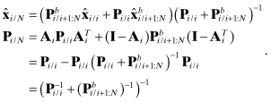
Example 9.3: Two-State Forward-Backward Smoothing
Figure 9.5 shows the 1 − σ “position” (state #1) uncertainty computed from the a posteriori filter and smoother covariance matrices for the two-state problem of Example 8.2 when using Q = 1. Notice that the uncertainty of both the forward and backward filters is initially large, but decays to a nearly constant value after processing about 10 s of data. As expected, the uncertainty of the smoother matches the forward filter uncertainty at the end time, and the backward filter at the initial time. The uncertainty of the smoother in the middle of the data span is much less than that of either the forward or backward filters.
FIGURE 9.5: Two-state forward filter, backward filter, and smoother 1-sigma position uncertainty.
Creation of a separate backward information filter with all the associated model structure makes the forward-backward smoother approach somewhat unattractive. Two more popular fixed-interval covariance-based smoothers are:
1. Rauch-Tung-Striebel (RTS) smoother: The state estimates, a priori covariance and a posteriori covariances (or equivalent information) from the forward filter are saved and used in a backward state/covariance recursion that is initialized with the final filter solution.
2. Modified Bryson-Frazier (mBF) smoother: The algorithm derived from the work of Rauch et al. is a more efficient form of a result reported by Bryson and Frazier (1963). Bierman (1977b) refers to it as mBF. Rather than using filter covariances to compute smoother gains, this approach uses a backward recursion of adjoint variables that avoids matrix inversions. Although the mBF smoother can be derived from the RTS algorithm, the information saved from the forward filter involves measurements rather than process noise.
These two smoothers are described in following sections. Chapter 10 discusses three “square-root” smoothers: the square-root information smoother (SRIS), the Dyer and McReynolds (1969) covariance smoother, and a square-root version of the RTS. A number of other smoothing algorithms are available but infrequently used. Surveys of smoothing algorithms are found in Meditch (1969, 1973), Kailath and Frost (1968), Kailath (1975), and Bierman (1974, 1977b).
In should be noted that the Kalman filter used to generate inputs for fixed-interval smoothers must be optimal. That is, a Kalman-Schmidt consider filter cannot be used because the state estimates are suboptimal, thus introducing correlations between forward and backward solutions that are not accounted for. There is a critical loss of information in using a consider filter that cannot be reconstructed in a backward sweep smoother.
9.2.3.1 RTS Smoother
Rauch et al. (1965) elegantly derived a backwardly recursive smoother using conditional probabilities and maximization of the likelihood function for assumed Gaussian densities. They showed that the joint probability density for the states at ti and ti+1 and measurements from t0 to the final time tN can be expressed using conditional probability densities as
![]()
where subscripts on p have been omitted to simplify the notation. By maximizing the logarithm of the above density using the time update model equations (8.1-4) and (8.1-5) to compute conditional densities, they found that ![]() is the solution that minimizes
is the solution that minimizes
![]()
That solution is obtained by setting the gradient to zero and using the matrix inversion identity of Appendix A. The RTS algorithm can also be derived from the forward-backward smoothing equations, as demonstrated by Simon (2006, section 9.4.2), or from the SRIS of Chapter 10.
The RTS backward recursion is
where the gain matrix is
and ![]() are generated from the Kalman filter and associated computations. The backward recursions are initialized with
are generated from the Kalman filter and associated computations. The backward recursions are initialized with ![]() and PN/N from the forward filter and repeated for i = N − 1, N − 2,…, 1. Although the gain matrix is usually written as equation (9.2-22), by rearranging the equation for the filter covariance time update equation (8.1-5) as
and PN/N from the forward filter and repeated for i = N − 1, N − 2,…, 1. Although the gain matrix is usually written as equation (9.2-22), by rearranging the equation for the filter covariance time update equation (8.1-5) as
![]()
the gain can be written as
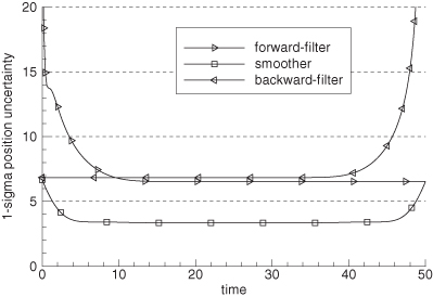
This equation directly shows that in the absence of process noise Q, smoothing is just backward integration. Furthermore, bias states that are not driven by process noise are not changed from the final filter estimate; that is, they are not smoothable. If the bias states are located at the bottom of the state vector, the gain matrix is
(9.2-24)
where we have used the same partitioning of dynamic and bias states shown in Section 9.2.1. The notation ![]() and
and ![]() refers to the dynamic-dynamic and dynamic-bias partitions of
refers to the dynamic-dynamic and dynamic-bias partitions of ![]() . When the fraction of bias states is significant and Qdd is sparse, this form of the gain matrix can greatly reduce computations, even though it does require inversion of Φdd.
. When the fraction of bias states is significant and Qdd is sparse, this form of the gain matrix can greatly reduce computations, even though it does require inversion of Φdd.
Since the required arrays can be computed in different forms, there are several options for saving output from the forward Kalman filter: the best choice for a particular problem depends on the number of dynamic and bias states and the sparseness of Φdd, Φdb and Qdd. It is generally efficient to write
![]()
from the forward filter to direct access disk after performing the filter time update at ti+1, but before performing the measurement update. When arrays are small and disk storage size is unimportant, Pi+1/i can also be saved. Otherwise it can be computed as ![]() . If equation (9.2-23) is used to compute the gain, Pi+1/i rather than Pi/i can be saved. Notice that
. If equation (9.2-23) is used to compute the gain, Pi+1/i rather than Pi/i can be saved. Notice that ![]() , so it may be more efficient when models are analytic to compute Φi,i+1 for a negative time step rather than to invert a matrix. To conserve storage, only the upper triangular portion of Pi/i or Pi+1/i should be written to the file. If the number of bias states is significant, only the nonzero partitions of Φi+1,i and Qi+1,i should be saved.
, so it may be more efficient when models are analytic to compute Φi,i+1 for a negative time step rather than to invert a matrix. To conserve storage, only the upper triangular portion of Pi/i or Pi+1/i should be written to the file. If the number of bias states is significant, only the nonzero partitions of Φi+1,i and Qi+1,i should be saved.
The RTS smoother is probably the most popular type of smoother. It is relatively easy to understand and implement, and the algorithm can be used to derive other types of smoothers. It does not require storage of measurement information, which makes it flexible: measurements may be processed in the filter one-component-at-a-time, or measurements types and sizes may be variable without any impact to the smoother. It can also be very efficient when the number of dynamic states is comparable to or smaller than the number of bias states.
One possible disadvantage of the RTS is numerical accuracy. The state and covariance differencing of equation (9.2-21) can result in a loss of precision when the quantities differenced are comparable in magnitude. However, there are two reasons why loss of numerical accuracy is rarely a problem. First, since fixed-interval smoothing is a post-processing activity, it is usually executed on computers having double precision floating point registers—such as the PC. Second, errors in computing the smoothed covariance Pi/N have no impact on the accuracy of the smoothed state ![]() since the gain matrix only uses quantities from the Kalman filter. In fact, Pi/N is sometimes not computed to reduce computational run time. Because of covariance differencing, there is the potential for the computed Pi/N to have negative variances, but this is rarely a problem when using double precision.
since the gain matrix only uses quantities from the Kalman filter. In fact, Pi/N is sometimes not computed to reduce computational run time. Because of covariance differencing, there is the potential for the computed Pi/N to have negative variances, but this is rarely a problem when using double precision.
Another problem is caused by the need to invert Pi+1/i or Φ or both. The iterations can lose accuracy if Φ has a negligibly small value on the diagonal—possibly because of data gaps causing propagation over a long time interval. To prevent the problem for long time integrations, either limit the maximum time step or set a lower limit on diagonal elements of Φ for Markov process states (when e−FT/τ is negligibly small).
9.2.3.2 mBF Smoother
This algorithm uses the adjoint variable approach from optimal control theory. The adjoint n-vector λ used in the mBF is equivalent to
(9.2-25)
![]()
(Rauch et al. showed that the mBF smoother can be derived from the RTS smoother using the above substitution: notice that the first line of equation (9.2-21) can be written as ![]() ) The mBF also computes an n × n adjoint matrix Λ that is used to calculate the smoothed covariance.
) The mBF also computes an n × n adjoint matrix Λ that is used to calculate the smoothed covariance.
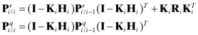
Starting at the final time tN with λN/N = 0 and ΛN/N = 0, a measurement update is performed to remove the effect of the last measurement from the adjoint variables for i = N:

where Hi, ![]() ,
, ![]() , Ki, and Φi,i−1 are generated from the Kalman filter. Then the backward time update
, Ki, and Φi,i−1 are generated from the Kalman filter. Then the backward time update
(9.2-27)
is evaluated, and smoothed estimates and covariances at ti−1 are computed as
Note: The ![]() variable used by Bierman is equal to the negative of our λi/i, and the wi variable of Rauch et al. is equal to our λi+1/i. The formulations presented by Bierman (1977b) and Rauch et al. (1965) both have minor errors, such as missing transpose operators or incorrect symbols. These or similar errors also appear in other papers. Equations (9.2-26) to (9.2-28) above have been numerically verified to match the RTS and forward-backward smoothers.
variable used by Bierman is equal to the negative of our λi/i, and the wi variable of Rauch et al. is equal to our λi+1/i. The formulations presented by Bierman (1977b) and Rauch et al. (1965) both have minor errors, such as missing transpose operators or incorrect symbols. These or similar errors also appear in other papers. Equations (9.2-26) to (9.2-28) above have been numerically verified to match the RTS and forward-backward smoothers.
As with the RTS smoother, these equations are repeated for i = N, N − 1,…, 2. Because measurements are explicitly processed in equation (9.2-26), this time index is shifted by +1 compared with the index used in the previous section, but the number of steps is the same. Notice that the mBF formulation uses the filter variables
![]()
but does not use Qi+1,i (as required in the RTS algorithm). The filter implementation should save these variables to direct access disk after computing Hi, Ci, Ki, and ![]() , but before measurement updating to compute
, but before measurement updating to compute ![]() and Pi/i. Notice that the mBF smoother does not use matrix inversions, but does require more n × n matrix multiplications than the RTS algorithm. As with the RTS algorithm, numerical errors in calculating the covariance Pi/N do not have any impact on the smoothed state estimate
and Pi/i. Notice that the mBF smoother does not use matrix inversions, but does require more n × n matrix multiplications than the RTS algorithm. As with the RTS algorithm, numerical errors in calculating the covariance Pi/N do not have any impact on the smoothed state estimate ![]() . Numerical accuracy may or may not be better than for the RTS algorithm. It is somewhat more difficult to take advantage of dynamic model structure in the mBF than in the RTS. Handling of measurements processed one-component-at-at-time in the Kalman filter is also more difficult with the mBF. This may explain why the RTS is more frequently used.
. Numerical accuracy may or may not be better than for the RTS algorithm. It is somewhat more difficult to take advantage of dynamic model structure in the mBF than in the RTS. Handling of measurements processed one-component-at-at-time in the Kalman filter is also more difficult with the mBF. This may explain why the RTS is more frequently used.
Example 9.4: Maneuvering Tank Tracking
This example uses the maneuvering tank data and six-state model of Section 3.2.1. Since both the measurement and dynamic models are nonlinear, the example demonstrates use of both the EKF and RTS smoothing. It was also used to test the iterated-filter-smoother, but results were essentially the same as those of the EKF.
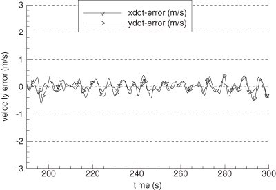
The reconstructed position data for the Scout vehicle is shown in Figure 9.6. A sensor measuring azimuth and range to the target tank was located at x = 600 m, y = –600 m. Also shown in the figure are lines from the sensor to the target at 190 and 300 s of tracking. (Although the filter and smoother processed the entire tracking span, performance is only shown for this shorter span so that plots are less cluttered.) The simulated 1 − σ noise was 0.3 milliradians for azimuth and 2 m for range. Process noise was only modeled on the alongtrack and crosstrack acceleration states, where the assumed power spectral density (PSD) was 1.0 and 0.5 m2/s5, respectively.
FIGURE 9.6: Tank ground track and sensor location.
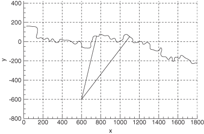
Figure 9.7 shows the error in EKF-estimated velocity states for the time span 190 to 300 s. Figure 9.8 is the comparable plot for the smoother velocity error. Notice that the smoother error is indeed “smoother” and also much smaller. The improvement of the smoother is much greater than would be expected from the approximate doubling of the number of measurements used for each state estimate. The relative filter/smoother reduction in peak position errors is approximately the same (4:1) as for velocity. Smoother alongtrack acceleration errors are about 40% smaller than those of the filter, but crosstrack acceleration error magnitudes are similar to those of the filter.
FIGURE 9.7: Error in filter-estimated tank velocity.
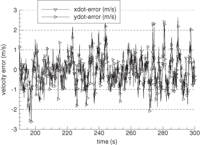
FIGURE 9.8: Error in smoother-estimated tank velocity.
Example 9.5: Tracking of Aircraft in Landing Pattern
A second example was described in Section 3.2.2. Motion of a small aircraft in the airport landing pattern was simulated using an eight-state model. A radar measuring range, azimuth, and elevation every second was located on the airport, where the simulated measurement noise 1 − σ was 1 m for ranges and 0.2 milliradian for angles. Vertical velocity, crosstrack acceleration, and alongtrack acceleration were modeled in the filter as random walk processes with input white process noise PSDs of 0.08 m2/s3, 1.0 m2/s5, and 0.4 m2/s5, respectively. This model for random perturbations is time-invariant, but actual perturbations on these parameters only occur for short intervals. These PSD values were selected to give “good” average performance.
Figures 9.9 and 9.10 show the error in EKF-estimated position and velocity versus time. Notice that distinct error patterns occur during the turns (at 45–55 and 76–87 s), changes in vertical velocity (at 76 and 90 s) and during deceleration (90–95 s). Figures 9.11 and 9.12 are the comparable plots for the smoother. The errors are much smaller, but significant error patterns remain during maneuvers. This demonstrates the difficulty in using a time-invariant process noise model to characterize state perturbations that are really step jumps. Use of a first-order Markov process rather than a random walk process model for the last three states did not improve performance significantly.
FIGURE 9.9: Error in filter-estimated aircraft position.
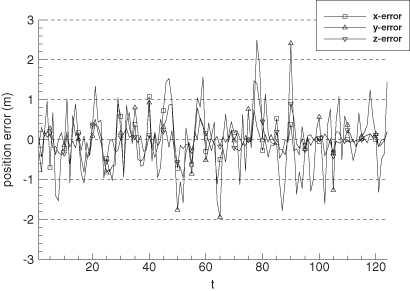
FIGURE 9.10: Error in filter-estimated aircraft velocity.
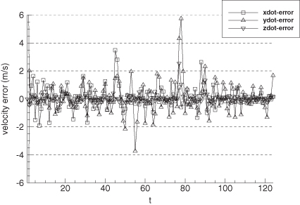
FIGURE 9.11: Error in smoother-estimated aircraft position.
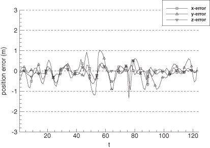
FIGURE 9.12: Error in smoother-estimated aircraft velocity.
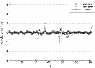
We also tested the iterated filter-smoother for this example, and results were essentially the same as for the EKF.
9.2.3.3 Pass Disposable Bias States in the RTS Smoother
In some applications individual sensors only acquire measurements for limited time spans, so measurement biases associated with these sensors need only be included in the filter state vector when the sensor is receiving data. Orbit determination is one such example because ground-based sensors only view low-altitude satellites for short periods of time, and may not see a satellite again for a day or more. Since a large component of the measurement bias is due to local tropospheric and ionospheric atmospheric effects or other time-varying errors, the biases can be treated as independent for different passes. The RTS algorithm has the ability to reconstruct pass-disposable bias states without the need to carry them continuously in the Kalman filter. Other smoothers—particularly information-based smoothers—probably have a comparable ability, but we have not seen algorithms for reconstructing the pass-parameters. Implementation of pass-disposable biases greatly reduces the filter/smoother computational and storage burdens since a few filter bias states can optimally handle hundreds of pass-disposable biases.
Tanenbaum (1977) discovered that information for bias states dropped by the filter can be reconstructed in the backward recursion of the RTS algorithm because the bias states are not smoothable. Tanenbaum derived the algorithm using the forward-backward smoother algorithm of Fraser and Potter, and then applied it to the RTS. The derivation has not been published, but because of space limitations we only summarize the results.
We first consider the state estimates obtained from forward and backward filters at a time point located between two station passes, as shown in Figure 9.13. The a priori information for the pass B biases is treated as a measurement that does not enter the forward filter until the pass begins. Hence the forward filter a priori estimate and covariance at ti have the form
where subscript c denotes states that are common to both the forward and backward filters and subscripts a and b refer to pass biases for the two passes. Since information on the pass B states is not available, the covariance is represented as infinity. The backward filter a posteriori estimate and covariance at ti are of the form

where a prior information is never used in the backward filter. Since the smoothed covariance is the inverse of the sum of information matrices for the two independent estimates, it has the form
where ![]() , and the symmetric lower triangular partitions are not shown. (Inversion of matrices containing infinity must be done with great care, but the result can be derived more rigorously starting with information arrays.) Notice that the solution for common parameters does not depend on pass-parameters, and the solution for pass A parameters does not depend on pass B (and vice versa). This verifies that it is not necessary to carry pass-parameters outside the pass, but does not yet show that they can be reconstructed in the backward sweep of the RTS smoother.
, and the symmetric lower triangular partitions are not shown. (Inversion of matrices containing infinity must be done with great care, but the result can be derived more rigorously starting with information arrays.) Notice that the solution for common parameters does not depend on pass-parameters, and the solution for pass A parameters does not depend on pass B (and vice versa). This verifies that it is not necessary to carry pass-parameters outside the pass, but does not yet show that they can be reconstructed in the backward sweep of the RTS smoother.
FIGURE 9.13: Estimation of smoothed pass-parameters.
We now consider what happens at point ti−1 which we assume is the time of the last measurement in pass A. The RTS algorithm uses the covariance difference at ti, which after some manipulation can be shown to have the form

where ![]() , but the actual common state covariance difference ΔPcc = (Pcc)i/N − (Pcc)i/i−1 is used in implementing the algorithm. (Covariances Pac and Pcc in equation [9.2-29] are obtained from the filter Pi/i−1, and
, but the actual common state covariance difference ΔPcc = (Pcc)i/N − (Pcc)i/i−1 is used in implementing the algorithm. (Covariances Pac and Pcc in equation [9.2-29] are obtained from the filter Pi/i−1, and ![]() are obtained from
are obtained from ![]() from the backward filter.) Values in the last row and column of equation (9.2-29) are irrelevant because they will not be used again in the backward sweep of the RTS. To avoid a growing smoother state size, these states should be eliminated from the smoother when they no longer appear in the filter state vector.
from the backward filter.) Values in the last row and column of equation (9.2-29) are irrelevant because they will not be used again in the backward sweep of the RTS. To avoid a growing smoother state size, these states should be eliminated from the smoother when they no longer appear in the filter state vector.
The above equation verifies that “missing” terms of Pi/N − Pi/i−1 can be reconstructed by pre- or post-multiplying ΔPcc by the factor ![]() obtained from the forward filter Pi/i−1. Hence pass-parameters should be discarded in the filter after writing
obtained from the forward filter Pi/i−1. Hence pass-parameters should be discarded in the filter after writing ![]() at ti to the disk. By a similar procedure it is shown that the difference in state estimates can be reconstructed as
at ti to the disk. By a similar procedure it is shown that the difference in state estimates can be reconstructed as
(9.2-30)
![]()
where the pass B states have been eliminated.
The last step in the reconstruction fills in the pass A terms of the RTS gain matrix. Again after some manipulation using equation (9.2-23), it can be shown that
(9.2-31)
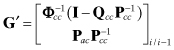
is the gain matrix to be used in
(9.2-32)
![]()
to reconstruct the missing pass A bias states from the a priori forward filter common states and covariance at time ti. The pass-disposable bias states to be added in the backward smoother sweep will not in general be located at the bottom of the filter state vector, and the smoother state vector will be smaller than the filter state when pass-parameters are added. Hence it is necessary to shift state and covariance ordering when implementing the reconstruction. This is greatly simplified if state labels are saved with the filter variables written to disk so that the location of common filter-smoother states can be identified. Software that implements this method is described in Chapter 13.
This algorithm was used operationally in orbit determination filter-smoothers at the U.S. Naval Surface Weapons Center and at the National Aeronautics and Space Administration (Gibbs 1979, 1982) to estimate pass-disposable bias states for hundreds of tracking passes using storage and computations for only a few biases.
Example 9.6: Global Positioning System (GPS) Satellite Navigation
The previous examples are of relatively low order, but it is also practical to use smoothers for large complex problems. Navigation for the GPS constellation of satellites is one such example. GPS and the navigation filter were described in Section 3.4.10.
A Kalman filter similar to the Master Control Station (MCS) navigation filter was used to process pseudo-range data from 19 ground receivers obtained during days 238 to 243 of 2005. An RTS smoother was also implemented and used for a 5 day span. To minimize disk storage and computations, it was desirable to explicitly take advantage of the sparseness in the state transition and process noise matrices, and to use pass-disposable monitor station biases, as described above. For the newest space vehicles in service at that time—designated as Block IIR—the smoothed satellite ephemeris typically agreed within 5–14 cm of the ephemeris computed by the International GNSS Service (IGS) using a much larger set of ground stations. We used the smoothed ephemeris as a reference to calculate the user range error (URE) of the filter-calculated ephemeris. The URE is defined for GPS as
![]()
where Δr, Δi, Δc are the radial, intrack, and crosstrack components of the ephemeris error, and Δt is the error in the calculated clock time multiplied by the speed of light. Figure 9.14 shows the zero-age-of-data (no prediction) URE calculated using the difference between filter and smoother ephemeris/clock states for Block IIR space vehicles. Notice that peak URE values are 23 cm, but average UREs are usually less than 10 cm. Certain space vehicles tend to have slightly greater UREs than others because of differences in clock stability.
FIGURE 9.14: Computed GPS user range error for 18 block IIR space vehicles.
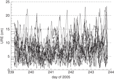
Since this example uses actual rather than simulated GPS measurements, the true errors in filter and smoother state estimates are unknown. Based on computed filter and smoother covariances, and on the smoother comparison with IGS results listed above, it is believed that most of the URE shown in Figure 9.14 is filter error.
9.3 FILTER ERROR ANALYSIS AND REDUCED-ORDER MODELING
Just as with least-squares processing, the formal error covariance Pi/i of the Kalman filter is a lower bound on estimate errors ![]() when process noise, measurement noise, and initial condition errors are correctly modeled in the filter. Actual errors may be larger when the filter model does not match reality, some states are deliberately not estimated, the gain matrix is suboptimal, or the effects of nonlinearities are not included. A more realistic estimate of
when process noise, measurement noise, and initial condition errors are correctly modeled in the filter. Actual errors may be larger when the filter model does not match reality, some states are deliberately not estimated, the gain matrix is suboptimal, or the effects of nonlinearities are not included. A more realistic estimate of ![]() —or even a distribution function—is important for several reasons. First, it is very useful in the design stage when attempting to develop a filter that meets accuracy requirements under realistic operating conditions. Availability of a realistic error covariance—particularly when contributions of different error sources are separately available—allows comparison of different designs and selection of the “best”. Second, knowledge of the true error covariance is of interest for its own sake. For example, it is often necessary to list expected accuracy when providing specifications for customers or when “proving” that the system meets specifications. Example accuracy specifications include 3 − σ error limits, confidence bounds, or probability of “impact.” Finally in systems where the filter output is used to make decisions on possible control actions, the error covariance or distribution can be a required input. For example, the estimate error covariance is sometimes required for risk analysis associated with potential response actions.
—or even a distribution function—is important for several reasons. First, it is very useful in the design stage when attempting to develop a filter that meets accuracy requirements under realistic operating conditions. Availability of a realistic error covariance—particularly when contributions of different error sources are separately available—allows comparison of different designs and selection of the “best”. Second, knowledge of the true error covariance is of interest for its own sake. For example, it is often necessary to list expected accuracy when providing specifications for customers or when “proving” that the system meets specifications. Example accuracy specifications include 3 − σ error limits, confidence bounds, or probability of “impact.” Finally in systems where the filter output is used to make decisions on possible control actions, the error covariance or distribution can be a required input. For example, the estimate error covariance is sometimes required for risk analysis associated with potential response actions.
As with least squares, there are two basic methods by which the statistical characteristics of the estimation errors may be determined: linear covariance analysis and Monte Carlo simulation. In covariance analysis, the effects of various error sources are propagated through the filter equations assuming that the error effects are additive and linear. The approach can also be applied to nonlinear systems, but error models are linearizations about the state trajectory. Covariance error analysis has the advantages that the effects of error sources may be separately computed, and it is computationally fast. However, coding effort may be significant. Monte Carlo error analysis is more rigorous because (1) it includes the effects of nonlinearities; (2) it can handle more complicated cases where there are significant structural differences between the filter model and a detailed “truth” model; and (3) it is easily coded. However, it is computationally slow since many random samples are necessary to properly characterize the error distribution. It is even slower when it is necessary to run separate simulations for each error source to separately determine the effects. The remainder of this section discusses options for linear covariance analysis.
Covariance error analysis is used when filter models of system dynamics and measurements are different from those of detailed truth models. In most cases the differences arise because the filter uses a ROM. There are a variety of reasons why filter models are of lower order than detailed simulation models. Since computations increase as the square or cube of filter order for most implementations, computational reduction is one of the primary reasons for using a ROM. Other reasons include improved computational accuracy (due to improved observability), imprecise knowledge of parameters used in detailed models, and improved robustness (in some cases).
Methods used to develop a ROM from a detailed model include the following:
1. Do not estimate (i.e., do not include in the filter state vector) various fixed parameters that are reasonably well known.
2. Eliminate detailed models of low-amplitude effects and instead increase Q or R if the errors are nearly random.
3. Same as above, but also modify coefficients in Φ to allow the filter to have a broader frequency response than the detailed model.
4. Average or subsample measurements so that the filter model need not include states that model high-frequency effects.
5. Replace complex random force models with colored noise (low-order Markov process) models.
6. Combine states having similar measurement signatures since observability of the separate parameters will be poor.
7. Replace distributed parameter models with lumped parameter models.
When a ROM simply deletes states of a detailed model, linear perturbation methods may be used to either analyze the effects of errors in unadjusted parameters on filter accuracy, or to “consider” the uncertainty of the parameter values when weighting the measurements. However, when a filter model uses states and parameters different from those of a detailed model, the above approach is not directly applicable. Alternate forms of covariance error analysis can be used when the filter model states are a linear transformation of detailed model states, or when the filter model and detailed model have a subset of states in common. When the filter model has a different structure than a detailed model, Monte Carlo simulation is often the only option for error analysis.
We present three approaches for linear covariance error analysis of the Kalman filter. The first is used when the filter model structure closely matches reality, but some parameters of the model may be unadjusted or treated as consider parameters. Linearized sensitivity and covariance matrices for the effects of five possible error sources are summed to compute the total error covariance. The approach also computes derivatives of the measurement residuals with respect to unadjusted parameters. The second approach is used when the filter ROM is a linear transformation on a more accurate representation of the system. It is assumed that the transformation is used to generate reduced-order filter versions of the Φ, Q, and H matrices. Then the adjusted states and unadjusted parameters of the transformed model are analyzed using the first approach. The third approach is used when the filter values and possibly structure of the Φ, Q, H, and R arrays are different from those of the detailed model, but a subset of important states are common to both models. In this case error propagation can be analyzed using an augmented state vector that includes both the detailed and reduced-order state vectors.
Extended discussions of ROM philosophy appear in Maybeck (1979, chapter 6), Grewal and Andrews (2001, section 7.5), Gelb (1974, chapter 7), and to a lesser extent in Anderson and Moore (1979, chapter 11) and Simon (2006, section 10.3). We encourage you to read one or more of these books. To summarize, ROM is a trade-off between developing a model that
1. accurately characterizes the system and provides excellent estimation performance when all parameters of the model are correct, but may deteriorate rapidly when model parameters are incorrect, versus
2. a model that provides somewhat lower accuracy under the best conditions but deteriorates less rapidly when model parameters are wrong.
The trade-off between computations and performance may also be a factor. A ROM may be less sensitive to parameter errors than a higher order model, but that is not necessarily true. Covariance error analysis can be invaluable in evaluating the trade-offs, but ultimately Monte Carlo analysis should be used to verify the performance.
9.3.1 Linear Analysis of Independent Error Sources
This section derives linear error effects in the discrete-time Kalman filter due to un-estimated bias parameters, Schmidt-type consider bias parameters, measurement noise, process noise, and the initial estimate. The following derivation is mostly due to Aldrich (1971) and Hatch (Gibbs and Hatch 1973), partly based on work by Jazwinski (1970, p. 246) and Schmidt (1966). This presentation assumes that the unadjusted and consider parameters are biases, so errors can be modeled using linear sensitivity arrays. The same approach can also handle unadjusted and consider states that are colored noise (rather than biases), but it is necessary to instead carry error covariance components rather than sensitivity arrays.
The error in the a posteriori state estimate at time ti−1 is assumed to be a linear function of five statistically independent error sources:
(9.3-1)
![]()
where
| is the state error due to errors in filter values ( | |
| is the state error due to errors in filter values ( | |
| is the state error due to errors in the initial filter estimate | |
| is the state error due to cumulative errors in measurement noise, and | |
| is the state error due to cumulative errors in process noise. |
(Superscripts are used in this section to denote components of a total vector or array.) There are no restrictions on the effects of unadjusted-analyze and consider parameters: they may appear in the force model, the measurement model, or both.
It is further assumed that the error in ![]() due to static parameters can be represented using linear sensitivity arrays:
due to static parameters can be represented using linear sensitivity arrays:
(9.3-2)
where ![]() ,
, ![]() , and
, and ![]() . All error sources are assumed to be zero mean and independent.
. All error sources are assumed to be zero mean and independent.
Time propagation of the true state at time ti is modeled as
(9.3-3)
![]()
The time subscripts have been dropped from partitions of Φ to simplify notation. The corresponding filter time update is
(9.3-4)
![]()
so errors propagate as
(9.3-5)
where
(9.3-6)
Defining the portions of the total error covariance due to measurement and process noises as
and noting that the error sources are assumed to be independent, the true error covariance is
where ![]() ,
, ![]() ,
, ![]() , and
, and ![]() . Again we drop the time subscript from Q and subsequent H and R arrays for simplicity in notation, not because they are assumed constant. From equation (9.3-7) the portions of Pi/i−1 due to measurement and process noise are, respectively,
. Again we drop the time subscript from Q and subsequent H and R arrays for simplicity in notation, not because they are assumed constant. From equation (9.3-7) the portions of Pi/i−1 due to measurement and process noise are, respectively,
The sensitivity and covariance arrays are initialized as follows:
(9.3-9)
![]()
The filter model of the state error covariance ![]() is the same as equation (9.3-7) without the
is the same as equation (9.3-7) without the ![]() term. (Superscript “f” denotes filter model.)
term. (Superscript “f” denotes filter model.)
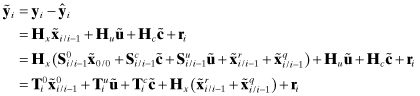
The true measurement model is
(9.3-10)
![]()
and the filter prediction is
(9.3-11)
![]()
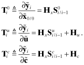
so the measurement residual is
(9.3-12)
where the measurement residual derivatives for the static errors are
(9.3-13)
These residual derivatives can be very helpful when trying to determine types of model errors that can cause particular signatures in measurement residuals. However, the T arrays should be multiplied by the expected standard deviation for each parameter (e.g., ![]() for diagonal Pu) before plotting as a function of time. In other words, compare the observed residual signatures with expected perturbations (not derivatives) due to each unadjusted parameter.
for diagonal Pu) before plotting as a function of time. In other words, compare the observed residual signatures with expected perturbations (not derivatives) due to each unadjusted parameter.
The true residual error covariance is
(9.3-14)
![]()
However, the filter does not know about unadjusted error parameters, and thus models the residual covariance as
(9.3-15)
![]()
The Kalman gain matrix for adjusted states (with consider parameter) is computed as
(9.3-16)
![]()
where
(9.3-17)
![]()
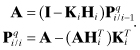
is the filter-modeled covariance of ![]() . (Note: significant computational saving may be obtained by grouping and saving matrix products for use in multiple equations.) The a posteriori state estimate is
. (Note: significant computational saving may be obtained by grouping and saving matrix products for use in multiple equations.) The a posteriori state estimate is
(9.3-18)
![]()
and the error is
(9.3-19)

where the a posteriori sensitivity arrays are
(9.3-20)
The recursions for those portions of the covariance matrix due to measurement and process noise are
and the total error covariance ![]() (including effects of unadjusted-analyze parameter errors) is
(including effects of unadjusted-analyze parameter errors) is
(9.3-22)
![]()
The filter model of the a posteriori error covariance is the same without the ![]() term.
term.
Notice that when the number of measurements is smaller than the number of states, significant computational reduction is obtained by implementing equation (9.3-21) as
![]()
and
The effort required to code the above equations expressed in matrix partitions is considerable. (Chapter 13 describes flexible code developed for this purpose—module COVAR_ANAL—where all static parameters may be selected by input as either adjusted, consider, or unadjusted-analyze.) If it is not necessary to know the separate contributions of measurement noise, process noise, and initial estimate errors, these terms may be combined into a single covariance, as normally done in a Kalman filter. That is, delete the ![]() and
and ![]() terms, rename the
terms, rename the ![]() term as
term as ![]() (initialized with
(initialized with ![]() ), replace equation (9.3-8) with
), replace equation (9.3-8) with
![]()
and replace equation (9.3-21) with
![]()
Also, coding is simpler and potentially more efficient if states in the global model are ordered as dynamic-core, dynamic-bias, and measurement-bias. With this ordering, the state transition, process noise, and measurement model matrices have the forms
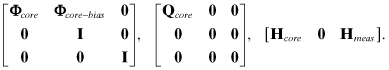
Then
Φxx is formed as Φcore plus selected columns of Φcore−bias, with added zero columns and 1’s placed on the diagonal,
Qxx is formed as Qcore plus zero row/columns,
Φxu and Φxc are formed by mapping columns of Φcore−bias and adding zero columns,
Hxx is formed as Hcore plus selected columns of Hmeas and zero columns,
Hu and Hc are formed by mapping columns of Hmeas and adding zero columns.
Example 9.7: Strapdown Inertial Navigation System
This example uses the 27-state model of a strapdown inertial navigation system discussed in Section 3.3. Recall that this model includes three states each for nine groups: errors in computed position, velocity, gyro tilt, accelerometer bias, accelerometer scale factor error, gyro bias, gyro scale factor error, gyro G-sensitive errors, and G-squared-sensitive errors. Simulated error magnitudes were listed in Section 3.3. The acceleration profile shown in Figure 3.3 was obtained for a simulated 790 s trajectory of a ballistic missile. There are multiple periods in which the acceleration changes because of booster staging or intentional bus maneuvers.
Position measurements generated by the simulation were processed by a Kalman filter that implemented the error equations of this section. The software allowed each of the 27 states to be individually selected as ignore, unadjusted-analyze, consider, or estimated. Initially only the first 15 states (position, velocity, tilt, accelerometer bias, and accelerometer scale factor) were estimated, with all remaining states set as unadjusted-analyze. Figure 9.15 shows the covariance-computed uncertainty in the x-component of position error due to each error source. Uncertainty signatures for the y and z components are similar. The lines are labeled as follows:
“sig0-delPx” is the 1 − σ uncertainty due to errors in the initial state estimate
“sigu-delPx” is the 1 − σ uncertainty due to errors in unadjusted-analyze parameters
“sigc-delPx” is the 1 − σ uncertainty due to errors in consider parameters
“sigr-delPx” is the 1 − σ uncertainty due to measurement noise
“sigq-delPx” is the 1 − σ uncertainty due to process noise
FIGURE 9.15: x-Position uncertainty versus time with 15 estimated states (12 unadjusted).

Since consider parameters were not included in this filter scenario, consider error effects are zero. Although difficult to see in the plot, the contribution of initial condition errors is negligible because the accuracy of the first measurement (0.61 mm 1 − σ) is much greater than the initial position error (4000 mm). The effects of process noise are also very small for the assumed process noise magnitudes. Uncertainty due to measurement noise (about 0.5 mm) is only slightly smaller than the measurement noise for a single measurement. However, the effect of errors in unadjusted-analyze parameters is quite large. Figure 9.16 is a similar plot for the x-component of velocity. The error behavior for velocity is similar to that of position, although the effects of process noise (0.06 mm/s after 200 s) are slightly larger than those of measurement noise (0.04 mm/s).
FIGURE 9.16: x-Velocity uncertainty versus time with 15 estimated states (12 unadjusted).
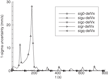
Filter errors were next analyzed with various sets of unadjusted parameters changed to consider. The effects of errors in individual unadjusted parameters can be determined by examining columns of the ![]() array multiplied by the corresponding uncertainty of
array multiplied by the corresponding uncertainty of ![]() for each parameter. Gyro biases had the largest effect, so they were made consider parameters. Figures 9.17 and 9.18 show the results: the error magnitudes are greatly reduced because inclusion of gyro bias consider parameters reduced the error sensitivity. In Figures 9.19 and 9.20 the gyro biases were estimated rather than considered. Notice that the errors increased greatly compared with Figures 9.17 and 9.18, and this result was confirmed by actual estimation errors of limited Monte Carlo trials. In other words, the position and velocity error magnitudes are actually larger when the gyro biases are estimated rather than considered. This counterintuitive result only occurs because other gyro errors (scale factor and acceleration-sensitive parameters) are unadjusted. When all 27 variables are adjusted (not plotted), the maximum errors after the boost phase are reduced to about 0.5 mm for position and 0.07 m/s for velocity. This demonstrates that the Kalman filter is “optimal” (meaning that errors are smallest) when all variables are estimated, provided that no other modeling errors exist. When modeling errors are present, errors in estimated states may not necessarily be smallest when all variables are estimated. In this example, treating the gyro bias parameters as consider parameters—rather than estimated—reduced the sensitivity of other estimated states to modeling errors caused by ignoring unadjusted parameters.
for each parameter. Gyro biases had the largest effect, so they were made consider parameters. Figures 9.17 and 9.18 show the results: the error magnitudes are greatly reduced because inclusion of gyro bias consider parameters reduced the error sensitivity. In Figures 9.19 and 9.20 the gyro biases were estimated rather than considered. Notice that the errors increased greatly compared with Figures 9.17 and 9.18, and this result was confirmed by actual estimation errors of limited Monte Carlo trials. In other words, the position and velocity error magnitudes are actually larger when the gyro biases are estimated rather than considered. This counterintuitive result only occurs because other gyro errors (scale factor and acceleration-sensitive parameters) are unadjusted. When all 27 variables are adjusted (not plotted), the maximum errors after the boost phase are reduced to about 0.5 mm for position and 0.07 m/s for velocity. This demonstrates that the Kalman filter is “optimal” (meaning that errors are smallest) when all variables are estimated, provided that no other modeling errors exist. When modeling errors are present, errors in estimated states may not necessarily be smallest when all variables are estimated. In this example, treating the gyro bias parameters as consider parameters—rather than estimated—reduced the sensitivity of other estimated states to modeling errors caused by ignoring unadjusted parameters.
FIGURE 9.17: x-Position uncertainty versus time with 15 estimated states and 3 consider parameters (9 unadjusted).
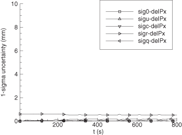
FIGURE 9.18: x-Velocity uncertainty versus time with 15 estimated states and 3 consider parameters (9 unadjusted).
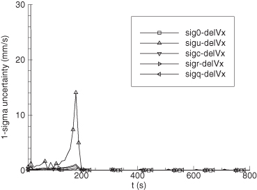
FIGURE 9.19: x-Position uncertainty versus time with 18 estimated states (9 unadjusted).
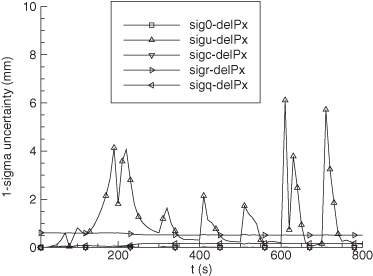
FIGURE 9.20: x-Velocity uncertainty versus time with 18 estimated states (9 unadjusted).
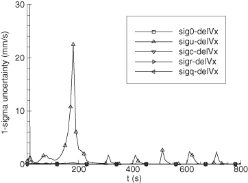
This example shows how the error analysis technique of this section can be applied to a realistic problem, and used to determine the best choice of estimated states and consider parameters for a ROM.
9.3.2 Error Analysis for ROM Defined as a Transformed Detailed Model
When the ROM simply deletes states of the detailed model, methods of the previous section may be used to either analyze the effects of errors in unadjusted parameters on filter accuracy, or to “consider” the uncertainty of the parameter values when weighting the measurements. However, when the filter model uses states and parameters different from those of the detailed model, the above approach is not directly applicable. The more general case will be discussed in the next section, or when that does not apply, Monte Carlo analysis can be used. When filter model states are a linear transformation of detailed model states, the covariance error analysis of the previous section can still be used provided that a preprocessing step is first applied, as will now be shown.
Let the detailed model states be denoted by xd of dimension nd and the filter states be denoted by xf of dimension nf < nd, where xf = Tfxd and Tf is nf × nd. An invertible transformation between the two state vectors must exist to analyze error propagation, so we instead assume that an augmented state vector xt of dimension nd is defined as
(9.3-23)
![]()
where (nd − nf) × nd matrix Ta is chosen to make
full rank. Also Ta must not transform states driven by process noise if it is used in the error analysis of the previous section. Otherwise the definitions of a and Ta are nearly arbitrary. There are a variety of approaches for chosing Tf. For example, it may sum xd states that have similar effects, or combine states to compute variables of interest (perhaps for control purposes), or may be composed of eigenvectors of the steady-state filter covariance for xd corresponding to the largest (poorly observable) eigenvalues.
Using the state transformation of equation (9.3-24), the state transition, state noise, measurement sensitivity matrices, and initial covariance for a model based on xt become
(9.3-25)

where Φd, Qd, and Hd are the model matrices for the detailed model. It is now conceptually simple to use xt as the total parameter set from which adjusted states (xf), unadjusted-analyze, and consider states are selected. These selections are then used in the error analysis equations of the previous section; that is, the appropriate partitions of the Φt, Qt, Ht, and (Pt)0/0 arrays for the corresponding states or parameters are substituted in the error equations. Since those error equations assume that unadjusted-analyze and consider parameters are biases (rather than dynamic states driven by process noise), a must include only biases, which explains why Ta must only transform biases. If the equations of the previous section are modified to include colored noise unadjusted-analyze and consider states, the restrictions may be relaxed.
9.3.3 Error Analysis for Different Truth and Filter Models
When the filter model has states and structure different from those of a detailed model, Monte Carlo simulation is often the only option for error analysis. However, if a subset of states are common to both filter and detailed models—even if the dynamic or measurement models have different structures and coefficients—it is possible to implement covariance error analysis using a dual-state model approach. (See Gelb 1974, or Grewal and Andrews 2001, for other examples.)
It is assumed that the detailed model is of the form
(9.3-26)
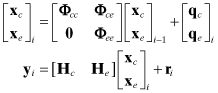
where xc represents a combination of dynamic and static states that are also used in the filter, and xe represents dynamic and static states that do not appear in the Kalman filter. For simplicity we assume that Φec = 0 (xc states do not drive the dynamics of xe), but that is not an inherent limitation of the method. It is also assumed that
(9.3-27)
![]()
E[qc] = 0, E[qe] = 0, E[ri] = 0, ![]() , and
, and ![]() . The Qce term may be zero in some problems.
. The Qce term may be zero in some problems.
The corresponding filter models are
(9.3-28)
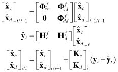
where Kc and Kd are the Kalman gain for the given system model defined by Φf, Qf, Hf, Rf, and P0/0. It is further assumed that ![]() has the same dimension and state definitions as xc, but no relationships between
has the same dimension and state definitions as xc, but no relationships between ![]() and Φcc, or
and Φcc, or ![]() and Hcc, are assumed. There are also no assumptions about relationships between
and Hcc, are assumed. There are also no assumptions about relationships between ![]() and xe: they may have different dimensions and state definitions. This allows for the possibility that
and xe: they may have different dimensions and state definitions. This allows for the possibility that ![]() is a colored noise and bias model of a larger model based on states in xe.
is a colored noise and bias model of a larger model based on states in xe.
The two separate models are concatenated and “common” states are differenced to give an augmented state vector represented as z. The dynamic model for z is
(9.3-29)
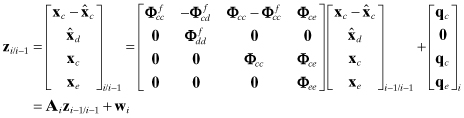
where
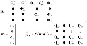
Notice that process noise does not drive the ![]() or
or ![]() states since the filter state time update does not include a random noise term. (It is of course modeled in the covariance time update used in computing the Kalman gain.) If we treat the initial states of the true model (xc_0 and xe_0) as fixed-but-unknown (nonrandom) parameters, the expected value of z0/0 is
states since the filter state time update does not include a random noise term. (It is of course modeled in the covariance time update used in computing the Kalman gain.) If we treat the initial states of the true model (xc_0 and xe_0) as fixed-but-unknown (nonrandom) parameters, the expected value of z0/0 is
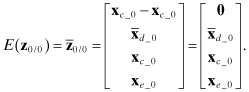
Since xd_0 is not required to represent physical variables, a “true” value of xd_0 does not really exist. However, we can assume that ![]() represents a reasonable guess for the mean value of those states. Then
represents a reasonable guess for the mean value of those states. Then ![]() can be computed by propagating
can be computed by propagating ![]() without the effects of process noise or measurement noise. Thus the covariance of zi/i−1 is
without the effects of process noise or measurement noise. Thus the covariance of zi/i−1 is
(9.3-31)
![]()
initialized with
(9.3-32)
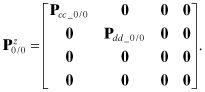
The arrays Pcc_0/0 and Pdd_0/0 should normally be equal to the state covariances used to initialize the filter. Again notice that Pdd_0/0 does not really exist since ![]() is not a physical state, but Pdd_0/0 must be specified to initialize the Kalman filter, so one hopes that it reasonably characterizes the effective errors in the filter model.
is not a physical state, but Pdd_0/0 must be specified to initialize the Kalman filter, so one hopes that it reasonably characterizes the effective errors in the filter model.
The detailed measurement model is represented using state vector zi/i−1 as
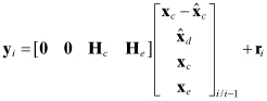
and the filter measurement model is
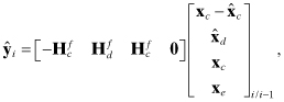
so the measurement residual used in the Kalman filter can be written as
(9.3-33)
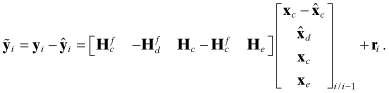
Now using ![]() in the Kalman filter update equation (8.1-11) yields the a posteriori state zi/i:
in the Kalman filter update equation (8.1-11) yields the a posteriori state zi/i:
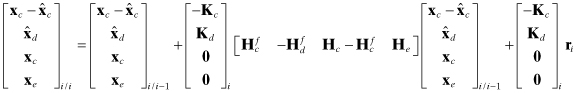
or
(9.3-34)
![]()
where
(9.3-35)
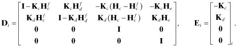
Thus the error covariance for zi/i is
Equations (9.3-30) and (9.3-36) give the time and measurement updates of the z covariance. The upper left nf × nf partition gives the error covariance ![]() for the common states, which is the desired output. Since “true” values of
for the common states, which is the desired output. Since “true” values of ![]() do not exist, it not possible to compute an error covariance for these filter states.
do not exist, it not possible to compute an error covariance for these filter states.
9.4 MEASUREMENT PREPROCESSING
As noted in Chapter 8, hypothesis tests on filter innovations can be quite effective in identifying and removing outlying measurements. However, these residual tests are relatively insensitive during the initialization period when the filter gain is high. Another reason for concern is the IIR characteristic of the Kalman filter. Unedited anomalous measurements can cause significant errors in the filter estimates for an extended period of time. For these reasons it is important that an operational system edit measurements before processing with a Kalman filter.
The methods available for measurement preprocessing and editing are mostly the same as described in Section 7.5 for least squares. High-rate data can be averaged or smoothed, and measurement editing logic can be included as part of the averaging/smoothing operation. Alternately, batch least squares can be used to compute parameter estimates (e.g., polynomial coefficients) and covariances that model an assumed deterministic evolution of the measurements over a short time span. The parameter estimates and covariance are used as measurements in the Kalman filter. This is called a mini-batch approach.
A low-order filter operating on raw measurement data can detect jumps and either edit individual measurements or alert the Kalman filter that parameter values may have jumped (thus allowing the filter to switch to a high-Q model or otherwise compensate for the jump.) Known measurements errors can be removed or known transformations applied in the preprocessing. When multiple measurements provide some redundancy, measurements may be compared to determine if all are consistent. This method is used in GPS ground system preprocessing to detect unexpected satellite and ground clock timing errors.
9.5 SUMMARY
Most Kalman filtering applications are for nonlinear systems. The EKF handles the nonlinearities by linearizing about the current estimate at each measurement update. The EKF is by far the most commonly used nonlinear method, and it works well for most applications. However, the estimate may be biased because the nonlinearities can cause the conditional probability density to become nonsymmetric. The linearized Kalman filter linearizes the model about a reference trajectory that is not updated after each measurement. It is used in cases (such as orbit determination) when it is possible to compute an accurate reference trajectory over an extended period of time. The IEKF is an extension of the EKF that re-linearizes and iterates the measurement update step when the measurement model is nonlinear. The iterated linear filter-smoother works similarly, but iterates on both the time update and measurement update steps when both models are nonlinear. These iterated filters are designed to compute the conditional mode rather than the conditional mean. They have the potential to work better than the EKF but there are few examples demonstrating improved performance. Also the iterations may not converge or may converge slowly. Other nonlinear techniques include higher order derivatives of the models when attempting to compute the mean of the conditional probability. Unfortunately these methods are only feasible for simple models and they seldom work well. Statistically linearized methods use describing functions to model the effective linear behavior of the model. Two other nonlinear filtering methods (described in Chapter 11) evaluate the model states at multiple points to better characterize the conditional probability density function.
Smoothing solutions compute the MMSE state at specific times using measurements both before and after the time of the smoothed state. Fixed-point smoothers only compute the state estimate at a fixed time. Several implementations are possible: the simplest augments the smoothed state (or a subset of states) with a copy of the current state at the desired smoothing time. Fixed-lag smoothers compute the smoothed state at a fixed time interval behind the measurements, and can operate as real-time processors. They are implemented either by augmenting and shifting the state vector, or using a chain of matrix multiplications over the lag time. These fixed-lag smoothers can be computationally expensive for real-time applications. Fixed-interval smoothers operate as post-processors and are implemented using a backward recursion to process outputs generated by the forward filter. The forward-backward filter due to Fraser and Potter is useful for theoretical purposes but is rarely implemented. The RTS and mBF methods are the most popular covariance-based fixed-interval smoothers. The state estimates and covariances (or equivalent information) from the forward filter are saved and used in a backward state/covariance recursion that is initialized with the final filter solution. The mBF uses adjoint variables in the backward recursion to avoid matrix inversions, but it is somewhat less flexible than the RTS. Both methods usually work well with high (but not excessive) computational burdens. An implementation of the RTS method was shown in Example 9.6 to work with disposable pass-dependent biases. Other types of smoothers will be discussed in the next chapter.
There are several reasons for analyzing the effects of various error sources on filter accuracy. Error analysis is very useful when designing filters to meet accuracy requirements under realistic operating conditions. A breakdown of the effects of the different error sources can help identify parameters to be adjusted in a ROM. This analysis is also helpful when attempting to design filters that are relatively insensitive to assumptions about model and filter parameter values. In some cases realistic error analysis is a required output when “proving” to a customer that the system meets accuracy specifications, or when providing input that is used for subsequent actions, such as control.
As with least-squares estimation, Monte Carlo and linear covariance error analysis can be used. Covariance error analysis can separately compute the effects of error sources and is computationally fast. Monte Carlo error analysis is more rigorous because it includes the effects of nonlinearities, can handle more complicated cases where there are significant structural differences between the filter model and a detailed “truth” model, and it is easily coded. Options for linear covariance error analysis include perturbation analysis of independent error sources (measurement noise, process noise, and errors in unadjusted or “considered” model parameters), analysis of ROM models defined as transformations on more accurate models, and analysis of truth and filter models that are structurally different but have a common subset of important states. In the latter case error propagation can be analyzed using an augmented state vector that includes state vectors for both models.
Section 9.3 also discussed methods for developing a ROM, and design considerations that impact selection of states. The goal of ROM development is usually to develop a high-accuracy filter that is insensitive to model parameter assumptions, or has greatly reduced computational requirements with minimal accuracy loss. Covariance error analysis can be invaluable when analyzing the trade-offs, but ultimately Monte Carlo analysis should be used to verify the performance for nonlinear systems.