
CHAPTER 3
MODELING EXAMPLES
This chapter presents several examples showing how the concepts of the previous chapter are applied to real problems. The models are also used as the basis of estimation examples in the remaining chapters. The reader may wish to skim this chapter, but refer back to these models when later examples are discussed.
The included examples are
1. Passive angle-only tracking of linear-motion ship or aircraft targets
2. Maneuvering tank tracking using multiple models
3. Aircraft tracking with occasional maneuvers
4. Strapdown inertial navigation
5. Spacecraft orbital dynamics
6. A fossil-fueled power plant
3.1 ANGLE-ONLY TRACKING OF LINEAR TARGET MOTION
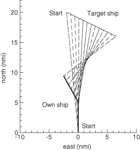
Figure 3.1 shows the basic scenario for passive tracking of a target ship moving in a straight line—sometimes called target motion analysis (TMA). This is typical of cases in which a ship is using passive sonar to track another ship or submarine. Since sonar is passive to avoid detection, the only measurements are a time series of angle measurements—range is not available. This example is also typical of cases where aircraft emissions are passively tracked from another aircraft. The angle measurements are used in a batch least-squares solution to compute four states: the initial east (e) and north (n) positions and velocities of the target: xt = [pte0 ptn0 vte vtn]T. Notice that the “own-ship” (tracking ship) must make at least one maneuver in order to compute a solution. The 30-degree left maneuver shown may not be operationally realistic since actual maneuvers are a compromise between obtaining a good solution and possibly being in a position to engage the target. While this case may seem trivially simple, it is of great interest for evaluating estimation methods because, without knowledge of range, the nonlinearities of the angle measurements are severe and nonlinear optimization can be difficult. The solution also breaks down when the target makes a maneuver, and that is difficult to detect without another source of information. Changes in received sonar signals may provide that information.
FIGURE 3.1: Passive tracking scenario.
The dynamic model for this problem is
(3.1-1)
and the measurement model at time ti is
(3.1-2)
where poe(ti) and pon(ti) are the own-vehicle east and north position at ti. Notice that because the dynamic model is so simple, the dynamics have been incorporated directly into the measurement model. The partial derivatives of the measurement with respect to the epoch target state are
(3.1-3)
![]()
where
| Δe | = pte0 + vteti − poe(ti), |
| Δn | = ptn0 + vtnti − pon(ti), and |
| R2 | = (Δe)2 + (Δn)2. |
For the example shown in Figure 3.1, the target ship is initially at a distance of about 20 nautical miles (nmi), and is moving at a constant velocity of 18.79 knots (kn) at a southeast heading of 115 degrees from north. The own-ship is initially moving directly north at a constant velocity of 20 kn. The own-ship measures bearing from itself to the target every 15 s, with an assumed 1 − σ accuracy of 1.5 degrees. At 15 min the own-ship turns 30 degrees to the left, and the encounter duration is 30 min. This example is used in Chapters 7 and 9 to demonstrate nonlinear estimation methods.
3.2 MANEUVERING VEHICLE TRACKING
This section discusses tracking models for two different types of maneuvering targets: tanks and aircraft. When in combat situations tanks tend to follow either high-speed straight line (constant velocity) paths, or moderate-speed serpentine paths to minimize the probability of being hit by enemy fire. Hence multiple types of motion are possible, but each motion type is fixed for periods of several seconds. The tank motion may be best tracked using multiple model filters where the best model for a fire control solution is selected using a tracking accuracy metric.
Civilian aircraft primarily fly constant velocity paths for extended periods of time, but occasionally turn, change speed, or climb/descend for periods of tens of seconds. When tracking aircraft for traffic control or collision avoidance purposes, a constant velocity model is optimal for possibly 90% of the tracking time, but occasionally constant rate turns, constant longitudinal acceleration, or constant rate of climb/descent will occur for short periods of time. Hence the tracking can be characterized as a “jump detection” problem, with associated state correction when a jump is detected.
3.2.1 Maneuvering Tank Tracking Using Multiple Models
Tank fire control algorithms are usually based on the assumption that the target vehicle moves in a straight line during the time-of-flight of the projectile. However, military vehicles are capable of turning with accelerations of 0.3 to 0.5 g and their braking capability approaches 0.9 g. At ranges of 1 to 3 km, projectile time-of-flights vary from 0.67 to 2 s. Thus target vehicle maneuvering can significantly reduce the hit probability when tracked by a constant velocity tracker. This explains the interest in higher-order adaptive trackers.
In 1975 the U.S. Army conducted an Anti-Tank Missile Test (ATMT) where accurate positions of moving vehicles were recorded using three vehicles: an M60A1 tank, a Scout armored reconnaissance vehicle, and a Twister prototype reconnaissance vehicle. The M60A1 is a heavy tank and the least maneuverable, while the Twister is the most maneuverable. The drivers were instructed to maneuver tactically at their own discretion. They were also required to make maximum use of terrain and to break the line-of-sight to the gun position. The maneuvers consisted of short dashes, random serpentine, and fast turns. Drivers rarely followed the same paths used in previous tests.
The results from those tests showed that typical vehicle motions were very dependent upon the capabilities of the vehicle. Drivers tended to use the full maneuvering capability of the vehicle. For example, the magnitude of the serpentine motion was greater for the Twister than for the M60A1, and the maneuver frequency was higher. This suggested that a multiple-model adaptive tracker might significantly improve the firing hit probability if the fire control prediction was based on the model that best fit observed measurements (Gibbs and Porter 1980).
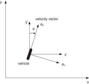
Referring to Figure 3.2, the accelerations in the Cartesian reference (nonrotating) coordinate system can be written in terms of alongtrack acceleration (aa) and crosstrack acceleration (ac)
(3.2-1)
where ![]() . Note that the model is nonlinear, but this does not cause problems for a tracking Kalman filter because the measurement data rate is high and accuracy is good.
. Note that the model is nonlinear, but this does not cause problems for a tracking Kalman filter because the measurement data rate is high and accuracy is good.
FIGURE 3.2: Tank coordinate system.
Then aa and ac are defined as first- or second-order Markov (colored noise) processes with parameters chosen to match different characteristics observed in the ATMT. A preliminary evaluation of model structure was based upon power spectral densities computed by double-differencing the ATMT position data and rotating the computed accelerations into alongtrack and crosstrack components. This showed that both aa and ac had band-pass characteristics, with ac having a much narrower passband than aa. From this observation, the accelerations were modeled as Markov processes with transfer functions of the form
![]()
for first-order or
![]()
for second-order. Third-order models were also tested but ultimately rejected. In state-space notation the complete dynamic model for second-order Markov processes is
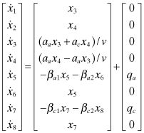
where
(3.2-3)
and
(3.2-4)
![]()
For first-order Markov processes the x7, x8 states are eliminated and derivatives of the acceleration states aa = x5, ac = x6 are
(3.2-5)
![]()
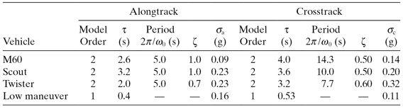
The parameters of these Markov process models were determined using maximum likelihood estimation for each ATMT trial. (Chapter 8 shows how the likelihood function can be computed using outputs of a Kalman filter, and Chapter 11 describes how parameters that maximize the likelihood can be computed.) From the multiple models computed using this approach, four maneuver models that capture the dominant characteristics of data were selected. Table 3.1 summarizes the characteristics of these four maneuver models. The listed “vehicle” is a general description and does not necessarily correspond to tracks from that vehicle. Notice that the standard deviation of the “Twister” ac acceleration is 0.32 g, which is intense maneuvering. In addition to these four models, a “constant velocity” maneuver model (with assumed random walk process noise) was also included for a total of five models used in the adaptive tracking filter.
TABLE 3.1: Reduced Set of Tank Maneuver Models
It should be noted that while these first- and second-order Markov acceleration models work well in tracking Kalman filters, they are not necessarily good long-term simulation models. For example, integration of a first-order Markov process model for acceleration results in infinite velocity. Integration of the above second-order Markov acceleration process has bounded velocity, but does not produce realistic tracks. Hence reduced-order models appropriate for Kalman filters with a short memory may not be accurate models of long-term behavior, particularly for nonlinear systems.
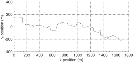
The measurement data available for real-time tracking of the target include observer-to-target azimuth (bearing) angles at a 10-Hz sampling rate, and range measurements every second. The assumed 1 − σ measurement accuracies are 2 m in range and 0.3 milliradians in azimuth. This example is used in Chapter 9 when discussing extended Kalman filters and smoothers, and in Chapter 11 when discussing maximum likelihood parameter identification and multiple-model adaptive trackers. A sample Scout track over a period of about 315 s is shown in Figure 3.3. The average speed when moving is about 7.5 m/s. Unfortunately the position time history data could not be retrieved, so it was necessary to reconstruct the time history from the x-y position data in Figure 3.3. The data were reconstructed using a nonlinear least-squares fitting procedure that included prior knowledge of the average speed. The reconstruction is not perfect because the average speed is closer to 4 m/s, but visually looks very much like Figure 3.3.
FIGURE 3.3: Scout track.
3.2.2 Aircraft Tracking
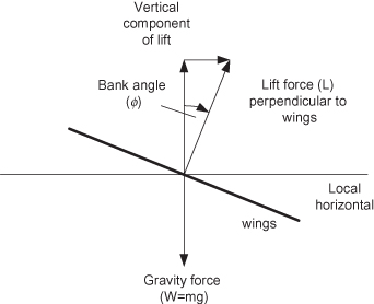
Pilots are taught to maneuver using “coordinated” turns at a fixed rate, to climb/descend at a constant rate, and to use a combination of power and glide path angle changes to alter speed. Coordinated turns are executed so that there is no relative airspeed component in the aircraft lateral direction (parallel to the wings), which minimizes drag and also makes passengers more comfortable because they do not sense any lateral acceleration. Passengers feel that they are being pressed into their seats but, unlike riding in a car when negotiating a curve, are not forced to the outside. Figure 3.4 shows the forces operating in a coordinated turn. To avoid climbing or descending, the vertical component of the lift force must exactly balance the force of gravity, which implies that L cos ϕ = W = mg where m is aircraft mass and g is gravitational acceleration. The lateral (crosstrack) acceleration is ac = (L/m) sin ϕ or ac = g tan ϕ where bank angles of 15 to 30 degrees are usually held constant during the turn. The relationship ac = g tan ϕ is accurate even if moderate climbs or descents are permitted.
FIGURE 3.4: Coordinate turn forces.
Assuming that ac, alongtrack acceleration (aa), and vertical velocity (![]() ) are held constant for periods of time, the following eight-state model of aircraft motion in a fixed Cartesian coordinate frame can be developed.
) are held constant for periods of time, the following eight-state model of aircraft motion in a fixed Cartesian coordinate frame can be developed.
(3.2-6)
where qvz, qac, qaa represent zero mean random process noise that must be included to allow for changes in ac, aa, and ![]() . As shown,
. As shown, ![]() are random walk processes if qvz, qac, qaa are white noise. First-order Markov models (e.g.,
are random walk processes if qvz, qac, qaa are white noise. First-order Markov models (e.g., ![]() ) may seem preferable since
) may seem preferable since ![]() is then bounded rather than growing linearly with time, as for a random walk. However, in practice there is usually little difference in tracking performance of the two models if position measurements (e.g., range, azimuth, and elevation from a ground tracker) are available at intervals of a few seconds. As indicated previously, it is often better to assume that process noise is nominally small or zero, and allow jumps in the
is then bounded rather than growing linearly with time, as for a random walk. However, in practice there is usually little difference in tracking performance of the two models if position measurements (e.g., range, azimuth, and elevation from a ground tracker) are available at intervals of a few seconds. As indicated previously, it is often better to assume that process noise is nominally small or zero, and allow jumps in the ![]() states when changes in acceleration are detected. Methods for implementing this are discussed in Chapter 11.
states when changes in acceleration are detected. Methods for implementing this are discussed in Chapter 11.
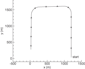
Figure 3.5 shows a simulated aircraft ground track based on the model of equation (3.2-2). The scenario attempts to model a small aircraft within the traffic pattern for an approach to landing. The aircraft is initially located at x = 1200 m, y = 0 m at an altitude of 300 m, and it remains at that height until the final approach leg of the pattern. During and after the final turn, the aircraft descends at a constant rate of 4 to 6 m/s until reaching an altitude of 38 m at the end of the last leg. Aircraft speed is initially 32 m/s but slows to 28.5 m/s after the second turn. Turns are made at bank angles of 25 to 28 degrees. A radar measuring range, azimuth, and elevation every second is located at the origin (0, 0) on the plot. The simulated measurement noise has a 1 − σ magnitude of 1 m in range and 0.2 milliradians for azimuth and elevation. This example is also used in Chapter 9 to demonstrate optimal smoothing.
FIGURE 3.5: Simulated ground track for aircraft approach to landing.
3.3 STRAPDOWN INERTIAL NAVIGATION SYSTEM (INS) ERROR MODEL
Inertial navigation has the advantage that it is independent of external data sources. Inertial navigators may be found on aircraft, missiles, submarines, and ground vehicles. They are sometimes combined with Global Positioning System (GPS) receivers to provide more accurate and robust navigation. Inertial navigators are classified as either gimbaled (stable platform) or strapdown. In a gimbaled system signals from the gyros are used to torque gimbals so that the gyros and accelerometer assemblies remain either fixed in inertial space or locally level. In a strapdown system the gyros and accelerometer assemblies are “strapped” to the vehicle structure and the transformation from the vehicle frame to inertial coordinates is computational. The error characteristics of gimbaled and strapdown INS are very different, but navigation errors in both tend to grow with time (Britting 1971; Grewal and Andrews 2001; Grewal et al. 2001).
INS error behavior is of interest both for system error analysis and because it is used when combining navigation estimates from inertial and GPS systems. Fortunately the error characteristics are well described by linear models. We analyze the strapdown navigator defined in Figure 3.6.
FIGURE 3.6: Strapdown inertial navigator.
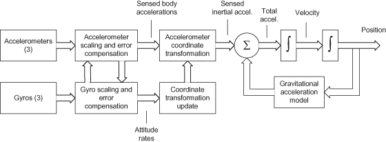
Accelerometers measure the force required to keep a “proof mass” in a reference position within the accelerometer. The proof mass senses the earth’s gravitational force, but does not sense linear acceleration experienced by both the accelerometer body and the proof mass, that is, an accelerometer on an earth satellite subject only to gravitational forces will measure no acceleration. We denote the scaled and compensated output of the three-axis accelerometers—the specific force in accelerometer/gyro coordinates—as fG. The acceleration in computational (inertial) coordinates is calculated by rotating fG to inertial coordinates and adding the computed gravitational acceleration, g(rC), at the inertial position rC:
where ![]() is the rotation (direction cosine) matrix relating the INS body coordinate frame to a fixed, inertial frame.
is the rotation (direction cosine) matrix relating the INS body coordinate frame to a fixed, inertial frame. ![]() is computed knowing the initial orientation of the INS body relative to the inertial coordinates, and then adding all subsequent rotations using gyro outputs. The inertial position is computed by numerically integrating
is computed knowing the initial orientation of the INS body relative to the inertial coordinates, and then adding all subsequent rotations using gyro outputs. The inertial position is computed by numerically integrating ![]() to obtain velocity and then integrating again to obtain inertial position rC.
to obtain velocity and then integrating again to obtain inertial position rC.
The error in measured acceleration is defined as the difference between the measured acceleration ![]() and the true acceleration
and the true acceleration ![]() :
: ![]() . From equation (3.3-1) this is
. From equation (3.3-1) this is
where ![]() is the error in the computed rotation (due to errors in gyro output) and δfG is the error in measured acceleration (without gravity). For purposes of this model, we ignore the last term in equation (3.3-2) as negligible for the problem under consideration (short missile flights).
is the error in the computed rotation (due to errors in gyro output) and δfG is the error in measured acceleration (without gravity). For purposes of this model, we ignore the last term in equation (3.3-2) as negligible for the problem under consideration (short missile flights).
We briefly digress to discuss perturbations in rotation matrices. Perturbations in coordinate transformations from a rotating frame to a fixed (inertial) frame can be represented as
where
(3.3-4)
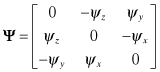
and ψ = [ψx ψy ψz]T are the three infinitesimal rotation angles (radians) along the x, y, and z axes that define the rotation from the original to the perturbed (primed) coordinate frame. Equation 3.3-3 can be derived by computing the coordinate projections from the primed to the unprimed system for infinitesimal rotations ψ using the small angle assumptions cos ψ = 1 and sin ψ = ψ; that is, ![]() and
and
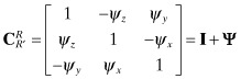
for small ψ. Hence
where we have defined
and ω = [ωx ωy ωz]T is the vector of body rotation rates (radians/s).
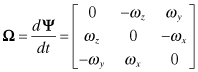
Notice that the error in the direction cosine matrix of equation (3.3-2) can be represented using equation (3.3-3) as
(3.3-7)
![]()
where Ψ is the skew-symmetric matrix defining the “tilt error” in rotation angles. Hence
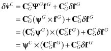
where
| ΨGfG | = ψG × fG (from definitions above), |
| ψG | is the vector of gyro tilt errors as measured in the gyro coordinate system, |
| is the vector of gyro tilt errors in the computational coordinate system, and × denotes vector cross-product. |
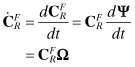
Gyroscopes used for strapdown navigation systems measure instantaneous body angular rates ωG rather than angles. Thus the INS must integrate the angular rates to compute the ![]() rotation. From equation (3.3-5),
rotation. From equation (3.3-5),
(3.3-9)
![]()
with Ω defined in equation (3.3-6). Since ![]() in equation (3.3-8) is defined using
in equation (3.3-8) is defined using ![]() , the tilt error growth in the computational frame can be obtained by integrating
, the tilt error growth in the computational frame can be obtained by integrating
(3.3-10)
![]()
where ωG is the gyro output.
Gyroscope designs are varied (e.g., momentum wheels, Coriolis effect, torsion resonance, ring laser, fiber-optic, etc.), but they all tend to have similar error mechanisms. Specific error sources include biases, scale factor errors (SFEs), drift, input-axis misalignments, input/output nonlinearities, acceleration sensitivity, and g-squared sensitivity. Accelerometer error sources include biases, SFEs, drift, g-squared sensitivity, cross-axis coupling, centrifugal acceleration effects, and angular acceleration sensitivity. Detailed INS error models may include hundreds of error parameters, but we define a 27-state reduced-order model as
where
| δr | is the error in computed inertial position, |
| δv | is the error in computed inertial velocity, |
| ψC | is the tilt error of the gyro/accelerometer computational frame, |
| is the transformation from the gyro to guidance computational (inertial) frame, | |
| fG | is the acceleration expressed in the gyro frame, |
| δα | is the total accelerometer error, |
| ωG | is the angular rate of the gyro-to-computational frame expressed in the gyro frame, |
| δβ | is the total gyro error. |
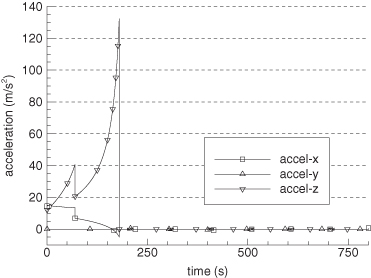
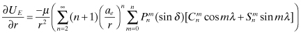
δα and δβ are the sum of several other terms. Table 3.2 lists the 27 error model states, assumed state initial uncertainty and process noise power spectral densities (PSD) for a specific missile test system. Random process noise is assumed to drive only velocity and tilt, and the assumed values integrate to 0.5 mm/s (velocity) and 1.55 arc-sec (tilt) 1 − σ in 10 min. The measurements consist of position error in each channel (δx,δy,δz) with a measurement error of 0.61 mm 1 − σ. (This extreme high accuracy is only obtained with special test instrumentation, and is not typical for standard measurement systems such as GPS.) Measurements were taken every 10 s during a missile flight of 790 s to give a total of 237 scalar measurements. Note that the dynamic error equations require input of specific force and body rates versus time. A two-stage missile booster with burn times of 70 and 110 s, respectively, flown with a 5 degrees offset between the thrust vector and velocity vector, was simulated. The peak trajectory altitude was approximately 2900 km at 1200 s of flight. After the boost phase, the simulated payload maneuvered every 100 s where the specific force was one cycle of a sinusoid (0.07 g maximum) with a period of 15 s. Figure 3.7 shows the simulated Earth-Centered Inertial (ECI) specific force (acceleration less gravity) for the simulated flight. The acceleration due to booster staging is apparent, but acceleration due to bus maneuvers (0.7 m/s2 peak) is not evident at this scale.
TABLE 3.2: Inertial Navigator States and Initial Uncertainty
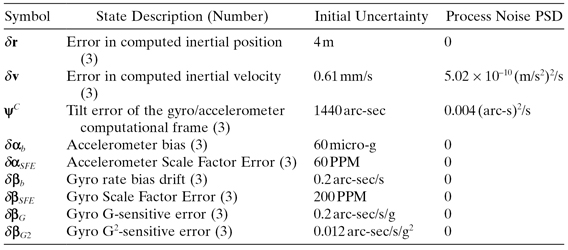
FIGURE 3.7: Simulated ECI missile acceleration.
The dynamics model has the form
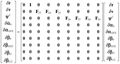
where all partitions are 3 × 3 and are computed according to equation (3.3-11) using ![]() , fG, and ωG evaluated along the reference trajectory:
, fG, and ωG evaluated along the reference trajectory:
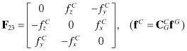
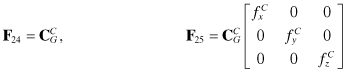
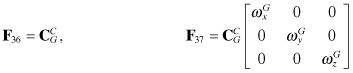
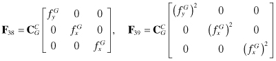
The somewhat strange use of fG components for F38 and F39 is due to the definitions of the gyro frame (x = along the velocity vector, y = r × x, and z = x × y) and the gyro alignment. Not shown in these equations are unit conversions that may be necessary if accelerometer and gyro errors have units different from those of velocity and tilt.
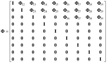
In this particular problem the differential equations are integrated at a 0.2 s interval with 10 s between measurements. Accelerometer specific force and gyro angular rates are updated at 0.2 s intervals and the state equations (eq. 3.3-11) are integrated using a second-order Taylor series. Because of the very high integration rate and slow dynamics, the state transition matrix is computed as Φ = I + FT, and QD is assumed to be diagonal over a 0.2-s interval. Accuracy is more important when computing measurement residuals than when propagating the error covariance using Φ and QD.
By including additional terms of the Taylor series, it can be shown that Φ has the form of equation (3.3-12). Notice that Φ retains much of the sparse structure of F, but fills in additional terms in the upper triangle. The type of sparse structure depends upon the ordering of states. Filter code execution can often be made more efficient if biases are placed at the end of the state vector and integral states, such as position, at the beginning. In this case QD will only have nonzero elements in the upper left 9 by 9 block.
(3.3-12)
This INS example is used in Chapter 11 to demonstrate how a jump detection algorithm is added to a Kalman filter. The simulated jumps are listed in Table 3.3. The example is also used in Chapter 9 to demonstrate Kalman filter error analysis, and in Chapter 10 to compare the accuracy of different Kalman filter implementations.
TABLE 3.3: Simulated INS Jumps
| Simulation Jump Time (s) | Jump Parameter | Jump Magnitude |
| 25 | y-gyro SFE | −60 PPM |
| 50 | y-gyro G-sensitive error | +0.10 arc-sec/G |
| 100 | z-gyro rate bias drift | −0.10 arc-sec/s |
| 120 | x-accelerometer SFE | +1.0 PPM |
| 400 | y-accelerometer bias | −4 micro-G |
3.4 SPACECRAFT ORBIT DETERMINATION (OD)
Dynamics of an earth satellite are of interest (1) for historical reasons, (2) because it is still an active application area, and (3) because the OD problem demonstrates a number of interesting estimation issues involving nonlinear models and poor observability.
Satellite orbital dynamics are usually modeled in an Earth-Centered Inertial (ECI) coordinate frame. The ECI x-y plane is the earth’s equatorial plane, and the z-axis is the earth’s spin vector. The x-axis is defined so that it passes through the intersection (vernal equinox) of the earth’s equatorial plane and the ecliptic plane (the plane containing the mean orbit of the earth around the sun). Due to precession and nutation of the earth’s spin axis, ECI frames must be specified at some epoch time, and assumptions about precession and nutation must also be specified. The two most commonly used ECI frames are the J2000 and true-of-date (TOD) frames. The J2000 frame uses the mean (ignoring nutation) equator and equinox of Universal Time Coordinated (UTC) noon on January 1, 2000, called J2000.0. The TOD frame uses both earth precession and nutation at the specified epoch when calculating the ECI orientation. Most orbital integration is performed in the J2000 frame because TOD frames are slowly rotating and thus not truly inertial. See Seidelmann (2006), Tapley et al. (2004), Vallado and McClain (2001), Wertz (1978), Escobal (1976), and GTDS Mathematical Theory (1989) for more information on orbital coordinate systems and orbit definitions.
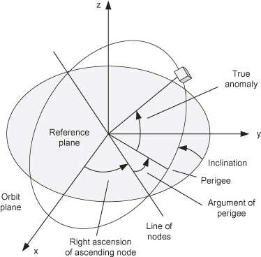
Spacecraft orbits are defined using six orbital parameters. Orbits are often specified using Kepler elements (Fig. 3.8) that define the orientation of an orbital ellipse and the position in the ellipse:
1. Semimajor axis of ellipse
2. Eccentricity of ellipse
3. Inclination of ellipse with respect to reference plane (earth equatorial plane for a geocentric orbit)
4. Right ascension of ascending node: the central angle in the reference plane, measured from the x-axis, at which the ellipse intersects the reference plane with the satellite moving in a northerly direction
5. Argument of perigee: the central angle from the ascending node to the perigee of the ellipse measured in the direction of motion
6. Mean anomaly: the central angle from perigee to the current orbital position at the given time, but defined as if the orbit is circular. Mean anomaly is not a physical angle. It is measured assuming that the mean angular rate is constant rather than varying with radial distance. True anomaly is the central angle from perigee to ellipse focus to the current orbital position, but because the angular rate changes throughout the orbit, it is not directly useful for modeling orbit propagation.
FIGURE 3.8: Kepler orbital elements.
Kepler elements are convenient for understanding elliptical orbits. Because the first five parameters are constant for a two-body orbit (one in which the gravitational attraction between the two bodies is the only force acting on the satellite), calculation of the inertial position as a function of time is relatively easy. Since the mean anomaly changes at a constant mean orbital motion rate, the change in mean anomaly at any given time is simply mean motion multiplied by the time interval from epoch. Unfortunately, real satellite orbits are affected by forces other than just central gravitation, so propagation for a real orbit is more difficult. Furthermore, Kepler elements are indeterminate for circular or zero-inclination orbits. An alternate representation, equinoctial elements, avoids this problem by using two-parameter inclination and eccentricity vectors, and replacing mean anomaly with mean longitude (Bate et al. 1971; Vallado and McClain 2001). For circular or zero-inclination orbits, the vector elements are simply zero. However, propagation of equinoctial elements for real orbits is also nontrivial. For that reason, six ECI Cartesian position and velocity elements are usually used for numerical integration of orbits.
Using ECI Cartesian elements r and v, the orbital dynamics for a constant mass spacecraft are
where f is the total ECI external force (vector) acting on the spacecraft and m is the spacecraft mass. The total external force can be represented as
(3.4-2)
![]()
where
| fE | is the force due to the gravitational potential of the earth, |
| fG | is the differential force due to the gravitational potential of the sun, moon, and planets, |
| fS | is the force due to solar radiation pressure and other radiation, |
| fD | is the force due to aerodynamic drag, |
| fT | is the force due to spacecraft thrusting. |
Note that when the spacecraft is generating thrust, mass changes, so the second line of equation (3.4-1) must be modified. We now examine each of the force components, or in the case of gravitational attractions, compute the acceleration directly.
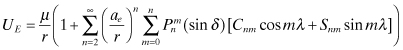
3.4.1 Geopotential Forces
The earth’s gravitational potential UE at a point r, δ, λ outside the earth is defined by the Laplacian ∇2U = 0. The solution can be expressed as a spherical harmonic expansion in Earth-Centered-Fixed (ECF) coordinates:
where
| μ | = gravitational constant |
| r | = geocentric distance |
| ae | = mean equatorial radius of the earth |
| = associated Legendre function of the first kind of degree n and order m | |
| δ | = geocentric declination (geocentric latitude) |
| λ | = geocentric east longitude |
| Cnm, Snm | = harmonic coefficients of degree n and order m |
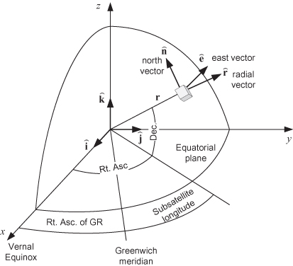
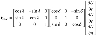
In practice the above series for n is truncated at an order sufficient to achieve the desired accuracy. The n = 1 term in equation (3.4-3) does not normally contribute if the coordinate system origin is at the center of mass. Note that equation (3.4-3) uses geocentric latitude (declination) and longitude as defined in Figure 3.9: the x- and y-axes are in the equatorial plane, the x-axis on the Greenwich meridian, and the z-axis is the earth spin axis. To be rigorously correct, the ECF system should include polar motion, but the approximately two microradian polar motion shift is often ignored as having negligible effect on the computed gravitational field.
FIGURE 3.9: Local horizon coordinate system for geopotential.
Starting with the spacecraft position vector in J2000 coordinates, the position in ECF coordinates is computed using precession/nutation rotations and a rotation for Greenwich Hour Angle:
(3.4-4)
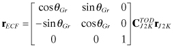
where θGr is the right ascension of Greenwich at the given time and ![]() is the rotation matrix from the J2000 coordinate system (mean-equator and mean-equinox of January 1, 2000 noon) to TOD coordinates (true-equator and true-equinox of current date).
is the rotation matrix from the J2000 coordinate system (mean-equator and mean-equinox of January 1, 2000 noon) to TOD coordinates (true-equator and true-equinox of current date). ![]() models precession and nutation of the earth’s spin axis (Tapley et al. 2004; Seidelmann 2006). The right ascension of the satellite is the sum of longitude and Greenwich Hour Angle:
models precession and nutation of the earth’s spin axis (Tapley et al. 2004; Seidelmann 2006). The right ascension of the satellite is the sum of longitude and Greenwich Hour Angle:
(3.4-5)
![]()
Then the geocentric latitude and longitude can be computed from the ECF coordinates as
(3.4-6)
although it is not necessary to work directly with these angles (all computations involve trigonometric functions).
The inertial acceleration vector due to earth gravitation in ECF coordinates is computed using the gradient of the potential function, that is,
(3.4-7)
![]()
The partial derivatives of the potential with respect to radius, longitude, and declination (geocentric latitude) are, respectively,
(3.4-9)
![]()
The following recursive formulae are used for the Legendre functions:
(3.4-11)
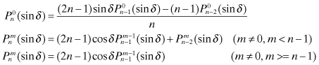
where
(3.4-12)
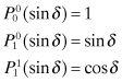
and
![]()
![]()
![]()
The μ, ae, ![]() , and
, and ![]() coefficients define the gravitational model. Different geopotential fields have been developed using tracking of thousands of satellite arcs, along with other types of measurements. The geopotential field model used by the U.S. Department of Defense and for the GPS is the World Geodetic System 84 (WGS84; Department of Defense World Geodetic System 2004). The latest revision of WGS84 is called the Earth Gravitational Model 1996 (EGM96) and includes revisions through 2004. In this system, μ = 398600.4418 km3/s2, ae = 6378.1370 km, and the spherical harmonic coefficients are computed up to degree and order 360.
coefficients define the gravitational model. Different geopotential fields have been developed using tracking of thousands of satellite arcs, along with other types of measurements. The geopotential field model used by the U.S. Department of Defense and for the GPS is the World Geodetic System 84 (WGS84; Department of Defense World Geodetic System 2004). The latest revision of WGS84 is called the Earth Gravitational Model 1996 (EGM96) and includes revisions through 2004. In this system, μ = 398600.4418 km3/s2, ae = 6378.1370 km, and the spherical harmonic coefficients are computed up to degree and order 360.
Derivatives of the potential from equations (3.4-8) to (3.4-10) are then expressed as gradients in the radial, eastward, and northward directions:
(3.4-13)
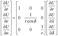
where ![]() . These local East and North unit vectors are defined from Figure 3.9 in ECI TOD coordinates as:
. These local East and North unit vectors are defined from Figure 3.9 in ECI TOD coordinates as:
(3.4-14)
![]()
(3.4-15)
![]()
(3.4-16)
![]()
Then the inertial acceleration in ECI TOD coordinates is obtained using rotations for latitude (declination) and longitude:
where
![]()
![]()
Note that equation (3.4-17) is the inertial acceleration due to the geopotential defined in the ECF system. (It is not acceleration with respect to the rotating ECF coordinate system.) It must be rotated into the TOD geocentric inertial coordinate system using the Greenwich Hour Angle:
(3.4-18)
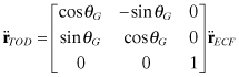
Alternately the two rotations for longitude and GHA can be combined into a single rotation.
Finally, ![]() is rotated to the J2000 ECI system as
is rotated to the J2000 ECI system as
(3.4-19)
![]()
using the precession/nutation transformation.
Another gravitational effect included in high-accuracy orbit models is due to the deformation of the earth caused by sun and moon gravitation. This solid earth tide effect can be 30 cm vertically at some locations, and the bulge lags behind the actual sun and moon position. The tide effect is not only important for modeling ground tracking station locations, but it also has a significant effect on the geopotential field. Solid earth tide models are discussed in Tapley et al. (2004), McCarthy (1996), and McCarthy and Petit 2004). Ocean tides also have a small effect on the geopotential field, and they may be modeled.
Finally, the general relativistic effect on time scales due to earth’s gravitational field is sometimes modeled when working with systems that are accurate to centimeter levels, such as the GPS (Parkinson and Spilker 1996; McCarthy and Petit 2004; Tapley et al. 2004).
3.4.2 Other Gravitational Attractions
The total potential acting on a satellite can be written as:
(3.4-20)
![]()
where UG is the disturbing function due to the gravitational attractions of other bodies. This is written as:
(3.4-21)
![]()
where
| μi | = μ(mi/me) |
| mi | = mass of the ith body |
| me | = mass of the earth |
| ri | = geocentric position vector of the ith body |
The resulting perturbing acceleration due to UG is
(3.4-22)
![]()
In words, the perturbing effect on a satellite due to gravitational attractions is the difference of direct attractions of the bodies on the satellite, and the attractions of the bodies on the earth. The sun and moon are the most significant perturbing bodies and are often the only ones modeled.
3.4.3 Solar Radiation Pressure
Solar radiation pressure acting on a spacecraft is usually computed using one of two methods. If the spacecraft is nearly spherical or has large movable solar panels that are continually pointed nearly normal to the sun, it is commonly assumed that the solar radiation force can be computed as if the spacecraft absorbs all photon momentum without regard for the orientation of the spacecraft with respect to the sun. This is sometimes referred to as the ballistic or cannonball model. The force vector is computed as
(3.4-23)
![]()
where
| v | = illumination factor (0 to 1) |
| A | = effective cross-sectional area (m2) |
| Fe | = mean solar flux at 1AU (∼1358 W/m2) |
| c | = speed of light (m/s) |
| AU | = 1 Astronomical Unit (1.49597870 × 10¹¹ m) |
| rsc | − rsun = sun-to-spacecraft vector (m) |
| r | = |
| Cr | = radiation pressure coefficient (nominally 1.0). |
The illumination factor v is equal to 1 except during eclipse (v = 0 when in a full eclipse).
Alternately the total solar radiation pressure force can be computed by modeling each external structure on the spacecraft and summing the force vectors for each structure. For a plate, the force due to direct solar radiation pressure is typically modeled as a combination of diffuse reflection, specular reflection, and absorption:
(3.4-24)
![]()
where
| rpl | − rsun = sun-to-plate vector (m) |
| r | = |
| = unit normal to plate surface | |
| Cd | = diffuse reflection coefficient (0 to 1) |
| Cs | = specular reflection coefficient (0 to 1) |
The calculation for other structures such as cylinders or cones is similar but requires integration of the differential force over the entire surface. Also, shadowing of one structure by another may be included in the calculation of v.
To determine the illumination factor for eclipses of the sun by the earth, first define
(3.4-25)
where rsc is the geocentric position vector of the spacecraft. If β > π/2, the spacecraft is on the same side of the earth as the sun and no eclipse can occur. Hence v = 1. Otherwise an eclipse is possible. In that case, calculate
(3.4-26)
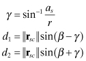
where as is the radius of the sun. If d2 ≤ ae where ae is the radius of the earth, then the spacecraft is inside the umbra and v = 0. If d1 ≥ ae the spacecraft is outside the penumbra and v = 1. If d1 < ae and d2 > ae, the eclipse is partial and v ≅ (d2 − ae)/(d2 − d1). Similar equations can be used for sun eclipses by the moon if the vectors and radius are defined accordingly.
The transition from penumbra to umbra only lasts about 2.1 min for geosynchronous orbits and much less for low altitude orbits so it may not be necessary to model the penumbra/umbra transition in the orbit integration. An alternative just tests whether ![]() rsc
rsc![]() sin β < ae to determine when the spacecraft is in eclipse (v = 0).
sin β < ae to determine when the spacecraft is in eclipse (v = 0).
In some high-accuracy cases, the pressure from solar radiation diffusively reflected from the earth or moon may also be included in the calculation of total radiation force. The average albedo of the earth is about 30%, so the effect can be important. Also, the force due to energy radiated from the spacecraft (from antennas or instrument coolers) may sometimes be included.
3.4.4 Aerodynamic Drag
For spacecraft that descend into the earth’s atmosphere (below about 2500 km altitude), atmospheric drag may be a significant perturbing force. If it is assumed that all aerodynamic forces are along the relative velocity vector (no transverse aerodynamic forces), the drag force can be modeled as
(3.4-27)
![]()
where
| vr | = v − ωer is the relative velocity vector (m/s) between spacecraft and earth (ωe is the earth rotation rate), |
| ρ | is the atmospheric density (kg/m3) at the satellite’s position |
| CD | is the drag coefficient (usually between 1 and 2) |
As with solar radiation pressure, drag and lift forces can be modeled taking into account the separate shapes of structures attached to the spacecraft, if it is not nearly spherical.
Calculation of ρ at the satellite position is one source of error when computing the drag force. Most atmospheric density models are derived from either the Harris-Priester model or a version of the Jacchia-Roberts models. The Harris-Priester model is a time-dependent diffusion model based on the assumption that the nominal density profile with altitude is fixed, but a diurnal bulge in density lags behind the sun position by 30 degrees. It is a relatively simple model that is easy to implement. The Jacchia-Roberts models are time-invariant, but involve many terms. The Mass Spectrometer and Incoherent Scatter Radar (MSIS) Neutral Atmosphere Empirical Model NRLMSISE-00 (Picone et al. 1997) was derived using satellite and rocket data. For further information see GTDS Mathematical Theory (1989), Wertz (1978), Tapley et al. (2004), and the NASA Goddard Space Flight Center web site (ftp://nssdcftp.gsfc.nasa.gov/models/atmospheric/).
3.4.5 Thrust Forces
Orbital maneuvers or momentum-dumping maneuvers executed using low-thrust chemical thrusters generally involve short firing times. Hence they are usually treated as an impulsive velocity change (Δv) where orbit propagation proceeds to the time of the maneuver, the Δv is added to velocity, and orbit propagation proceeds. However, orbit injection maneuvers and maneuvers conducted using very low thrust ion propulsion thrusters are conducted over an extended period of time. Hence these maneuvers are modeled by integrating the thrust force
(3.4-28)
![]()
where ft_body is the thrust force in body coordinates and ![]() is the rotation from spacecraft body to ECI coordinates. For moderate to high-thrust orbit injection maneuvers, the change in mass during the maneuver should also be modeled. That is,
is the rotation from spacecraft body to ECI coordinates. For moderate to high-thrust orbit injection maneuvers, the change in mass during the maneuver should also be modeled. That is, ![]() where Isp is the specific impulse of the thruster, and m should be carried as a seventh dynamic state in the orbital model.
where Isp is the specific impulse of the thruster, and m should be carried as a seventh dynamic state in the orbital model.
In many cases it is also important to model impingement of the chemical thruster plume on solar arrays or other spacecraft structures. Chemical thrusters can have plume half-widths of 20–25 degrees, and the impingement forces and torques can be 1% to 2% of the total maneuver.
3.4.6 Earth Motion
Many internal computations in orbit generation or OD software require the relative position between the spacecraft and fixed points on the earth at specified times. Unfortunately the rotational motion of the earth is not constant: the spin axis changes slightly with time and the rotation rate (and thus earth-referenced time) also changes. The offset between “earth rotation time” and “atomic time” (actually Terrestial Time) and the “polar motion” offset of the spin axis are determined using astronomical and GPS measurements (McCarthy 1996; McCarthy and Petit 2004; Seidelmann 2006). The International Earth Rotation and Reference Systems Service (IERS) calculates these changes and issues updates weekly (http://maia.
usno.navy.mil/). In addition to these slow changes, occasional 1 s jumps are added or subtracted to UTC time so that the discrepancy between actual earth rotation and UTC time is maintained less than 0.9 s. These leap second jumps, when they occur, are applied at midnight on June 30 or December 31 of the year. IERS Bulletins also list these leap seconds.
The transformation from J2000 coordinates to ECF coordinates involves four separate transformations:
(3.4-29)
![]()
where
| is the direction cosine rotation for earth precession from J2000.0 to the specified date/time, | |
| is the rotation for earth nutation from J2000.0 to the specified date/time, | |
| is the rotation for Greenwich Apparent Sidereal Time (which is actually an angle θ) at the specified date/time. θ depends on data in IERS Bulletins. | |
| is the rotation for polar motion at the specified date/time (xp and yp are defined in IERS bulletins). |
The rotation from ECF to J2000 coordinates is the transpose of the above. More information on earth modeling can be found in Seidelmann (2006), Tapley et al. (2004), McCarthy and Petit (2004).
3.4.7 Numerical Integration and Computation of Φ
The nonlinear differential equations defined by equation (3.4-1) must be integrated to obtain the position and velocity at a specified time. Analytic methods have been developed to approximately integrate the equations using different assumptions about applied forces, but these methods are seldom used today in operational software. In the 1960s and for several decades later, predictor-corrector ODE integration algorithms were used for most high-precision satellite orbital dynamic computations. Multistep methods, such as predictor-corrector, are difficult to use because they require single-step methods to start the integration, and they are inflexible when a change in the integration step size is required. Higher order Runge-Kutta integration (a single-step method) was also sometimes used. Today the Bulirsch-Stoer extrapolation and Runge-Kutta methods are the most popular, where Bulirsch-Stoer is generally regarded as more accurate (Press et al. 2007, Chapter 17). When the force model is conservative (does not depend on velocity, which excludes the drag model), computations of the Bulirsch-Stoer method can be reduced by nearly 50% when using Stoermer’s rule (Press et al. 2007, Section 17.4).
The differential equations defining orbit propagation are nonlinear, but most OD algorithms require computation of a state transition matrix Φ for a linear perturbation model. The earliest OD software computed Φ by integrating the variational equations—the partial derivatives of equation (3.4-1) with respect to position and velocity and any other parameters of the model that are estimated in the OD; that is, ![]() . This required thousands of lines-of-code to compute the partial derivatives, and greatly limited the flexibility of the software. Many new OD programs either compute F using numerical partial derivatives and then integrate
. This required thousands of lines-of-code to compute the partial derivatives, and greatly limited the flexibility of the software. Many new OD programs either compute F using numerical partial derivatives and then integrate ![]() , or directly compute Φ using numeric partials as described in Section 2.3.1. The generic structure of Φ used in OD is
, or directly compute Φ using numeric partials as described in Section 2.3.1. The generic structure of Φ used in OD is
(3.4-30)
where all matrix partitions are either 3 × 3 or 3 × p, and β is a p-element vector of force model constants—such as Cr, CD, gravity field coefficients or thrust parameters—included in the OD. The ∂v(t + T)/∂r(t) partition will be zero if the perigee altitude is high enough (e.g., >2500 km) so that drag forces are zero. If no other forces depend on velocity, the force model is conservative.
Another approach to computing Φ uses equinoctial elements, rather than Cartesian position/velocity, as states in the OD. The equinoctial elements directly model the dominant force acting on the spacecraft (earth central gravity) so the effect of the other forces (gravity field, sun/moon gravity, solar radiation, drag, thrust) is a small perturbation. Somewhat surprisingly, the upper left 6 × 6 partition of Φ for an equinoctial element state can be computed accurately for some high-altitude satellites by just modeling the spherical harmonic gravity field to degree two; that is, the ![]() (also called J2 when normalized) coefficient with
(also called J2 when normalized) coefficient with ![]() are the only coefficients included. Derivation of the 6 × 6 Φ partition is nontrivial (see Koskela 1967; Escobal 1976; or GOES N-Q OATS SMM 2007, Section 6.3.2.2) but not difficult to compute. A similar approach can also be applied to compute the partitions of Φ that model sensitivity of equinoctial elements with respect to Cr, CD, and thrust parameters.
are the only coefficients included. Derivation of the 6 × 6 Φ partition is nontrivial (see Koskela 1967; Escobal 1976; or GOES N-Q OATS SMM 2007, Section 6.3.2.2) but not difficult to compute. A similar approach can also be applied to compute the partitions of Φ that model sensitivity of equinoctial elements with respect to Cr, CD, and thrust parameters.
Most OD is performed using batch least-squares methods since deterministic orbital force models are quite accurate for many satellites. However, it is not possible to model all forces perfectly (particularly for satellites within the earth’s atmosphere), and in some high-accuracy cases it is preferable to use a Kalman filter that treats errors in the dynamic model as process noise. Kalman filters are used in GPS satellite OD (Parkinson and Spilker 1996; Misra and Enge 2001; Kaplan and Hegarty 2006,) and for some LEO spacecraft (Gibbs 1978, 1979). Filters often model process acceleration errors in alongtrack, crosstrack, and radial directions as independent white noise (random walk in velocity) or first-order Markov processes. For the first-order Markov model:
(3.4-31)
where
| is the ECI acceleration at time t, | |
| f(r,v) | is the force model for the gravity field, sun/moon/planet gravity, solar radiation, drag, and thrust, |
| is the rotation from alongtrack, crosstrack, and radial coordinates to ECI (a different transformation could also be used if model errors are more likely to appear in a different direction), | |
| ap(t) | is the vector of alongtrack, crosstrack, and radial accelerations at time t, |
| qa(t), qc(t), qr(t) | are the alongtrack, crosstrack, and radial random process noise at time t, |
| τa, τc, τr | are the alongtrack, crosstrack, and radial time constants. |
In this model the three components of ap(t) are included as states in the Kalman filter, and the discrete process noise covariance QD is computed as described in Chapter 2. For a random walk velocity model, white noise is rotated to ECI coordinates and directly added to the velocity rate (![]() ) so no acceleration states are included in the filter. Process noise may also be used to model thrust acceleration errors during long maneuvers.
) so no acceleration states are included in the filter. Process noise may also be used to model thrust acceleration errors during long maneuvers.
3.4.8 Measurements
The measurements typically used in OD include ground-based range, range rate and tracking angles, satellite-to-satellite range and range rate (usually multi-link to ground), satellite measured angles to ground objects, and GPS pseudo-ranges. Other variants on these basic types are also possible. Recall from Section 1.2 that least-squares and Kalman estimation compare actual measurements with model-computed measurements, although the model-computed measurements may be zero in linear least squares.
We now derive the equations for these measurement types given satellite positions and velocity, and ground location.
3.4.8.1 Ground-Based Range, Range Rate, Integrated Range Rate, and Tracking Angles
The basic equations for range and range rate measurements were presented in Example 2.4. Ground tracking of a satellite usually involves measuring either the two-way (uplink and downlink) time delay or the two-way phase changes if continuous tones are used for the measurement. Because the distances and velocities are great, and transmitters and receivers are both moving in an inertial frame, it cannot be assumed that the average two-way transit time or phase change can be treated as a measure of the geometric distance between ground observer and satellite at the received measurement time. For example, the distance to a geosynchronous satellite from a ground station may be 37,000 km, and the satellite velocity is about 3 km/s. Using the speed of light in a vacuum (c = 299792.458 km/s), the signal transit time is calculated as 0.123 s, and the satellite will have moved about 369 m in that time. A crude procedure for calculating the downlink range is as follows:
1. Calculate ground location and satellite position/velocity in ECI coordinates at the ground receive time t.
2.
Calculate an approximate ground-satellite range (r′ = ![]() rgnd(t) − rsc(t)
rgnd(t) − rsc(t)![]() ) and the transit time, Δt = r′/c.
) and the transit time, Δt = r′/c.
3. Recalculate satellite position and velocity at t − Δt.
4. Recalculate ground-satellite range using the satellite position at t − Δt.
Unfortunately the final range will still not be accurate, and it is necessary to repeat this procedure several times until the computed range does not change. A better method expands the equation for range-squared at different ground/satellite times,
![]()
in a second-order Taylor series,
![]()
and then solves the quadratic equation for Δt assuming that the satellite acceleration is only due to earth central-body gravity (![]() ). This method is accurate to better than 3 × 10⁻⁶ m for geosynchronous satellites. The same procedure is repeated for the uplink from the ground to the satellite. Range rate measurements can be included as part of the same calculation.
). This method is accurate to better than 3 × 10⁻⁶ m for geosynchronous satellites. The same procedure is repeated for the uplink from the ground to the satellite. Range rate measurements can be included as part of the same calculation.
Topocentric elevation and azimuth angles are computed from the position difference vector rgnd(t) − rsc(t − Δt) rotated into the local level system (z = local vertical, y in a northerly direction in the plane normal to z, and x = z × y). These angles are often available from tracking antennas, but they should be used with caution. Antennas used for transmitting/receiving telemetry data may use an angle-tracking control loop that attempts to model the orbit of the satellite. The error characteristics of this angle data are not ideal for OD because the angles may be highly correlated in time and may change rapidly as the tracking algorithm updates the model. The accuracy may also be inadequate for good OD. Check the data before using.
Range, range rate, and angle measurements from the ground to a satellite are influenced by tropospheric and ionospheric effects. Since the index of refraction in the troposphere is greater than 1.0, the effective group propagation speed is less than c and range measurements computed as Δt/c will have a positive bias. That bias is a minimum at zenith (because of the shorter path through the troposphere) and it increases approximately as 1/(sin E + 0.026) with decreasing elevation E. Because of this error, tracking is usually terminated below an elevation cutoff in the range of 5 to 15 degrees. Likewise the propagation speed through the ionosphere is also less than c and the range error is a minimum at zenith. Because the ionosphere is a dispersive medium, the delay varies approximately as the inverse squared power of carrier frequency; that is, it is much greater at L-band than C-band frequencies. This dependence on frequency is used in the two-frequency P-code GPS system to calculate the ionospheric effect and remove it. In addition to group delay effects, the change in index of refraction along the signal path bends the ray, and thus angles measurements are biased. Again the effect varies with elevation. Other delays that alter range measurements include satellite transponder and ground link delays (possibly time-varying).
Angular measurements of satellites can be also be obtained by optically comparing the observed satellite position with that of background stars. Measurement processing is complicated by the need to account for proper motion, parallax, annual aberration, and planetary aberration of the stars (Seidelmann 2006). Angular measurements are also affected by equipment biases and planetary aberration.
All these effects should be modeled when processing the measurements. There are two ways in which this can be done: model the errors when generating a “calculated measurement” to be compared with the actual measurement in the OD, or approximately calculate the error and correct the measurement before processing in OD. Both approaches are used, but the “preprocessing” method has the advantage that the computations are not included when calculating OD partial derivatives. Measurement preprocessing is routinely used in many systems because it also allows for editing of anomalous measurements prior to processing in the estimation algorithm. It is sometimes difficult to detect anomalous measurements prior to updating the state estimate (particularly when the initial state estimate is poorly known), so editing done during preprocessing can make the system significantly more robust. Sometimes this is done by fitting a linear or quadratic model to a short time series of measurements and editing measurements that deviate more than n-sigma from the curve fit. This works best when the measurement sampling rate is much higher than the highest frequencies at which the dynamic system responds. For these high sampling rate cases, it can be advantageous to compute an “average” measurement over a time window from the curve fit, and use that measurement in the OD. This reduces OD computations and allows applying greater weight to “averaged” measurements than raw measurements because the random errors are smaller. This approach is discussed again in later chapters.
3.4.8.2 Satellite-to-Satellite Range and Range Rate
Satellite-to-satellite range and range rate measurements are modeled similarly to ground-based measurements, except that the motion of both satellites must be modeled. Atmospheric effects can be ignored if both satellites are above the atmosphere and the ray path does not pass through the atmosphere.
3.4.8.3 Satellite Measured Angles to Ground Points or Stars
Angles from ground points (including the horizon) to satellites are modeled using the inertial vector from the ground to the spacecraft, taking into account the transit time of the ray. Then the vector is rotated from inertial to spacecraft coordinate system and angles are computed as projections on the spacecraft axes. The angle measurements are also affected by planetary aberration, tropospheric refraction, and errors in computing the attitude of the spacecraft. Measured angles to stars (e.g., from a star tracker) are modeled similarly using the inertial coordinates of the stars. Additional error effects include parallax, proper motion of the stars, annual aberration, and planetary aberration. Star measurements provide more information on spacecraft attitude than orbit.
3.4.8.4 GPS Pseudo-Range and Carrier Phase
Pseudo-range (PR) and accumulated delta-range (ADR) or carrier phase measurements obtained using GPS signals are similar to range and integrated range rate measurements, but include a large bias and drift that are due to the unknown time and frequency errors of the receiver. The ADR measurements are less noisy than PR, but both contain tropospheric and ionospheric delay. The PR-ADR difference is not influenced by tropospheric delay modeling error, but contains a satellite-receiver pass-dependent bias. The navigation message transmitted with the GPS signal provides accurate information on the ephemeris and clock errors of the GPS satellites, and also has information allowing single-frequency users to model the ionospheric delay. A typical terrestrial GPS navigator must simultaneously receive signals from at least four GPS satellites in order to uniquely calculate the three components of its position and its local clock error. For satellite receivers, it is not necessary to simultaneously receive four GPS signals and calculate position, since this can be done in the OD from GPS signals received over a period of time. This is convenient because the transmitting antenna of the GPS satellites is designed to only provide earth-coverage, so satellites at a higher altitude (>20.2 km) will receive signals when the signal path is near the earth’s edge. Most receivers in geosynchronous orbits can also receive signals transmitted from GPS antenna sidelobes. Sidelobe signals from six or seven GPS satellites can usually be received, but future GPS antenna designs may not retain signal strength in the sidelobes.
Test Case #1: Low Earth Orbit (LEO) Satellite
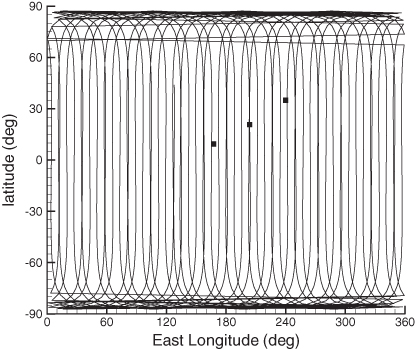
Two cases are used for examples in Chapters 6 and 7. The model for the first case is a CHAllenging Mini-satellite Payload (CHAMP) three-axis stabilized earth-pointing spacecraft. It is designed to precisely measure the earth’s gravity field using GPS and accelerometer sensors, and to measure characteristics of the upper atmosphere. The nearly circular orbit has an altitude of 350 km (92-min period) and 87.2 degrees inclination. At this altitude CHAMP is well within the earth’s atmosphere and is significantly affected by atmospheric drag. Either the Harris-Priester or MSIS atmospheric models are used in the example, but this is the largest source of orbit modeling error. The J2000 parameters of the orbit are defined in Table 3.4, and approximate locations of three ground tracking stations are listed in Table 3.5. Figure 3.10 shows the ground track for a 2-day period (2005 days 141 and 142) and the locations of the ground tracking stations.
TABLE 3.4: Case #1 (CHAMP) Simulated Orbit Parameters
| Parameter | Value (J2000 Coordinate Reference) |
| Epoch time | 00:00:00 2008 day 141(UTC) |
| Semimajor axis | 6730.71 km |
| Eccentricity | 0.0012975 |
| Inclination | 87.244 degrees |
| Right ascension of ascending node | 189.425 degrees |
| Argument of perigee | 56.556 degrees |
| Mean anomaly | 75.376 degrees |
| Solar radiation pressure Kp = CpA/m | 0.05 |
| Drag coefficient Kd = CdA/m | 0.00389 |
TABLE 3.5: Case #1 (CHAMP) Simulated Ground Stations
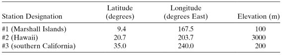
FIGURE 3.10: CHAMP ground track and ground stations.
For this example the orbit is determined using range, azimuth, elevation, and range rate measurements from each station, where the assumed 1 − σ measurement errors are 15 m, 0.5 degrees, 0.4 degrees, and 2.0 m/s, respectively. Simulated range and range rate data is generated every 120 s when the satellite is in view. Measurement bias is ignored.
Test Case #2: Geosynchronous Earth Orbit (GEO) Satellite
This case uses orbit elements appropriate for a geosynchronous spacecraft located at approximately 89.5 degrees west longitude. The orbit parameters are listed in Table 3.6. A ground station located at 37.95 degrees latitude, 75.46 degrees west longitude, and −17 m with respect to the reference ellipsoid measures range to the spacecraft. This scenario is typical for the GOES-13 spacecraft during post launch testing.
TABLE 3.6: Case #2 GEO Parameters
| Parameter | Value |
| Epoch time | 2006 day 276, 12:00.000 UTC |
| Semimajor axis | 42164.844 km |
| Eccentricity | 0.00039150 |
| Inclination | 0.3058 degrees |
| Right ascension of ascending node | 275.653 degrees |
| Argument of perigee | 307.625 degrees |
| Mean anomaly | 239.466 degrees |
| Solar radiation pressure Kp = CpA/m | 0.0136 |
3.4.9 GOES I-P Satellites
Chapters 2 and 6 include references to Orbit and Attitude Determination (OAD) for the GOES I-P series of spacecraft operated by the National Oceanic and Atmospheric Administration (NOAA). This is a special case of OD where the satellite orbit and misalignment “attitude” of the optical imaging instruments (Imager and Sounder) are simultaneously estimated using measurements of ground-to-satellite ranges, observed angles to ground landmarks, and observed angles to known stars. A coupled orbit and attitude solution is required to meet pointing requirements, as can be understood from a description of the system.
The GOES I-P spacecraft are geosynchronous weather satellites located approximately on the equator at a radius of about 42164 km. The resulting orbit period, 23.934 h, allows the spacecraft to remain nearly at a fixed longitude with respect to the earth. The measurements available for OD include range measurements from a fixed site located in Virginia, and north-south and east-west angles from the spacecraft to fixed landmarks (prominent shorelines) on the earth. The landmark angles are obtained from the earth-imaging instruments as they scan the earth to obtain information on weather patterns. Although both visible (reflected sunlight) and infrared (IR) landmark observations are available, the visible landmarks obtained during daylight are given much more weight in OAD because of large IR random measurement errors and unmodeled visible-to-IR detector co-registration errors.
Pointing of the imaging instruments is affected by thermal deformation caused by non-uniform heating of the instruments. Since the thermal deformation is driven by the angle of the sun with respect to the spacecraft and instruments, the thermal deformation repeats with a 24-hour period, allowing the misalignment of five pointing angles (roll, pitch, yaw, and two internal misalignments) to be modeled as a Fourier series expansion with a 24-hour fundamental period. Provision is also made for a trend. Approximately 100 Fourier coefficients for each instrument must be included to accurately model the daily thermal deformation. Because landmark observations are a function of both orbital position and instrument “attitude” misalignments, orbit and attitude parameters must be determined simultaneously using range and landmark measurements. Optical angle measurements to stars are also available for attitude determination.
For the NOP series of GOES spacecraft, 26 h of observations are normally used in batch weighted least-squares OAD. The orbit and attitude parameters from that solution are used operationally onboard the spacecraft to predict orbit and attitude for the next 24 h. That prediction is used onboard the spacecraft to dynamically adjust the scan angles of the optical imaging instruments while scanning so that the received image appears to have been viewed from a fixed position in space and at fixed attitude.
3.4.10 Global Positioning System (GPS)
A sophisticated form of satellite OD is used operationally in the GPS ground system. The GPS ground segment must accurately calculate the orbits of each GPS satellite and provide that orbital information to GPS receivers so that users may calculate their position. That satellite navigation function is performed using a Kalman filter that estimates hundreds of states. A high-accuracy version of the navigation filter that duplicates most functions of the operational system demonstrates how a Kalman filter for a large complex system can
1. Be further extended to handle disposable pass-dependent bias parameters
2. Detect abrupt changes in clock behavior and immediately correct the filter state by implicitly reprocessing past data (without explicitly reprocessing)
3. Compute smoothed state estimates
4. Use maximum likelihood estimation to calculate optimal values of parameters used in the filter model.
Examples of GPS use appear in Chapters 9 and 11.
The design and operation of the GPS have been well documented. Parkinson and Spilker (1996), Misra and Enge (2001), and Kaplan and Hegarty (2006) provide good descriptions of the system. The GPS space segment consists of up to 32 operational satellites distributed in six orbital planes where the orbital period is 12 h (orbital radius is 26,560 km). The satellites broadcast pseudo-random codes on multiple carrier frequencies where each satellite is assigned one of 32 unique codes. The start of the broadcast code is synchronized with the satellite’s onboard clock, where the time delay between each clock and a composite clock reference is calculated by the master control station (MCS) of the GPS ground segment. The clock error model and other information are periodically uploaded to each spacecraft in a navigation message that is broadcast to users as part of the GPS signal.
User GPS receivers have their own clocks. By shifting their local copy of each satellite code to match the received signal, they can determine the relative time shift between satellite and receiver codes. That time delay is a function of the signal distance from satellite to receiver, atmospheric path delays, the satellite clock time error, and the receiver clock time error. The broadcast navigation message includes a quadratic model for satellite clock errors, a high-accuracy satellite ephemeris model, and coefficients that allow civilian C/A-code receivers to approximately correct for ionospheric path delays. Military P-code receivers operating at two carrier frequencies can remove most of the ionospheric path error because the effect is a known function of frequency. Using the relative time delay information (equivalent to PR) from at least four GPS satellites plus the ephemeris/clock information in the navigation messages, the GPS receiver can calculate four parameters: the three coordinates of its position and its clock error. Most receivers include a Kalman filter that allows estimation of receiver velocity in addition to position. This greatly simplified overview of the system ignores many details that are required to make GPS work. For example, the system compensates for special and general relativistic effects and deformation of the solid earth due to sun and moon tidal effects.
One function of the MCS is to compute the satellite ephemeris/clock model coefficients that are included in the navigation messages and uploaded to each satellite once or twice per day. The parameters of those models are obtained from the output of a linearized Kalman filter that simultaneously computes six orbital states, two solar radiation parameters, and two to three clock states for each satellite. (Three states are used for rubidium clocks and two for cesium.) For a 30-satellite constellation where 15 clocks are rubidium and 15 are cesium, the filter uses 315 satellite-dependent states. The measurements input to the Kalman filter are the PR and PR minus ADR data from typically 19 ground receivers. The location of each receiver is well known, but the clock errors and local atmospheric errors are imperfectly known. Hence the MCS filter must also estimate three states for each ground receiver for a total of at least 372 states when 19 receivers are used.
3.5 FOSSIL-FUELED POWER PLANT
See FTP site ftp://ftp.wiley.com/public/sci_tech_med/least_squares.
3.6 SUMMARY
This chapter has shown how several different systems are modeled using first-principles concepts. The first two applications involved simple models, but were nonetheless real-world problems. They will be used in later chapters to demonstrate specific problems with estimation performance. The last two applications required extensive knowledge of the system modeled. The last application—power plant modeling—demonstrated the many “tricks” and assumptions are required to develop a good reduced-order model of a complex system.
The examples are summarized as follows:
1. Angle-only tracking of linear target motion: This very simple linear deterministic dynamic model and nonlinear measurement model is used later in Chapters 7 and 9 to demonstrate the problems associated with poor observability and nonlinear optimization.
2. Maneuvering vehicle (tank) tracking using multiple models: This uses a body-referenced (alongtrack-crosstrack) acceleration model where three different second-order colored noise (stochastic) acceleration models are used to capture the behavior of three different types of maneuvering vehicles. The measurements consist of range and angle data. This example is used in Chapter 9 to demonstrate nonlinear filtering, and in Chapter 11 to demonstrate how multiple-model Kalman filters and the likelihood function are used to compute the optimal prediction of a projectile during the time-of-flight.
3. Maneuvering vehicle (aircraft) tracking using a nonlinear model: This also uses a body-referenced (alongtrack-crosstrack) acceleration model, but the acceleration occasionally jumps from zero to a nonzero constant for short periods. The measurements consist of range and angle data. This example is used in Chapter 9 when discussing optimal smoothing, and in Chapter 11 to demonstrate jump detection.
4. Strapdown INS error model: This error model is linearized about a nominal missile trajectory consisting of acceleration and body angular rate time history. The 27-state stochastic error model is linear but time-varying. Eighteen states represent constant parameters that affect the error dynamics. Random process noise is assumed to drive the velocity and gyro tilt states. Because of the high processing rate, the state transition matrix is computed as a first-order Taylor series. Measurements consist of position errors at 10 s intervals. This example is used in Chapter 9 to demonstrate Kalman filter error analysis, in Chapter 10 to compare numerical accuracy of filtering algorithms, and in Chapter 11 to demonstrate jump detection algorithms.
5. Spacecraft orbital dynamics: Orbital dynamics are nonlinear, time-varying, and oscillatory. To achieve high accuracy many different forces must be modeled using hundreds of parameters. Depending on the types and frequency of measurements, the state may be well or poorly observable. OD is used as an example in several chapters.
6. Mass and energy flow in a fossil-fueled power plant: This example showed that it is possible to develop a 13-state reduced-order “first-principles” model of a very complex system with multiple interconnecting flow paths of two different fluids. Properly calibrated, the model was able to accurately capture the important dynamics of the plant. Because the air/gas path dynamics are very much faster than water/steam thermodynamics, the air/gas path was modeled as steady state, and the resulting set of algebraic equations was solved using Newton iteration. This greatly reduces computations and eliminates dynamics that are much higher than the frequency response of the Kalman filter or of the nonlinear model-predictive control. The methods used to simplify the model, such as modeling distributed subsystems as lumped parameter, can be applied to many systems. Although modeling of this particular plant required much more effort than would be practical for many industrial processes, the results demonstrate the improved performance. The success in accurately modeling this complex system using a first-principles approach shows that modeling of simpler systems is certainly practical. The control actuator modeling approach used here is mentioned in Chapter 8. Power plant model parameters were determined using the maximum likelihood parameter estimation method of Chapter 11.