Applications of estimation theory were limited primarily to astronomy, geodesy, and regression analysis up to the first four decades of the twentieth century. However, during World War II and in the following decades, there was an explosive growth in the number and types of estimation applications. At least four reasons were responsible for this growth. First, development of the new radar, sonar, and communication technology greatly expanded the interest in signal processing theory. Second, development of digital computers provided a means to implement complex math-based algorithms. Third, the start of space exploration and associated expansion in military technology provided a critical need for estimation and control, and also increased interest in state-space approaches. Finally, papers by Kalman (1960, 1961), Kalman and Bucy (1961), and others provided practical algorithms that were sufficiently general to handle a wide variety of problems, and that could be easily implemented on digital computers.

Today applications of least-squares estimation and Kalman filtering techniques can be found everywhere. Nearly every branch of science or engineering uses estimation theory for some purpose. Space and military applications are numerous, and implementations are even found in common consumer products such as Global Positioning System (GPS) receivers and automotive electronics. In fact, the GPS system could not function properly without the Kalman filter. Internet searches for “least squares” produce millions of links, and searches for “Kalman filter” produce nearly a million at the time of this writing. Kalman filters are found in applications as diverse as process control, surveying, earthquake prediction, communications, economic modeling, groundwater flow and contaminant transport modeling, transportation planning, and biomedical research. Least-squares estimation and Kalman filtering can also be used as the basis for other analysis, such as error budgeting and risk assessment. Finally, the Kalman filter can be used as a unit Jacobian transformation that enables maximum likelihood system parameter identification.

With all this interest in estimation, it is hard to believe that a truly new material could be written on the subject. This book presents the theory, but sometimes limits detailed derivations. It emphasizes the various methods used to support batch and recursive estimation, practical approaches for implementing designs that meet requirements, and methods for evaluating performance. It focuses on model development, since it is generally the most difficult part of estimator design. Much of this material has been previously published in various papers and books, but it has not all been collected in a form that is particularly helpful to engineers, scientists, or mathematicians responsible for implementing practical algorithms.

Before presenting details, we start with a general explanation of the estimation problem and a brief history of estimation theory.

1.1 THE FORWARD AND INVERSE MODELING PROBLEM

Modeling of physical systems is often referred to as either forward modeling or inverse modeling. In forward modeling a set of known parameters and external inputs are used to model (predict) the measured output of a system. A forward model is one that can be used for simulation purposes. In inverse modeling (a term used by Gauss) a set of measured values are used to infer (estimate) the model states that best approximate the measured behavior of the true system. Hence “inverse modeling” is a good description of the estimation process.

Figure 1.1 shows a generic forward model: a set of j constant parameters p, a deterministic time-varying set of l input variables u(τ) defined over the time interval t₀ ≤ τ ≤ t, and an unknown set of k random process inputs q(τ)—also defined over the time interval t₀ ≤ τ ≤ t—are operated on by a linear or nonlinear operator f_t(p,u,q,t) to compute the set of n states x(t) at each measurement time t. (Bold lower case letters are used to represent vectors, for example, p = [p₁ p₂ ··· p_j]^T. Bold upper case letters are used later to denote matrices. The subscript “t” on f denotes that it is a “truth” model.) The states included in vector x(t) are assumed to completely define the system at the given time. In control applications u(t) is often referred to as a control input, while in biological systems it is referred to as an exogenous input.

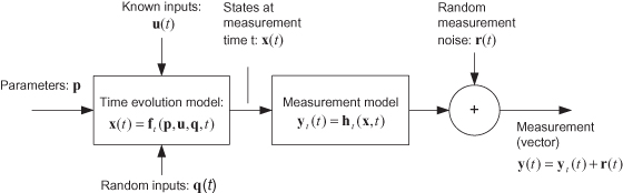
Noise-free measurements of the system output, y_t(t), are obtained from a linear or nonlinear transformation on the state x(t). Finally it is assumed that the actual measurements are corrupted by additive random noise r(t), although measurement noise is often not considered part of the forward model.

A polynomial in time is a simple example of a forward model. For example, the linear position of an object might be modeled as x(t) = p₁ + p₂t + p₃t² where t represents the time difference from a fixed epoch. A sensor may record the position of the object as a function of time and random noise may corrupt the measurements, that is, y(t) = x(t) + r(t). This is a one-dimensional example where neither process noise (q) nor forcing inputs (u) affect the measurements. The state will be multidimensional for most real-world problems.

The inputs p, u, q, and r may not exist in all models. If the random inputs represented by q(t) are present, the model is called stochastic; otherwise it is deterministic. In some cases q(t) may not be considered part of the forward model since it is unknown to us. Although the model of Figure 1.1 is shown to be a function of time, some models are time-invariant or are a function of one, two, or three spatial dimensions. These special cases will be discussed in later chapters. It is generally assumed in this book that the problem is time-dependent.

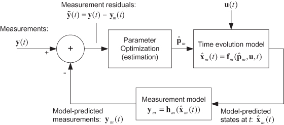
Figure 1.2 graphically shows the inverse modeling problem for a deterministic model. We are given the time series (or possibly a spatially distributed set) of “noisy” measurements y(t), known system inputs u(t), and models (time evolution and measurement) of the system. These models, f_m(p,u,t) and h_m(x), are unlikely to exactly match the true system behavior (represented by f_t(p,u,t) and h_t(x)), which are generally unknown to us. To perform the estimation, actual measurements y(t) are differenced with model-based predictions of the measurements y_m(t) to compute measurement residuals. The set of measurement residuals for the entire data span is processed by an optimization algorithm to compute a new set of parameter values that minimize some function of the measurement residuals. In least-squares estimation the “cost” or “loss” function to be minimized is the sum-of-squares, possibly weighted, of all residuals. Other optimization criteria will be discussed later. The new parameter values are passed to the time evolution and measurement models to compute another set of model-based predicted measurements. A new set of measurement residuals is computed for the entire data span and a new cost function is computed. If the models are linear, only one iteration is normally required to converge on parameters that minimize the cost function. If the models are nonlinear, multiple iterations will be required to compute the optimum.

The optimization process may update the estimates of p after each new measurement is received. This is called recursive estimation and is particularly useful when process noise q(t) is present in the system. This topic is discussed in Chapter 8 (Kalman filtering) and later chapters.

This inverse modeling summary was intended as a high-level description of estimation. It intentionally avoided mathematical rigor so that readers unfamiliar with estimation theory could understand the concepts before being swamped with mathematics. Those readers with significant estimation experience should not be discouraged: the math will quickly follow.

1.2 A BRIEF HISTORY OF ESTIMATION

Estimation theory started with the least-squares method, and earliest applications modeled motion of the moon, planets, and comets. Work by Johannes Kepler (1619) established the geometric laws governing motion of heavenly bodies, and Sir Isaac Newton (1687) demonstrated that universal gravitation caused these bodies to move in conic sections. However, determination of orbits using astronomical observations required long spans of data and results were not as accurate as desired—particularly for comets. In the mid-1700s it was recognized that measurement errors and hypothetical assumptions about orbits were partly responsible for the problem. Carl Friedrich Gauss claims to have first used the least-squares technique in 1795, when he was only 18, but he did not initially consider it very important. Gauss achieved wide recognition in 1801 when his predicted return of the asteroid Ceres proved to be much more accurate than the predictions of others. Several astronomers urged him to publish the methods employed in these calculations, but Gauss felt that more development was needed. Furthermore, he had “other occupations.” Although Gauss’s notes on the Ceres calculations appear contradictory, he probably employed an early version of the least-squares method. Adrien-Marie Legendre independently invented the method—also for modeling planetary motion—and published the first description of the technique in a book printed in 1806. Gauss continued to refine the method, and in 1809 published a book (Theoria Motus) on orbit determination that included a detailed description of least squares. He mentioned Legendre’s work, but also referred to his earlier work. A controversy between Gauss and Legendre ensued, but historians eventually found sufficient evidence to substantiate Gauss’s claim as the first inventor.

Gauss’s (1809) explanation of least squares showed great insight and may have been another reason that he is credited with the discovery. Gauss recognized that observation errors could significantly affect the solution, and he devised a method for determining the orbit to “satisfy all the observations in the most accurate manner possible.” This was accomplished “by a suitable combination of more observations than the number absolutely requisite for the determination of the unknown quantities.” He further recognized that “… the most probable system of values of the quantities … will be that in which the sum of the squares of the differences between the actually observed and computed values multiplied by numbers that measure the degree of precision is a minimum.”

Gauss’s work may have been influenced by the work of others, but he was the first to put all the pieces together to develop a practical method. He recognized the need for redundancy of observations to eliminate the influence of measurement errors, and also recognized that determining the most probable values implied minimizing observation residuals. He computed these measurement residuals using equations (models) of planetary motion and measurements that were based on an “approximate knowledge of the orbit.” This approach allowed iterative solution of nonlinear problems. Gauss reasoned that measurement errors would be independent of each other so that the joint probability density function of the measurement residuals would be equal to the product of individual density functions. Further he claimed that the normal density function would be

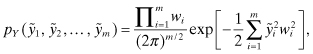
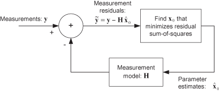
where w_i are weighting factors that take into account measurement errors. Gauss noted that the maximum of the probability density function is determined by maximizing the logarithm of the density function. For the assumed conditions, this is equivalent to minimizing the measurement residual sum-of-squares. Figure 1.3 shows the general structure of the least-squares method devised by Gauss, where vector y includes all measurements accumulated over a fixed period of time (if time is an independent variable of the problem).

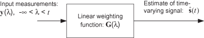
Improvements in the least-squares computational approach, statistical and probability foundations, and extensions to other applications were made by Pierre-Simon Laplace, Andrey Markov, and Friedrich Helmert after 1809. In the early 1900s Sir Ronald Fisher (1918, 1925) developed the maximum likelihood and analysis of variance methods for parameter estimation. However, no fundamental extensions of estimation theory were made until the 1940s. Until that time applications generally involved parameter estimation using deterministic models. Andrey Kolmogorov and Norbert Wiener were concerned with modeling unknown stochastic signals corrupted by additive measurement noise. The presence of random dynamic noise made the stochastic problem significantly different from least-squares parameter estimation. Kolmogorov (1941) analyzed transition probabilities for a Markov process, and the discrete-time linear least-squares smoothing and prediction problem for stationary random processes. Wiener (1949) independently examined a similar prediction problem for continuous systems. Wiener’s work was motivated by physical applications in a variety of fields, but the need to solve fire control and signal processing problems was a driving factor. This led him to study filtering and fixed-lag smoothing. Figure 1.4 shows a simplified version of the general problem addressed by Wiener filtering for multidimensional y(t) and s(t).

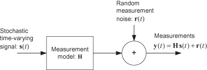
Message and measurement error processes are described by correlation functions or equivalently power spectral densities (PSD), and the minimum mean-squared error solution for the optimal weighting matrix G(t) is computed using the Wiener-Hopf integral equation in the time domain:

(1.2-1)

where R_sy(τ) = E[s(t)y^T(t − τ)], R_ss(τ) = E[s(t)s^T(t − τ)], E[·] denotes the expected value of random variables and it is assumed that either s(t), y(t), or both are zero mean. The correlation functions R_sy(τ) and R_ss(τ) are empirically obtained from sampled data, or computed analytically if the signal characteristics are known. The steady-state filter gain, G(t), is computed by factorization of the power spectral density function—a frequency domain approach. (Details of the method are presented later in Chapter 8.) The resulting filter can be implemented as either infinite impulse response (IIR)—where a recursive implementation gives the filter an “infinite” memory to all past inputs—or as finite impulse response (FIR) where the filter operates on a sliding window of data, and data outside the window have no effect on the output. Figure 1.5 shows the IIR implementation. Unfortunately the spectral factorization approach assumes an infinite data span, so the solution is not realizable. Wiener avoided this problem by assuming a finite delay in the filter, where the delay was chosen sufficiently long to make approximation errors small. Other extensions of Wiener’s work were made by Bode and Shannon (1950), and Zadeh and Ragazzini (1950). They both assumed that the dynamic system could be modeled as a shaping filter excited by white noise, which was a powerful modeling concept.

While Kolmogorov’s and Wiener’s works were a significant extension of estimation technology, there were few practical applications of the methods. The assumptions of stationary random processes and steady-state solutions limited the usefulness of the technique. Various people attempted to extend the theory to nonstationary random processes using time-domain methods. Interest in state-space descriptions, rather than covariance, changed the focus of research, and led to recursive least-squares designs that were closely related to the present Kalman filter. Motivated by satellite orbit determination problems, Peter Swerling (1959) developed a discrete-time filter that was essentially a Kalman filter for the special case of noise-free dynamics; that is, it still addressed deterministic rather than stochastic pro­blems. Events having the greatest impact on technology occurred in 1960 and 1961 when Rudolf Kalman published one paper on discrete filtering (1960), another on continuous filtering (1961), and a joint paper (Kalman and Bucy 1961) on continuous filtering. The papers used the state-space approach, computed the solution as minimum mean-squared error, discussed the duality between control and estimation, discussed observability and controllability issues, and presented the material in a form that was easy to understand and implement. The design allowed for nonstationary stochastic signals and resulted in a solution with time-varying gains. The Kalman filter was quickly recognized as a very important tool. Stanley Schmidt realized that Kalman’s approach could be extended to nonlinear problems. This led to its use for midcourse navigation on the National Aeronautics and Space Administration (NASA) Apollo moon program in 1961 (Schmidt 1981; McGee and Schmidt 1985).

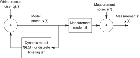
Figure 1.6 shows the generic model structure used as the basis of the Kalman filter design: q(t) and r(t) are white random noise and Φ(Δt) is the state transition matrix for the time interval Δt. Notice that the dynamic and measurement models are similar to those used in least-squares estimation, but they allow for the presence of random process noise, and the state vector x is defined using a moving epoch (t) rather than a fixed epoch (t₀).

More information on Gauss’s work and subsequent estimation history can be found in Gauss (1809), Bühler (1981), Sorenson (1970), Meditch (1973), Anderson and Moore (1979), Åström (1980), Tapley et al. (2004), Simon (2006), Grewal and Andrews (2001), Kailath (1968), Bennett (1993), and Schmidt (1981).

1.3 FILTERING, SMOOTHING, AND PREDICTION

The estimation problem is further classified as either filtering, smoothing, or prediction. Figure 1.7 graphically shows the differences. In the filtering problem the goal is to continuously provide the “best” estimate of the system state at the time of the last measurement, shown as t₂. When a new measurement becomes available, the filter processes the measurement and provides an improved estimate of the state at the new measurement time. In many systems—such as target tracking for collision avoidance or fire control—the goal is to provide an estimate of the state at some future time t₃. This is the prediction problem, and provided that the linear filter state estimate at t₂ is optimal, the predicted state is obtained by simply integrating the state vector at t₂:

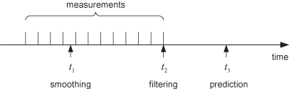
that is, the optimal linear predictor is the integral of the optimal linear filter. If the dynamic model is deterministic, the same approach can be applied to obtain the optimal state at any time prior to t₂. That is, integrate backward in time from t₂ to t₁. This assumption is implicit when using batch least-squares estimation: the epoch time at which the state is defined is arbitrary as the state at any other time may be obtained by analytic or numerical integration. However, when the dynamic model is subject to random perturbations—the stochastic case handled by Wiener or Kalman filtering—the optimal smoothed estimate at times in the past cannot be obtained by simple integration. As you may guess, the optimal smoothed estimate is obtained by weighting measurements near the desired smoothed time t₁ more than those far from t₁. Smoothed estimates must be computed using a time history of filter estimates, or information that is equivalent. Optimal smoothing is discussed in Chapter 9.

1.4 PREREQUISITES

Many early books on Kalman filtering included introductory chapters on linear and matrix algebra, state-space methods, probability, and random (stochastic) processes. This was desirable since few engineers at that time had good background in these areas. That situation has changed somewhat. We assume that the reader has been exposed to these topics, but may need a refresher course. Hence, the first appendix summarizes matrix algebra and the second summarizes probability and random process theory. Numerous references provide more background for those who want it. Particularly recommended are Papoulis and Pillai (2002), Kay (1988), Marple (1987), Cooper and McGillem (1967), Jazwinski (1970), Åström (1970), and Parzen (1960) for information on probability, stochastic processes, and spectral properties; DeRusso et al. (1965) for state-space methods and matrix operations; Lawson and Hanson (1974), Björck (1996), and Golub and Van Loan (1996) for least-squares estimation and matrix theory; and Kay (1988), Marple (1987), Gelb (1974), and Simon (2006) for material on several of these topics.

It is more important that the reader be familiar with matrix algebra than probability theory. Sufficient background is provided within the text to understand discussions involving stochastic processes, but it will be difficult to follow the material if the reader is not familiar with matrix algebra. Although somewhat less important, we also assume that the reader is familiar with Fourier, Laplace, and Z transforms. These topics are covered in many texts for various fields. Of the books previously mentioned, Cooper and McGillem (1967) and DeRusso et al. (1965) provide good background on transforms.

1.5 NOTATION

Unfortunately the notation used in estimation literature is not entirely consistent. This is partly due to the limited number of letters in the combined English and Greek alphabets, and the application of estimation to fields that each have their own notation. Even Kalman and Bucy used slightly different notations in different publications.

We tend to use Kalman’s and Bucy’s notation, but with modifications. Vectors are represented as bold lower case letters, and matrices are bold upper case letters. Dots above variables denote time derivative (), an overbar denotes the unconditional mean value of a random variable (), a “hat” denotes the mean value conditioned on knowledge of other random variables (), and a tilde denotes the error in a conditional mean ().

Variable x is generally used to denote the state vector. Unless otherwise stated, vectors are assumed to be column vectors. Functional dependence of one variable on another is expressed using parentheses [x(t)], discrete-time samples of a variable are denoted using subscripts [x_i = x(t_i)], and the state estimate at one time conditioned on measurement data (y) up to another time is denoted as . (Other authors sometimes use (–) to denote a priori estimates, , and (+) to denote a posteriori estimates, .)

Use of subscripts for time dependence may occasionally become confusing because subscripts are also used to denote elements of a vector or matrix. For example, A_jk usually denotes the (j,k) element of matrix A. If A is also a function of time t_i, one might use (A_i)_jk. Another alternative is to list the subscripts in parentheses, but this could also be ambiguous in that it implies functional dependence. We only show subscripts in parentheses when listing pseudo-code for algorithms. We also use the MATLAB/Fortran 90 “colon” notation to denote a range of a vector or array, that is, A(1 : n,i) denotes elements 1 to n of column i of matrix A, and A(:,i) denotes the entire column i. If rows or columns of A are treated as vectors in algorithms, a_:i denotes column i and a_i: denotes row i.

Even more confusing, we occasionally use subscripts separated by an underscore to denote a condition under which the variable is defined. The text should clarify the notation in these cases. Superscripts generally denote exponents of a variable, but there are a few exceptions. For example, s* is the complex conjugate of complex variable s. Exponents on matrices have the following meanings for matrix A: A^T is the transpose, A^H is the Hermitian (complex conjugate transpose), A⁻¹ is the inverse and A^# is the pseudo-inverse. These terms are defined in Appendix A.

Set notation is often used to define variables such as vectors and matrices. For example, A ∈ R^n×m is sometimes used to denote that A is a real-valued matrix having n rows and m columns, or x ∈ Rⁿ is a real vector with n elements. Another example is x(t), t ∈ [0,T) to indicate that variable x is defined over the time interval 0 ≤ t < T. Set notation is cumbersome for the purpose of this book, and potentially confusing. Hence we describe A as an n × m matrix, and x as an n-element vector.

Also, many probability texts use upper case variables to denote the domain of a random variable with lower case variables used to denote realizations of the variable, for example, . While mathematically more precise than , it is also cumbersome and usage is limited.

1.6 SUMMARY

We have shown how estimation can be viewed as an inverse modeling problem that accounts for the effects of measurement noise. Gauss and Legendre developed the least-squares method for deterministic models while Wiener and Kolmorgov developed a steady-state filtering approach for stationary stochastic models. Kalman, Bucy, and others extended the method to time-varying nonstationary stochastic systems using a state-space model. Table 1.1 compares various attributes of least-squares estimation and Kalman filtering. This table is partially a summary of Chapter 1, and partly an introduction to later chapters. Some terms have not yet been defined, but you can probably guess the meaning—details will be provided in later chapters. You may want to look at this table again after reading subsequent chapters.

TABLE 1.1: Comparison of Least-Squares Estimation and Kalman Filtering

Attribute	Least Squares (LS)	Kalman Filter (KF)
Batch versus recursive solution	Batch LS on finite data span (FIR). Recursive LS (IIR)	Recursive (IIR) on unlimited data span. Fixed interval smoother can provide “batch” solution on finite data span.
Real-time processing	Batch LS requires periodic execution. Recursive LS will eventually ignore new data unless re-initialized. Can also de-weight older data.	Ideal for real-time processing
Dynamic model	Deterministic	Stochastic: may be time-varying and nonstationary
Solution for nonlinear models	Iterative Gauss-Newton solution uses linear expansion at each iteration	Extended KF linearizes about current estimate at each measurement. Other approaches are available.
Inclusion of prior information	Yes: Bayesian solution No: Maximum likelihood or weighted least-squares solution	Standard KF requires prior estimate. Information KF can operate without prior.

The most important distinction between the least-squares and Kalman filtering methods is the allowance for process noise in the Kalman filter dynamic model; that is, the Kalman filter can handle stochastic problems while the least-squares method cannot. Other differences, such as batch versus recursive implementation, tend to be less important because either method can be made to perform similarly to the other.