
CHAPTER 5
LINEAR LEAST-SQUARES ESTIMATION: SOLUTION TECHNIQUES
This chapter discusses numerical methods for solving least-squares problems, sensitivity to numerical errors, and practical implementation issues. These topics necessarily involve discussions of matrix inversion methods (Gauss-Jordan elimination, Cholesky factorization), orthogonal transformations, and iterative refinement of solutions. The orthogonalization methods (Givens rotations, Householder transformations, and Gram-Schmidt orthogonalization) are used in the QR and Singular Value Decomposition (SVD) methods for computing least-squares solutions. The concepts of observability, numerical conditioning, and pseudo-inverses are also discussed. Examples demonstrate numerical accuracy and computational speed issues.
5.1 MATRIX NORMS, CONDITION NUMBER, OBSERVABILITY, AND THE PSEUDO-INVERSE
Prior to addressing least-squares solution methods, we review four matrix-vector properties that are useful when evaluating and comparing solutions.
5.1.1 Vector-Matrix Norms
The first is property of interest is the norm of a vector or matrix. Norms such as root-sum-squared, maximum value, and average absolute value are often used when discussing scalar variables. Similar concepts apply to vectors. The Hölder p-norms for vectors are defined as
(5.1-1)
The most important of these p-norms are
(5.1-2)
![]()
(5.1-3)
(5.1-4)
![]()
The l2-norm ![]() x
x![]() 2, also called the Euclidian or root-sum-squared norm, is generally the most often used. To apply these concepts to matrices, the elements of matrix A could be treated as a vector. For an l2-like norm, this leads to the Frobenius norm
2, also called the Euclidian or root-sum-squared norm, is generally the most often used. To apply these concepts to matrices, the elements of matrix A could be treated as a vector. For an l2-like norm, this leads to the Frobenius norm
(5.1-5)
One can also compute induced matrix norms based on the ability of matrix A to modify the magnitude of a vector, that is,
where the norms for A, Ax, and x need not be the same, but usually are. The l1-norm is
![]()
where a:j is the j-th column of A, and the l∞-norm is
![]()
where ai: is the i-th row of A. Unfortunately it is more difficult to compute an l2-norm based on this definition than a Frobenius norm. It turns out that ![]() A
A![]() 2 is equal to the square root of the maximum eigenvalue of ATA—or equivalently the largest singular value of A—but it is not always convenient to compute the eigen decomposition or SVD.
2 is equal to the square root of the maximum eigenvalue of ATA—or equivalently the largest singular value of A—but it is not always convenient to compute the eigen decomposition or SVD.
Two properties of matrix norms will be of use in the next sections. From definition (eq. 5.1-6) it follows that
and this can be extended to products of matrices:
However, the l2 and Frobenius matrix norms are unchanged by orthogonal transformations, that is,
(5.1-9)
![]()
More information on matrix-vector norms may be found in Dennis and Schnabel (1983), Björck (1996), Lawson and Hanson (1974), Golub and van Loan (1996), and Stewart (1998).
5.1.2 Matrix Pseudo-Inverse
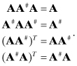
When matrix A is square and nonsingular, the equation Ax = b can be solved for x using matrix inversion (x = A−1b). When A is rectangular or singular, A does not have an inverse, but Penrose (1955) defined a pseudo-inverse A# uniquely determined by four properties:
(5.1-10)
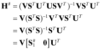
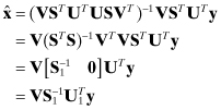
This Moore-Penrose pseudo-inverse is of interest in solving least-squares problems because the normal equation solution ![]() for y = Hx + r uses a pseudo-inverse; that is, H# = (HTH)−1HT is the pseudo-inverse of H. Notice that when H has more rows than columns (the normal overdetermined least-squares case), the pseudo-inverse (HTH)−1HT does not provide an exact solution—only the closest solution in a least-squares sense. This pseudo-inverse can be also written using the SVD of H
for y = Hx + r uses a pseudo-inverse; that is, H# = (HTH)−1HT is the pseudo-inverse of H. Notice that when H has more rows than columns (the normal overdetermined least-squares case), the pseudo-inverse (HTH)−1HT does not provide an exact solution—only the closest solution in a least-squares sense. This pseudo-inverse can be also written using the SVD of H
![]()
where U is an m × m orthogonal matrix, V is an n × n orthogonal matrix, and S = [S1 0]T is an m × n upper diagonal matrix of singular values (S1 is an n × n diagonal matrix). The pseudo-inverse is
(5.1-11)
where ![]() is the pseudo-inverse of S1. This equation shows that a pseudo-inverse can be computed even when HTH is singular (the underdetermined least-squares case). Singular values that are exactly zero are replaced with zeroes in the same locations when forming
is the pseudo-inverse of S1. This equation shows that a pseudo-inverse can be computed even when HTH is singular (the underdetermined least-squares case). Singular values that are exactly zero are replaced with zeroes in the same locations when forming ![]() . The term “pseudo-inverse” often implies an inverse computed for a rank deficient (rank < min(m,n)) H matrix rather than a full-rank inverse such as (HTH)−1HT. In this case the pseudo-inverse provides the minimal norm solution, as will be discussed in Section 5.8.
. The term “pseudo-inverse” often implies an inverse computed for a rank deficient (rank < min(m,n)) H matrix rather than a full-rank inverse such as (HTH)−1HT. In this case the pseudo-inverse provides the minimal norm solution, as will be discussed in Section 5.8.
5.1.3 Condition Number
Another useful matrix property describes the sensitivity of x in
to perturbations in A and b; that is, the magnitude of δx due to perturbations δA and δb in
(5.1-13)
![]()
Note that A can be a square matrix, but this is not a requirement. The following analysis of the problem is from Dennis and Schnabel (1983, p. 52), which is based on Wilkinson’s (1965) backward error analysis. First consider the effects of perturbation δb such that x + δx = A−1(b + δb) or
(5.1-14)
![]()
This equation applies for a square nonsingular A, but it also applies if A−1 is interpreted as a pseudo-inverse of a full-rank rectangular A. Using equation (5.1-7),
(5.1-15)
![]()
Equation (5.1-7) can also be used on equation (5.1-12) to obtain
(5.1-16)
![]()
Merging the two equations yields
(5.1-17)
![]()
Similarly for perturbation δA, (A + δA)(x + δx) = Ab, or ignoring the δAδx term,
(5.1-18)
![]()
Using (5.1-8),
(5.1-19)
![]()
or
(5.1-20)
![]()
In both cases the relative sensitivity is bounded by ![]() A
A![]()
![]() A
A![]() −1, which is called a condition number of A and is denoted as
−1, which is called a condition number of A and is denoted as
(5.1-21)
![]()
when using the corresponding lp induced matrix norm for A. Again these equations still apply if A−1 is replaced with A# when A is rectangular and full rank (rank = min(m,n)). Notice that κp(A) is unaffected by scaling of A that multiplies the entire matrix; that is, κp(αA) = κp(A). However, κp(A) is affected by scaling that affects only parts of A.
The effects of numerical errors (due to computational round-off) on minimal norm solutions for x in Ax = b are analyzed using κp(A). It can be shown that most numerical solution techniques limit ![]() δA
δA![]() /
/![]() A
A![]() to a constant (c) times the computer numerical precision (ε), so that
to a constant (c) times the computer numerical precision (ε), so that
![]()
Notice that κp(A) = 1 when A = αI, and κp(A) increases as A approaches singularity.
Example 5.1: Matrix Condition Number for Rank-2 Matrix
First consider
![]()
for which κ1(A) = α/α = 1. We use the l1-norm for convenience. This is an example of a well-conditioned matrix. Now consider
![]()
for which
![]()
Assuming that |β| < 1 (which is a condition for A to be nonsingular), ![]() A
A![]() 1 = 1, and
1 = 1, and ![]() A−1
A−1![]() 1 = 1/(1 − β2), so that
1 = 1/(1 − β2), so that
![]()
Hence as |β| → 1, κ1(A) → ∞. For example, if β = 0.999, κ1(A) = 500.25. It is obvious that solution of x in equation x = A−1b will become increasingly sensitive to errors in either A or b as |β| → 1.
As a third example, consider
![]()
for which κ1(A) = β if |β| > 1. A is clearly nonsingular, but can still have a large condition number when β is large. This demonstrates a problem in treating condition numbers as a measure of “closeness to singularity” or “non-uniqueness.” For κp(A) to be used as a test for observability (a term defined in the next section), matrix A should be scaled so that the diagonal elements are equal. The effects of scaling are often overlooked when condition numbers are used for tests of observability. This issue will be explored further in Section 5.7.
It is generally not convenient or accurate to compute condition numbers by inverting a matrix. Condition numbers can also be computed from the singular values of matrix A. Since A can be decomposed as A = USVT, where U and V are orthogonal, and A−1 = VS−1UT when A is square, then ![]() and
and ![]() where si are the singular values in S. Hence
where si are the singular values in S. Hence
(5.1-22)
However, it is computationally expensive to evaluate the SVD, so simpler methods are often used. One such method assumes that the A matrix has been transformed to an upper triangular form using an orthogonal transformation; that is, TTA = U where TTT = I and U is upper triangular. (This QR transformation is discussed in Section 5.3.) Since T is orthogonal, ![]() A2
A2![]() =
= ![]() U
U![]() 2 and
2 and ![]() A
A![]() F =
F = ![]() U
U![]() F. Bierman’s Estimation Subroutine Library (ESL) subroutine RINCON.F—used for examples in this chapter—computes the condition number
F. Bierman’s Estimation Subroutine Library (ESL) subroutine RINCON.F—used for examples in this chapter—computes the condition number
(5.1-23)
![]()
using the Frobenius norm because RINCON explicitly inverts U. κF(U) may be larger than κ2(U), although it is usually quite close.
Computation of κ2(U) without using the SVD depends upon computation of the matrix l2-norm, which is difficult to compute. Thus alternatives involving the l1-norm are often used. For the l1-norm of n × n matrix A,
(5.1-24)
![]()
In practice it is normally found that κ1(U) ≈ κ1(A), as will be shown in a later example. An estimate of κ1(U) can be computed using a method developed by Cline, Moler, Stewart, and Wilkinson (1979), and is included in the LINPACK linear algebra library (Dongarra et al. 1979). First, ![]() (where u:j is column j of U) is computed. Then a bound on
(where u:j is column j of U) is computed. Then a bound on ![]() U−1
U−1![]() 1 is computed from the inequality
1 is computed from the inequality
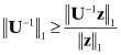
for any nonzero z. The appropriate z is chosen by solving UTz = e, where e is a vector of ±1’s with the signs chosen to maximize |zi| for i = 1, 2,…, n in sequence. Then Uy = z is solved for y (i.e., y = U−1U−Te), and the estimated κ1(U) is evaluated as
(5.1-25)
![]()
As noted by Dennis and Schnabel (1983, p.55) and Björck (1996, p. 116), even though ![]() y
y![]() 1/
1/![]() z
z![]() 1 is only a lower bound on
1 is only a lower bound on ![]() U−1
U−1![]() 1, it is usually close. Another κ1(U) estimator developed by Hagar and Higham is found in LAPACK (Anderson et al. 1999). This algorithm does not require transforming A to upper triangular form. It only requires computation of products Ax and ATx where x is a vector. Björck (1996, p. 117) claims that the estimates produced by this algorithm are sharper than those of the LINPACK algorithm.
1, it is usually close. Another κ1(U) estimator developed by Hagar and Higham is found in LAPACK (Anderson et al. 1999). This algorithm does not require transforming A to upper triangular form. It only requires computation of products Ax and ATx where x is a vector. Björck (1996, p. 117) claims that the estimates produced by this algorithm are sharper than those of the LINPACK algorithm.
5.1.4 Observability
Previous chapters have generally assumed that the system y = Hx + r is observable, but this term has not been clearly defined. Theoretical observability is defined in several ways that are equivalent:
1. The rank of the m × n matrix H must be n.
2. H must have n nonzero singular values.
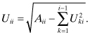
3. The rows of H must span the n-dimensional vector space such that any n-vector can be represented as
![]()
where hi: is row i of H.
4. The eigenvalues of HTH must be greater than zero.
5. The determinant of HTH must be greater than zero.
6. HTH must be positive definite; that is, xTHTHx > 0 for all nonzero x.
7. It must be possible to uniquely factor HTH as LLT (lower triangular) or UUT (upper triangular) where all diagonals of L or U are nonzero.
8.
![]() (where A = HTH) for i ≠ j is a necessary but not sufficient condition for observability.
(where A = HTH) for i ≠ j is a necessary but not sufficient condition for observability.
When the rank of H is less than n (or any of the equivalent conditions), the system is unobservable; that is, HTH of the normal equations is singular and a unique solution cannot be obtained. However, even when x is theoretically observable from a given set of measurements, numerical errors may cause tests for the conditions listed above to fail. Conversely, numerical errors may also allow tests for many of these conditions to pass even when the system is theoretically unobservable. Hence numerical observability may be different from theoretical observability. The matrix condition number is one metric used to determine numerical observability. Practical tests for observability are addressed in Section 5.7.
5.2 NORMAL EQUATION FORMATION AND SOLUTION
5.2.1 Computation of the Normal Equations
The normal equation for the weighted least-squares case of equation (4.2-3) is
(5.2-1)
![]()
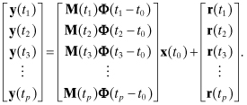
When the number of scalar measurements (m) in y is much larger than the number of unknowns (n) in x—which is usually the case—and explicit or implicit integration is required to compute H, it is generally most efficient to accumulate information in the normal equations individually for each measurement or set of measurements with a common time. That is, the measurement loop is the outer loop in forming b = HTR−1y and A = HTR−1H. For generality we assume that the state vector x is referenced to an epoch time t0, and that measurements y(ti) at other times ti for i = 1, 2, 3,…, p are modeled as the product of a measurement sensitivity matrix M(ti) and the state transition matrix from time t0 to ti; that is,
y(ti) may be a scalar or a vector, but the sum of the number of measurements for all p times is assumed to be m. If the independent variable in the model is not time but simply a measurement index, equation (5.2-2) still applies, but Φ(ti − t0) = I. In either case the total set of all measurements is represented as
(5.2-3)
The most commonly used software structure for solving the least-squares normal equation is:
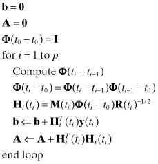
where R(ti)−1/2 is an inverse “square-root” factor of the measurement noise covariance matrix R(ti) at time ti; that is, R(ti) = R(ti)1/2R(ti)T/2 and R(ti)−1/2 = (R(ti)1/2)−1. The notation b ⇐ b + c means that b + c replaces b in memory. In most cases R(ti) is assumed to be a diagonal matrix with diagonal elements in row i equal to ![]() . Thus formation of M(ti)Φ(ti − t0)R(ti)−1/2 just involves dividing each row of M(ti)Φ(ti − t0) by σi(ti). If R(ti) is not diagonal, R(ti)1/2 is usually a lower triangular Cholesky factor of R(ti).
. Thus formation of M(ti)Φ(ti − t0)R(ti)−1/2 just involves dividing each row of M(ti)Φ(ti − t0) by σi(ti). If R(ti) is not diagonal, R(ti)1/2 is usually a lower triangular Cholesky factor of R(ti).
Notice that the total number of floating point operations (flops) required to accumulate the n × n matrix A and n-element vector b in equation (5.2-4) is mn(n + 3)/2 if only the upper triangular partition of A is formed (as recommended). It will be seen later that alternate algorithms require more than mn(n + 3)/2 flops. It will also be seen that the general structure of equation (5.2-4) can be applied even when using these alternate algorithms.
An example demonstrates how the special structure of certain partitioned problems can suggest alternate solution approaches.
Example 5.2: Partitioned Orbit Determination
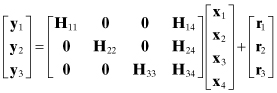
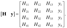
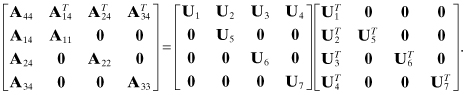
In some least-squares problems a subset of model states contribute to all measurements while other states influence only selected subsets of the measurements. For example, in orbit determination of a low-earth-orbiting satellite, ground station tracking biases only affect measurements from that ground station. For a case in which three ground stations track a satellite, the measurement sensitivity matrix H could have the structure
where
| y1 | includes all measurements from station #1 (for all passes), |
| y2 | includes all measurements from station #2, |
| y3 | includes all measurements from station #3, |
| x1, x2, x3 | are the measurement biases for ground stations 1, 2, and 3, respectively, |
| x4 | are the common states such as the satellite epoch orbit states and any other force model parameters, |
| Hij | is the measurement sensitivity matrix for measurement set i with respect to states j, |
| r1, r2, r3 | are the measurement noises for the three stations. |
Notice that this numbering scheme does not make any assumptions about measurement time order.
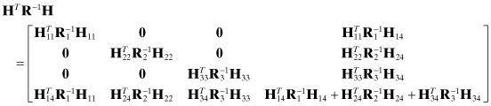
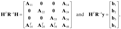
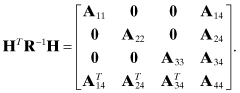
The information matrix for this problem is
and the information vector is
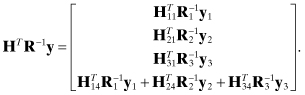
The zero partitions in HTR−1H allow the normal equation solution ![]() to be obtained in partitions without inverting the entire matrix. Specifically, for the case
to be obtained in partitions without inverting the entire matrix. Specifically, for the case
![]() can be solved for
can be solved for ![]() in partitions, starting with the common parameters. The partitioned solution is easily determined to be
in partitions, starting with the common parameters. The partitioned solution is easily determined to be
![]()
![]()
![]()
![]()
where
![]()
is the error covariance for ![]() . Likewise
. Likewise
![]()
![]()
![]()
are the error covariances for ![]() , respectively. Computation of the covariances between
, respectively. Computation of the covariances between ![]() , and
, and ![]() are left as an exercise for the reader. Hint: see the partitioned matrix solution in Appendix A.
are left as an exercise for the reader. Hint: see the partitioned matrix solution in Appendix A.
This example shows how it is possible to solve separately for subsets of states when some subsets only influence subsets of the measurements. This is a great advantage when the number of states and subsets is very large because it is only necessary to compute and store information arrays for the nonzero partitions. For example, when computing earth gravity field models, thousands of satellite arcs from multiple satellites are processed, and the orbit elements from each arc are solved for as separate states. This would not be practical without partitioning. For problems with a large number of states and ground stations (or equivalent “pass-dependent” parameters), the savings in computations and memory usage may be orders of magnitude.
Block partitioning of the measurement matrix also appears in other systems when the states are spatially distributed parameters and either the force model or measurement models have a limited spatial extent. Finite difference and finite element models of physical systems are another example of this structure.
Although the partitioned solution works best when using the normal equations, it is sometimes possible to exploit block partitioned structure when using some of the other least-squares solution techniques described below. An example appears in Section 5.3.
5.2.2 Cholesky Decomposition of the Normal Equations
In this section we address solution of the least-squares normal equations or equations that are equivalent to the normal equations. Consider the weighted least-squares normal equations of equation (4.2-3)
or for the Bayesian estimate,
Solution techniques for the two equations are identical because equation (5.2-6) can be viewed as equation (5.2-5) with the a priori estimate xa treated as a measurement. Hence we concentrate on equation (5.2-5). This can be solved by a number of methods. For example, Gauss-Jordan elimination can be used to transform (HTR−1H) to the identity matrix. This is done by computing both (HTR−1H)−1 and (HTR−1H)−1HTR−1y in one operation, or (HTR−1H)−1HTR−1y can be computed without inverting the matrix (Press et al. 2007, Section 2.1). It is important that pivoting be used in Gauss-Jordan elimination to maintain accuracy—particularly when HTR−1H is poorly conditioned. Another approach uses the LU decomposition to factor HTR−1H = LU where L is a lower triangular matrix and U is an upper triangular matrix. Then the L and U factors can be easily inverted to form P = (HTR−1H)−1 = U−1L−1. With partial pivoting, this has approximately the same accuracy as Gauss-Jordan elimination with full pivoting, but does not take advantage of the fact that HTR−1H is a positive definite symmetric matrix.
Cholesky decomposition of a positive definite symmetric matrix is similar to the LU decomposition but with the constraint that L = UT. That is,
(5.2-7)
![]()
Similar factorizations can also be defined using UUT where U is upper triangular, or as UDUT where U is unit upper triangular (1’s on the diagonal) and D is a diagonal matrix of positive values. The UDUT factorization has the advantage that square roots are not required in the computation. However, we work with UTU because that is the usual definition of Cholesky factors. The factorization can be understood using a three-state example.
Example 5.3: Cholesky Factorization
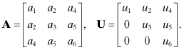
Consider the Cholesky factorization of a 3 × 3 positive definite symmetric matrix A = UTU:
(5.2-8)
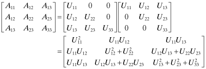
It is evident that the U elements can be computed starting from the upper left element:
(5.2-9)
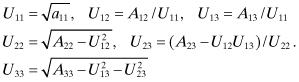
The general algorithm for a n × m matrix is
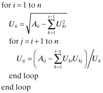
Note that the elements of U and the upper triangular portion of A can occupy the same storage locations because Aij is never referenced after setting Uij. The factorization can also be implemented in column order or as vector outer products rather than the row order indicated here (Björck 1996, Section 2.2.2).
The stability of the Cholesky factorization is due to the fact that the elements of U must be less than or equal to the diagonals of A. Note that
![]()
Hence numerical errors do not grow and the pivoting used with other matrix inversion methods is not necessary. However, Björck (1996, Section 2.7.4) shows that pivoting can be used to solve unobservable (singular) least-squares problems when HTR−1H is only positive semi-definite.
In coding Cholesky and other algorithms that work with symmetric or upper triangular matrices, it is customary to store these arrays as upper-triangular-by-column vectors such that
Use of vectors for array storage cuts the required memory approximately in half, which is beneficial when the dimension is large. For this nomenclature, the Cholesky algorithm becomes
(5.2-11)
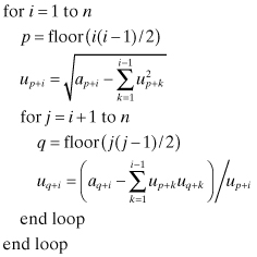
where floor(x) is the largest integer less than or equal to x. Again the elements of U and A can occupy the same storage locations.
To invert U, the equation UM = I is solved for M where M = U−1 is an upper triangular matrix; that is,
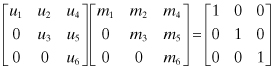
which leads to
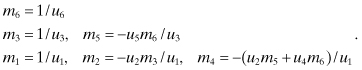
Again M and U may occupy the same storage. We leave it as an exercise for the reader to develop a general algorithm for computing M = U−1 and then forming A−1 = U−1U−T. This can also be implemented using the same storage as A. Hint: Subroutine SINV in software associated with this book and LAPACK routine DPOTF2 implement this algorithm, although the indexing can be somewhat confusing.
The number of flops required to Cholesky factor A = UTU is approximately n3/6, where a multiplication or division plus an addition or subtraction are counted as a single flop. n3/6 flops are also required to invert U, and the same to form A−1 = U−1U−T. Hence the total number of flops to invert A is about n3/2. This is half of the ∼n3 operations required to implement inversion based on LU decomposition or Gauss-Jordan elimination. However, since m is generally much greater than n, the flops required to invert HTR−1H are small compared with flops for computing HTR−1H and HTR−1y.
Use of the Cholesky factorization to invert HTR−1H has the potential advantage of greater accuracy compared with the LU or Gauss-Jordan elimination algorithms. However, the accuracy of the LU and Gauss-Jordan elimination can equal that of Cholesky factorization when full pivoting is used. Cholesky factorization is insensitive to scaling issues even without pivoting. That is, the states estimated using the least-squares method can be scaled arbitrarily with little effect on the numerical accuracy of the matrix inversion. This is demonstrated shortly in Example 5.4.
Example 5.4: Least Squares Using a Polynomial Model
Use of the polynomial model
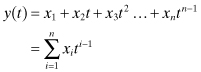
for least-squares data fitting results in a poorly conditioned solution when n values are not “small.” We evaluate the loss of accuracy for this polynomial model using 101 measurement samples separated in time by 0.01 s over the interval 0 to 1.0 s. For simplicity, the measurement noise variance is assumed to be 1.0, so R = I. The measurement matrix H for this case is
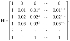
This structure, consisting of integer powers of variables, is called a Vandermonde matrix. Conditioning of Vandermonde matrices is very poor for even moderate values of n, and it is critical that calculations be performed in double precision. If possible, the problem should be restructured to use orthogonal basis functions such as Chebyshev polynomials. However, the polynomial problem offers a good test case for least-squares algorithms.
Notice that for the H matrix defined above,
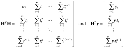
HTH and HTy for this particular problem can be efficiently calculated as shown using sums of powers of ti. However, we use the method described in Section 5.2.1.
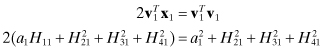
When evaluating accuracy of the solution, the quantity of most interest is the error in the estimated state:
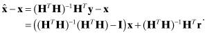
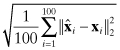
The first term should be zero and the second is the error due to measurement noise. The extent to which (HTH)−1(HTH) − I ≠ 0 is a measure of numerical errors in forming and inverting the normal equations. We use two metrics to evaluate accuracy of the polynomial solution. The first is the Frobenius norm,
where A = HTH. The second metric is the induced l1-norm
![]()
The base 10 logarithm of these metrics is computed as function of n when using double precision (53 bits mantissa) in IEEE T_floating format on a PC. We also tabulate expected precision, calculated as ![]() , computed during the Cholesky factorization of HTH.
, computed during the Cholesky factorization of HTH.
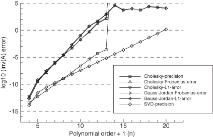
Figure 5.1 shows the results when using Cholesky factorization and Gauss-Jordan elimination with full pivoting to invert HTH. Figure 5.2 is a similar plot obtained when the first four columns of H are scaled by 100. Several conclusions can be drawn from these results:
1. Even with 101 measurements, no normal equation method will work for n > 13.
2. The Cholesky inversion is slightly more accurate than Gauss-Jordan elimination with full pivoting, but the difference is negligible. Gauss-Jordan elimination will continue to compute solutions for n > 13 even though all precision is lost.
3. The Cholesky precision calculation for number of digits lost,
tends to underestimate the actual loss of precision by a factor of about 10 for ηi < 8, and a factor of 104 as the matrix approaches singularity. In fact, the actual loss of precision seems to follow
although the reason for the factor of 1.3 is unknown. Nonetheless, ![]() is still a useful indicator of observability problems as it loosely tracks the loss of precision. Any solution where
is still a useful indicator of observability problems as it loosely tracks the loss of precision. Any solution where ![]() is greater than eight should be highly suspect.
is greater than eight should be highly suspect.
4. The “SVD precision” line in the figures is the expected precision, calculated as log10[1.1 × 10⁻¹⁶ × κ2(H)] from the singular values of H. Since formation of HTH doubles the condition number, the expected precision of the normal equations is log10(1.1 × 10⁻¹⁶) + 2 log10(κ2(H)), which has twice the slope of the “SVD precision” line. This roughly matches the actual “Cholesky” or “Gauss-Jordan” inversion accuracy up to the point where they lose all precision. Hence the precision predicted from the condition number of H is appropriate for the normal equation solution.
5. Scaling of the first four columns of the H matrix by 100 degrades the accuracy of the matrix inversion by the same factor. However, it has negligible effect on calculation of ![]() . This result is somewhat misleading because multiplying the columns of H by 100 implies that the corresponding elements of x must be divided by 100 if y is unchanged. Hence the fact that the errors increased by 100 in Figure 5.2 implies that the Cholesky factorization is relatively insensitive to scale changes.
. This result is somewhat misleading because multiplying the columns of H by 100 implies that the corresponding elements of x must be divided by 100 if y is unchanged. Hence the fact that the errors increased by 100 in Figure 5.2 implies that the Cholesky factorization is relatively insensitive to scale changes.
FIGURE 5.1: Least-squares normal equations inversion accuracy using polynomial model.
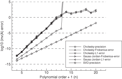
FIGURE 5.2: Least-squares normal equations inversion accuracy using polynomial model with H(:,1:4) multiplied by 100.
Monte Carlo evaluation is also used as an alternate check on numeric accuracy. One hundred independent samples of state vector x were randomly generated where each individual element of x was obtained from a Gaussian random number generator using a standard deviation of 1.0. Then y = Hx (with no measurement noise) was used to calculate ![]() . The two metrics used for the evaluation are averaged values of the l2- and l∞-norms:
. The two metrics used for the evaluation are averaged values of the l2- and l∞-norms:
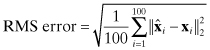
and
![]()
where ![]() is the maximum absolute value of the elements in
is the maximum absolute value of the elements in ![]() over all samples of
over all samples of ![]() . Figures 5.3–5.4 show the results plotted on a log scale. The root-mean-squared (RMS) error is approximately equal to the Frobenius norm of A−1A − I in Figures 5.1 and 5.2 for the same conditions, and the maximum error is approximately equal to the l1-norm of A−1A − I. This suggests that numerical errors in (HTH)−1(HTH) are positively correlated rather than independent. Also notice that the RMS errors in
. Figures 5.3–5.4 show the results plotted on a log scale. The root-mean-squared (RMS) error is approximately equal to the Frobenius norm of A−1A − I in Figures 5.1 and 5.2 for the same conditions, and the maximum error is approximately equal to the l1-norm of A−1A − I. This suggests that numerical errors in (HTH)−1(HTH) are positively correlated rather than independent. Also notice that the RMS errors in ![]() are about 20 to 4000 times larger than
are about 20 to 4000 times larger than ![]() (labeled “Cholesky precision”). Again when columns of H are scaled by 100, the errors are about 100 times larger than when unscaled.
(labeled “Cholesky precision”). Again when columns of H are scaled by 100, the errors are about 100 times larger than when unscaled.
FIGURE 5.3: Monte Carlo evaluation of LS normal equations solution accuracy using polynomial model.
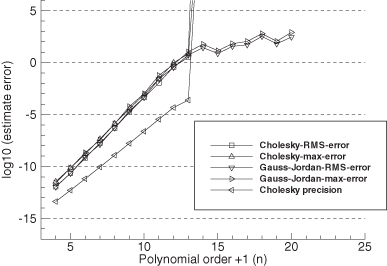
FIGURE 5.4: Monte Carlo evaluation of LS normal equations solution accuracy using polynomial model with H(:,1:4) multiplied by 100.
Another advantage of the Cholesky factorization is that it automatically provides information about numerical conditioning of HTR−1H. Notice the second line in equation (5.2-10):
When ![]() is very close in magnitude to Aii, the subtraction will result in a loss of precision. This happens when HTR−1H is nearly singular. The metric
is very close in magnitude to Aii, the subtraction will result in a loss of precision. This happens when HTR−1H is nearly singular. The metric
indicates the number of numerical digits lost when processing column i. The maximum ηi for i = 1 to n is somewhat correlated with log10(“condition number”) for matrix HTR−1H. Hence when the number of digits lost approaches half of the total floating point precision digits, the accuracy of the solution should be suspect. The following example demonstrates these concepts.
5.3 ORTHOGONAL TRANSFORMATIONS AND THE QR METHOD
As noted previously, solution of the normal equations is not the only method that can be used to compute least-squares estimates. Previous sections used the normal equations because they are easily understood and often used in practice. However, the normal equations are more sensitive to the effects of numerical round-off errors than alternative algorithms. This can be understood by expanding the information matrix using the SVD of matrix L−1H where R = LLT:
Notice that equation (5.3-1) is an eigen decomposition of HTR−1H since V is an orthogonal matrix and STS is the diagonal matrix of eigenvalues. Hence the condition number for HTR−1H is twice as large as that for L−1H since the singular values are squared in STS. Thus a least-squares solution technique that does not form HTR−1H would be expected to have approximately twice the accuracy of a solution that inverts (directly or indirectly) HTR−1H.
One solution method that avoids formation of the normal equations is based on the properties of orthogonal transformations. To use this QR method (originally developed by Francis [1961] for eigen decomposition), it is necessary that the measurement equation be expressed as y = Hx + r where E[rrT] = I. If E[rrT] = R ≠ I, first factor R as R = LLT and then multiply the measurement equation by L−1 as
![]()
so that E[L−1rrTL−T] = I. In most cases R is diagonal so this normalization step just involves dividing the rows of y and H by the measurement standard deviation for each measurement. Then the QR algorithm proceeds using L−1y as the measurement vector and L−1H as the measurement matrix. For simplicity in notation, we assume that the normalization has been applied before using the QR algorithm, and we drop the use of L−1 in the equations to follow. It should be noted that when measurement weighting results in a “stiff system” (one in which certain linear combinations of states are weighted much more heavily than others), additional pivoting operations are necessary in the QR algorithm to prevent possible numerical problems (Björck 1996, Section 2.7.3). Other approaches for including the weights directly in the QR algorithm are also possible (Björck 1996, p. 164). This topic is addressed again in Chapter 7 when discussing constraints.
In the QR algorithm the m × n measurement matrix H is factored as H = QTR, or equivalently QH = R, where Q is an m × n orthogonal matrix and R is an upper triangular m × n matrix. Although Q and R are commonly used as the array symbols in the QR algorithm (for obvious reasons), this notation will be confusing in this book because we have already used Q for the discrete state noise covariance matrix and R for the measurement noise covariance. Hence we substitute array T for Q and U for R in the QR algorithm so that H is factored as H = TTU. (The U matrix represents an upper triangular matrix, not the orthogonal matrix of the SVD algorithm.) This implies that the measurement equation is multiplied by T = (TT)−1 (since T is orthogonal) such that TH = U; that is,
(5.3-2)
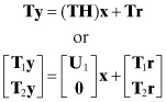
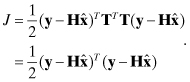
where ![]() , T1 is n × m, T2 is (m − n) × m, and U1 is n × n. The least-squares cost function is unchanged by this transformation because
, T1 is n × m, T2 is (m − n) × m, and U1 is n × n. The least-squares cost function is unchanged by this transformation because
(5.3-3)
This can also be written as
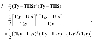
Since the second term in equation (5.3-4) is not a function of ![]() , the value of
, the value of ![]() that minimizes J is
that minimizes J is
where T1y is an n-vector. If H is of rank n, the upper triangular n × n matrix ![]() is easily computed by back-solving
is easily computed by back-solving ![]() . Notice that the cost function is J = (T2y)T(T2y)/2 for the
. Notice that the cost function is J = (T2y)T(T2y)/2 for the ![]() of equation (5.3-5).
of equation (5.3-5).
The error covariance matrix for ![]() is
is
(5.3-6)
![]()
Since T is orthogonal, it does not amplify numerical errors, and the condition number of U1 is the same as that of H. Furthermore, U1 is never squared in the solution, so the condition number does not increase as it does when forming the normal equations. Hence sensitivity to numerical errors is approximately one-half that of the normal equations.
The T matrix is computed using elementary Givens rotations, orthogonal Householder transformations, or Modified Gram-Schmidt (MGS) orthogonalization (see Lawson and Hanson 1974; Bierman 1977b; Dennis and Schnabel 1983; Björck 1996; Press et al. 2007). It will be seen in the next section that it is not necessary to explicitly calculate T.
5.3.1 Givens Rotations
Givens rotations are defined as
![]()
where c2 + s2 = 1. The coefficients can be interpreted as cosine and sine functions of an angle, but trigonometric functions are not required. A Givens rotation can be applied to zero an element of a vector. For example
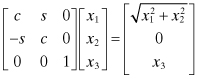
when ![]() and
and ![]() . Individual Givens rotations can be sequentially applied to zero all elements in a column of the H matrix below the diagonal where only the diagonal element is modified at each step. Then this sequence of operations is applied for remaining columns until TH = U where T represents the product of all individual rotations. Since the individual rotations do not modify the magnitude of the H columns, the transformation is numerically stable. Givens rotations are typically used to modify a few elements of a matrix or vector. While Givens rotations can be used to triangularize matrices, Householder transformations require one-half or fewer flops compared with “fast” versions of Givens rotations (Björck 1996, p. 56; Golub and Van Loan 1996, p. 218). However, Givens rotations offer more flexibility in zeroing specific sections within a matrix, and can be less sensitive to scaling problems (Björck 1996).
. Individual Givens rotations can be sequentially applied to zero all elements in a column of the H matrix below the diagonal where only the diagonal element is modified at each step. Then this sequence of operations is applied for remaining columns until TH = U where T represents the product of all individual rotations. Since the individual rotations do not modify the magnitude of the H columns, the transformation is numerically stable. Givens rotations are typically used to modify a few elements of a matrix or vector. While Givens rotations can be used to triangularize matrices, Householder transformations require one-half or fewer flops compared with “fast” versions of Givens rotations (Björck 1996, p. 56; Golub and Van Loan 1996, p. 218). However, Givens rotations offer more flexibility in zeroing specific sections within a matrix, and can be less sensitive to scaling problems (Björck 1996).
5.3.2 Householder Transformations
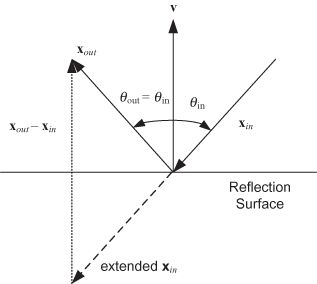
Householder transformations are called reflection operations because they behave like specular reflection of a light ray from a mirror (Fig. 5.5)
FIGURE 5.5: Specular reflection.
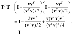
An elementary Householder reflection is defined as
(5.3-7)
![]()
where v is the vector normal to the hyperplane of reflection. It is easily shown that T is orthogonal:
The reflection property can be seen by differencing the output and input vectors,
(5.3-8)
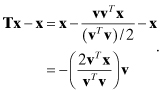
The sign of all components of x in direction v are reversed by the transformation. A sequence of Householder transformations can be used to zero the lower triangle of the measurement H matrix as shown in the example below.
Example 5.5: Use of Householder Transformations to Triangularize an Overdetermined System of Equations
Assume that four measurements are used to solve for three states where the measurement equation is y = Hx + r. We wish to multiply the left- and right-hand side of that equation by an orthogonal transformation T that makes TH an upper triangular matrix. We start by appending the measurement vector y to H to form an augmented measurement matrix:
The first transformation should eliminate H21, H31, and H41. Since the Householder transformation produces output vector
![]()
(where x1 is defined as the first column of H), it is apparent that the last three elements of v1 should equal the last three elements of x1, with ![]() . Let v1 = [a1 H21 H31 H41]T with a1 to be defined such that
. Let v1 = [a1 H21 H31 H41]T with a1 to be defined such that
or
![]()
Thus
![]()
To minimize numerical cancellation, it is better to use the same sign (above) as the sign of H11; that is,
![]()
Thus the transformed first column of H equals
![]()
Notice that this transformation preserves the magnitude of the vector, which is a desirable property for numerical stability. The remaining columns of [H y] are also modified by the transformation using
![]()
where xj is sequentially defined as each remaining column of [H y]. Then the process is repeated to zero the two (modified) elements of the second column below the diagonal using
![]()
Finally the modified H43 is zeroed using
![]()
Notice that each subsequent transformation works with one fewer elements in vj than the preceding transformation (vj−1) since it only operates on H columns from the diagonal down. The three transformations (corresponding to the three columns) are applied as
![]()
to produce the upper triangular matrix U and transformed vector Ty. In implementing this algorithm it is only necessary to store the current vi vector at step i, not the transformation matrix T.
The total number of flops required to triangularize the m × (n + 1) matrix [H y] is approximately n2(m − n/3), which is about twice the flops required to form the normal equation. Hence there is a penalty in using the QR algorithm, but the benefit is greater accuracy.
Example 5.6: Upper Triangular Factors of Sparse Normal Equations
In Example 5.2, the information matrix from the normal equations was assumed to have the structure
If one attempts to find an upper triangular matrix U such that UUT = HTR−1H, it is found that U will generally not contain zero partitions. However, if the state ordering is changed so that common parameters represented by x4 are moved to the top of the state vector, then the structure is changed to
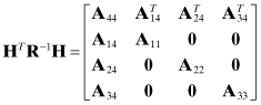
which can be factored as
Hence it is possible to develop a version of the QR algorithm that only operates with the nonzero partitions of U when processing measurements from a given ground station; for example, one need not include U6 and U7 when processing measurements from ground station #1 (corresponding to U5 on the diagonal). However, U1, U2, U3, U4 must be included when processing all measurements that are affected by the common parameters. The unused matrix partitions may be swapped in and out from disk to memory as needed. Implementation of this block partitioning using the QR method is more difficult than for the normal equations, but the savings can still be substantial.
5.3.3 Modified Gram-Schmidt (MGS) Orthogonalization
Another approach that can be used to triangularize a matrix is the Modified Gram-Schmidt (MGS) orthogonalization. In this method, the columns of H are sequentially transformed to a set of orthogonal columns. In the original Gram-Schmidt algorithm, the columns could gradually lose orthogonality due to numerical errors, with consequent loss of accuracy. The modification used in MGS first normalizes the columns at each step, with the result that the numerical errors are bounded. A row-oriented version of MGS for computing the QR decomposition
![]()
where H is m × n, U is n × n, y is m × 1, and z is n × 1 is implemented as follows:

Notice that T is not explicitly formed, but the wk vectors (k = 1 : n) contain the information required to generate T. Björck (1996, p. 65) shows that the MGS QR method applied to least-squares problems is equivalent to the Householder QR method for a slightly modified problem. Rather than use the Householder QR method to directly triangularize the [H y] matrix, it is applied to an augmented matrix with n rows of zeroes added at the top:
![]()
This corresponds to the modified measurement equation
![]()
Then a sequence of Householder transformations, denoted as T, is applied to obtain:
(5.3-9)
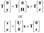
where T is an orthogonal (n + m) × (n + m) matrix,
![]()
and U = TH is an upper triangular n × n matrix. A recursive version of this algorithm (where the upper rows may already contain U and z arrays) is presented in Chapter 7 when discussing recursive least squares.
The least squares cost function is not modified by these changes, as shown by
(5.3-10)
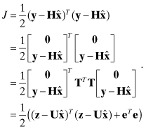
Provided that the upper triangular n × n matrix U is of rank n, ![]() minimizes J with the result that J = eTe/2.
minimizes J with the result that J = eTe/2.
Throughout this book we use “Householder QR” to mean the standard Householder QR method, “MGS QR” to mean the MGS/augmented Householder method (since they are equivalent), and “QR” algorithm to refer to either.
Golub and Van Loan (1996, p. 241) note that the MGS QR method has the same theoretical accuracy bounds as Householder QR, provided that it is implemented as an augmented system so that transformations also operate on y (as described above). However, several investigators have found that the MGS QR method is slightly more accurate than alternative orthogonalization methods (Björck 1996, p. 66), although the reason is not clear. Björck notes that the Householder QR method is sensitive to row permutations of H, whereas MGS is almost insensitive because it zeroes entire columns of H rather than just from the diagonal down. Björck suggests that when using the Householder QR method for weighted least-squares problems, the rows should be sorted in decreasing row norm before factorization, or column pivoting should be used. Unfortunately sorting in decreasing row norm order does not always solve the problem, as will be shown later.
Another benefit of the MGS QR approach is that measurements need not be processed all at once in a single batch, which is desirable (to avoid storing H) when n and m are large. That is, measurements may be processed in small batches (e.g., 100) where the nonzero U and z arrays from one batch are retained when processing the next batch. However, to implement this approach, additional terms must be included in the “row-oriented version of MGS” algorithm listed above. This recursive procedure is, in fact, the measurement update portion of Bierman’s (1977b) Square Root Information Filter (SRIF) that will be discussed in Chapter 10. Recursive updating of the Householder QR method can also be accomplished using Givens rank-1 updates (Björck 1996, p. 132). For more information on orthogonal transformations and the QR algorithm see Lawson and Hanson (1974), Björck (1996), Dennis and Schnabel (1983), Golub and Van Loan (1996), Bierman (1977b), and Press et al. (2007).
5.3.4 QR Numerical Accuracy
To evaluate the numerical accuracy of the QR algorithm, we again examine the error in the state estimate due to numerical errors only. Using equation (5.3-5),
However, ![]() is likely to underestimate the actual errors since it ignores errors in forming U1. Therefore, Monte Carlo evaluation of
is likely to underestimate the actual errors since it ignores errors in forming U1. Therefore, Monte Carlo evaluation of ![]() , where y = Hx, is deemed a more reliable indicator of numerical errors. Numerical results using the QR algorithm for our example polynomial problem are given later in Section 5.6.
, where y = Hx, is deemed a more reliable indicator of numerical errors. Numerical results using the QR algorithm for our example polynomial problem are given later in Section 5.6.
5.4 LEAST-SQUARES SOLUTION USING THE SVD
Another technique based on orthogonal transformations, the SVD, can also be used to solve the least-squares problem. As before, we start by computing the SVD of the measurement matrix: H = USVT where U is an m × m orthogonal (not upper triangular) matrix, V is an n × n orthogonal matrix, and S is an m × n upper diagonal matrix. When m > n (the overdetermined case), the SVD can be written as
![]()
where U1 is n × n, U2 is (m − n) × n, and S1 is n × n. U2 is the nullspace of H as it multiplies 0. Hence it is not needed to construct a least-squares solution and is often not computed by SVD algorithms. Golub and Van Loan (1996, p. 72) call SVD solutions without the U2 term a “thin SVD.”
The least-squares solution can be obtained by substituting this replacement for H in the cost function and then setting the gradient to zero. However, it is easier to make the substitution in the normal equations ![]() to obtain:
to obtain:
(5.4-1)
where ![]() is the n × n diagonal matrix of inverse singular values and
is the n × n diagonal matrix of inverse singular values and ![]() is the transpose of the first n columns of U. The error in the least-squares estimate is
is the transpose of the first n columns of U. The error in the least-squares estimate is
![]()
Hence either the magnitude of elements in ![]() or the Monte Carlo statistics on
or the Monte Carlo statistics on ![]() can be used as a measure of numerical accuracy. Numerical results for our polynomial problem are given in Section 5.6.
can be used as a measure of numerical accuracy. Numerical results for our polynomial problem are given in Section 5.6.
The most successful SVD algorithms use Householder transformations to first convert H to a bi-diagonal form (nonzero elements are limited to the diagonal, and either immediately above or below the diagonal). Then iterative or divide-and-conquer techniques are used to converge on the singular values in S. Many methods are based on a routine written by Forsythe et al. (1977, chapter 9), which was based on the work of Golub and Reinsch (see Wilkinson and Reinsch 1971; Dongarra et al. 1979; Stoer and Bulirsch 1980). Since the solution is iterative, the total number of flops varies with the problem. It can be generally expected that the computational time required to obtain an SVD solution will be five or more times greater than the time required to solve the problem using the QR methods, although the ratio will be problem-dependent.
One popular reference (Press et al. 2007) states that the SVD is the method of choice for solving most least-squares problems. That advice may reflect the experience of the authors, but one suspects that their experience is limited to small problems. The arguments for using the SVD are
1. The SVD is numerically accurate and reliable.
2. The SVD automatically indicates when the system of equations is numerically unobservable, and it provides a mechanism to obtain a minimal norm solution in these cases.
3. The SVD provides information on linear combinations of states that are unobservable or weakly observable.
However, the first two arguments are not by themselves convincing (because QR methods also have these properties), and there are several reasons why use of the SVD should be avoided for problems where the number of measurement is large and much greater than the number of unknowns:
1. Multistep algorithms used to compute the SVD may result in an accumulation of numerical errors, and they can potentially be less accurate than the QR algorithm.
2.
In some real problems tens of thousands of measurements are required to obtain an accurate solution with thousands of unknown states. Hence storage of the H matrix may require gigabytes of memory, and computational time for the SVD may be an order of magnitude (or more) greater than for the QR algorithms. If observability is to be analyzed via the SVD, the QR algorithms should first be used to transform the measurement equations to the compact n-element form z = Ux + e. Then the SVD can be used on z and U with no loss of accuracy. This is the method recommended by Lawson and Hanson (1974, p. 290) when mn is large and m ![]() n. Results later in this chapter show that accuracy is enhanced and execution time is greatly reduced when using this procedure.
n. Results later in this chapter show that accuracy is enhanced and execution time is greatly reduced when using this procedure.
3. Most other solution techniques also provide information on conditioning of the solution. Minimal norm solutions in unobservable cases can be computed using other techniques.
4. Use of the SVD to obtain a minimal-norm solution in cases where the system of equations is unobservable implicitly applies a linear constraint on the estimated parameters. That is, the state estimate from the pseudo-inverse is a linear combination of the model states. If the only use of the least-squares model is to obtain smoothed or predicted values of the same quantities that are measured, this is usually acceptable. However, in many problems the states represent physical parameters, and estimation of those states is the goal. Other estimation applications attempt to predict quantities not directly measured, or predict to untested conditions. In these cases it is often not acceptable to compute a minimal-norm (pseudo-inverse) solution when the measurements alone are not sufficient to obtain a solution—this is demonstrated in a later example. Better approaches either obtain more measurements or use prior information.
5.5 ITERATIVE TECHNIQUES
Linear least-squares problems can also be solved using iterative techniques that generally fall into two categories: linear iteration and Krylov space. Iterative methods for solving nonlinear least-squares problems are discussed in Chapter 7. Before addressing iterative approaches, we first review sparse matrix storage methods because iterative methods are mostly used for large sparse systems.
5.5.1 Sparse Array Storage
One commonly used sparse array storage method places all nonzero elements of sparse m × n matrix A in a real vector a of dimension p. The column index of elements in a are stored in integer vector ja, and another integer vector ia of dimension m + 1 stores the ja and a indices of the first element belonging to each A row. That is, elements in row i of matrix A will be found in elements ia(i) to ia(i + 1) − 1 of vectors ja and a, where ja(k) specifies the column index for a(k). Hence a matrix-vector product c = Ab can be implemented using this storage scheme as follows:
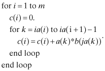
The transpose product c = ATb is implemented in a slightly different order:
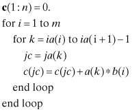
where we have used the MATLAB/Fortran 90 convention for specifying partitions of arrays and vectors; that is, c(1 : n) = c(i), 1 ≤ i ≤ n. Although both of the above matrix-vector multiplications involve some “hopping” in computer memory, compilers effectively optimize the above loops and execution can be efficient. Other sparse storage methods are possible (Björck 1996, p. 270; Anderson et al. 1999; Press et al. 2007, p. 71), and they may be more efficient for operations involving specific types of sparse arrays. Finally it should be noted that matrix-matrix products can be efficient even when sparsity is evaluated “on-the-fly.” For example, a general-purpose version of C = AB, where A is sparse, can be implemented without using sparse storage methods as follows:
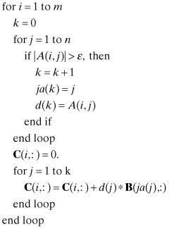
where ε is a threshold for nonzero elements (e.g., 10−60 or even 0). Temporary n-element vectors d and ja are used to store the nonzero element values and column indices of each A row. This method becomes somewhat less efficient when B is a vector, but even when A is a full matrix the execution time may only increase slightly compared with a normal matrix product.
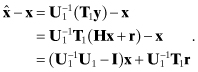
5.5.2 Linear Iteration
Iterative techniques can be used to refine an approximate solution of the equation Ax = b. The simplest method is linear iteration. Let ![]() be the exact solution to the normal equations (
be the exact solution to the normal equations (![]() ) and let
) and let ![]() be an approximate solution. Then assuming linearity,
be an approximate solution. Then assuming linearity,
(5.5-1)
![]()
which can be arranged to obtain
The quantity on the right should be evaluated before inverting HTH to obtain ![]() . Iterative refinement of this type is rarely used because accuracy is usually not much better than that of direct normal equation solutions. This statement also applies when HTH is Cholesky factored and the factors are back-solved to compute the solution to equation (5.5-2). The loss of precision in forming HTH is the limiting factor.
. Iterative refinement of this type is rarely used because accuracy is usually not much better than that of direct normal equation solutions. This statement also applies when HTH is Cholesky factored and the factors are back-solved to compute the solution to equation (5.5-2). The loss of precision in forming HTH is the limiting factor.
Other classical iteration techniques include Jacobi, Gauss-Seidel, successive overrelaxation (SOR), and Richardson’s first-order method (Kelley 1995; Björck 1996). These methods split the A matrix in Ax = b as A = A1 + A2 where A1 is a nonsingular matrix constructed so that A1x = (b − A2x) can be easily solved for x.
5.5.3 Least-Squares Solution for Large Sparse Problems Using Krylov Space Methods
Another category of iterative techniques is used to solve large sparse linear least-squares problems when it is not practical to store the entire information matrix HTH in computer memory. HTH generally fills in sparsity present in the original H matrix, and thus the storage requirements can be prohibitive. However, several Krylov space methods can solve the least-squares problem using H without forming HTH.
A Krylov subspace is defined as κk(A,x) = span{x,Ax,A2x,…,Ak−1x} where A is an n × n matrix and x is an n-element vector. Krylov space methods are iterative techniques used to either find the zeros of an affine function Ax − b = 0, or to locate the minimum of a multidimensional cost function J = (y − Hx)T(y − Hx). Krylov space algorithms fall into three classes. The first, conjugate gradient (CG) methods, assume that A is square and positive definite symmetric (Kelley 1995, Section 2.4; Björck 1996, Section 7.4). CG solvers work well with sparse array storage and are often used to solve finite-difference and finite-element problems. Unlike steepest descent methods for minimization problems, they do not take negative gradient steps. Rather, they attempt to take a sequence of steps that are orthogonal to previous steps within the Krylov subspace and in directions that minimize the cost function. As a worst case, CG algorithms should converge exactly when the number of iterations equals the number of unknown states, but if the conditioning is poor, this may not happen because of numerical errors. Furthermore, the convergence rate is unacceptably slow when the number of unknowns is thousands or hundreds of thousands. Conversely, CG algorithms can converge in tens of iterations if the conditioning is good. The bi-CG stabilized (Bi-CGSTAB) algorithm is one of the most successful of the CG methods applicable to general square matrices (see Van der Vorst 1992; Barrett et al. 1993, p.27; Kelley 1995, p. 50). Bi-CGSTAB can also handle square positive definite nonsymmetric A matrices, but convergence may be slower than for symmetric A.
The second class of Krylov space algorithms also takes a sequence of steps that are orthogonal to previous steps, but rather than recursively accumulating information “summarizing” past search directions—as done in CG solvers—these methods store past basis vectors. Because of this, storage requirements increase as iterations proceed. Implementations usually limit the storage to a fixed number of past vectors. Generalized minimum residual (GMRES) and ORTHOMIN are two of the most successful algorithms in this class (see Vinsome 1976; Kelley 1995; Barrett et al. 1993). ORTHOMIN and GMRES also work directly with overdetermined (nonsquare) H matrices to minimize a quadratic cost function.
This author found that the Bi-CGSTAB method converged faster than ORTHOMIN or GMRES when solving steady-state groundwater flow problems of the form Ax − b = 0. However, Bi-CGSTAB requires that matrix A be square, so it can only be used for least-squares problems when starting with the normal equations. This is undesirable because the condition number of HTH is twice that of H, and convergence of CG solvers is a function of the conditioning. Also the sparsity of HTH is generally much less than that of H, so storage and computations may greatly increase.
The third class of Krylov space methods was designed to work directly with least-squares problems. The most popular methods include CG on the normal equations to minimize the residual (CGNR; Barrett et al. 1993, p. 18; Kelley 1995, p. 25; Björck 1996, p. 288) and LSQR (Paige and Saunders 1982). CGNR is also called CGLS by Paige and Saunders. Even though these methods do not form HTH, they are still affected by the doubling of the condition number implied by forming HTH. CGNR and LSQR both use the measurement equations ![]() and HTv = 0, and iterate many times until the residuals are acceptably small. The LSQR algorithm attempts to minimize the effect of conditioning problems by solving the linearized least-squares problem using a Lanczos bi-diagonalization approach. LSQR is claimed to be more numerically stable than CGNR. Storage and computations are generally low, but for many flow-type problems, the performance of the LSQR algorithm without preconditioning appears to be almost identical to that of CG solutions on the normal equations. That is, the iterations tend to stall (do not reduce the residual error) after a few thousand iterations, and they can produce a solution that is unacceptable (Gibbs 1998).
and HTv = 0, and iterate many times until the residuals are acceptably small. The LSQR algorithm attempts to minimize the effect of conditioning problems by solving the linearized least-squares problem using a Lanczos bi-diagonalization approach. LSQR is claimed to be more numerically stable than CGNR. Storage and computations are generally low, but for many flow-type problems, the performance of the LSQR algorithm without preconditioning appears to be almost identical to that of CG solutions on the normal equations. That is, the iterations tend to stall (do not reduce the residual error) after a few thousand iterations, and they can produce a solution that is unacceptable (Gibbs 1998).
The convergence rate of Krylov space methods can be greatly improved if preconditioning is used to transform H or HTH to a matrix in which the eigenvalues are clustered close to 1. This can be implemented as either left or right preconditioning; for example, the root-finding problem Hx = y can be preconditioned as
(5.5-3)
![]()
where SL and SR are the left and right preconditioning matrices. Left preconditioning modifies scaling of the measurement residuals—which may be desirable in poorly scaled problems—while right preconditioning modifies scaling of the state x. Generally either left or right preconditioning is used, but not both. For the least-squares problem, direct preconditioning of HTH is not desirable because this destroys matrix symmetry. Rather, preconditioning is of the form
(5.5-4)
![]()
The goal is to find matrix SL or SR such that ![]() is close to the identity matrix. Preconditioning can either be applied as a first step where SLHSR is explicitly computed, or the multiplication can be included as part of the CG algorithm. Commonly used preconditioners include scaling by the inverse diagonals of HTH (the sum-of-squares of the columns of H), incomplete sparse Cholesky decomposition of the form LLT + E = HTH where E is small, incomplete LU decomposition for square H, or polynomial preconditioning (see Simon 1988; Barrett et al. 1993; Kelley 1995; Björck 1996). Diagonal scaling is generally not very effective and it can sometimes be difficult to compute incomplete Cholesky factors or polynomial preconditioners.
is close to the identity matrix. Preconditioning can either be applied as a first step where SLHSR is explicitly computed, or the multiplication can be included as part of the CG algorithm. Commonly used preconditioners include scaling by the inverse diagonals of HTH (the sum-of-squares of the columns of H), incomplete sparse Cholesky decomposition of the form LLT + E = HTH where E is small, incomplete LU decomposition for square H, or polynomial preconditioning (see Simon 1988; Barrett et al. 1993; Kelley 1995; Björck 1996). Diagonal scaling is generally not very effective and it can sometimes be difficult to compute incomplete Cholesky factors or polynomial preconditioners.
Another alternative to direct application of the CGNR method changes variables and inverts ![]() in partitions, where the partitions of H are implicitly inverted using other methods. This approach is somewhat similar to the red-black partitioning (Dongarra et al. 1991; Barrett et al. 1993, section 5.3) often used in iterative solution of sparse systems, and it can also be interpreted as a form of preconditioning. Numerical conditioning for the CG solver is improved because the dimension of the system to be solved is reduced. For flow and similar models resulting from finite-difference equations, those portions of the H matrix can be (implicitly) inverted efficiently using nonsymmetric preconditioned CG (PCG) solvers such as the Bi-CGSTAB method.
in partitions, where the partitions of H are implicitly inverted using other methods. This approach is somewhat similar to the red-black partitioning (Dongarra et al. 1991; Barrett et al. 1993, section 5.3) often used in iterative solution of sparse systems, and it can also be interpreted as a form of preconditioning. Numerical conditioning for the CG solver is improved because the dimension of the system to be solved is reduced. For flow and similar models resulting from finite-difference equations, those portions of the H matrix can be (implicitly) inverted efficiently using nonsymmetric preconditioned CG (PCG) solvers such as the Bi-CGSTAB method.
The CGNR algorithm applied to equation ![]() is given below. Initial values of the residual and scaled state are computed as
is given below. Initial values of the residual and scaled state are computed as
(5.5-5)
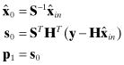
where S is a right preconditioning matrix. Then the CGNR iterations for i = 1, 2, … are
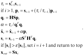
The LSQR algorithm (Paige and Saunders 1982) without preconditioning is initialized as
(5.5-7)

The LSQR iterations for i = 1, 2,… are
(5.5-8)
where ![]() is the residual vector norm
is the residual vector norm ![]() . Iterations stop if any of these tests are satisfied:
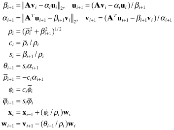
. Iterations stop if any of these tests are satisfied:
(5.5-9)
ATOL, BTOL, and CONLIM are user-specified tolerances and cond(A) is an estimate of the condition number of A as explained by Paige and Saunders (1982). To obtain a solution accurate to six digits, suggested values for ATOL and BTOL are 10−6, and the suggested CONLIM is ![]() where RELPR is the relative precision of the computer (e.g., 1.1 × 10⁻¹⁶ for double precision in IEEE T_floating). Preconditioning can be applied to LSQR or CGNR by redefining the A matrix.
where RELPR is the relative precision of the computer (e.g., 1.1 × 10⁻¹⁶ for double precision in IEEE T_floating). Preconditioning can be applied to LSQR or CGNR by redefining the A matrix.
The primary function of an iterative least-squares solver is to obtain a solution faster and with less storage than a direct method such as QR. If the estimate error covariance matrix or log likelihood function is required, one final iteration of a direct method must be used.
Example 5.7: Groundwater Flow Modeling Calibration Problem
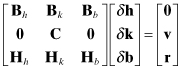
Consider a flow modeling least-squares problem (Porter et al. 1997) consisting of three linearized matrix equations:
where
| δh | are perturbations in hydraulic “head” at each node (n total) of a three-dimensional (3-D) finite difference grid, |
| δk | are perturbations in hydraulic conductivity at each node of a 3-D finite difference grid, |
| δb | are perturbations in p flow common parameters such as boundary conditions, |
| Bh = ∂f/∂h and Bk = ∂f/∂k | are n × n linearizations of the steady-state flow equation f(h,k,b) = 0 where f is the net flow to the nodes, |
| Bb = ∂f/∂b | is a n × p linearization of the steady-state flow equation f(h,k,b) = 0, |
| C | is a “soft” n × n spatial continuity conductivity constraint implemented as a 3-D autoregressive model, |
| v | is the conductivity constraint error at each node, |
| Hh | is the m × n measurement partial matrix (Jacobian) for hydraulic head measurements (each measurement is a function of head at four surrounding nodes), |
| Hk | is the m × n measurement partial matrix for hydraulic conductivity measurements (each measurement is a function of conductivity at four surrounding nodes), |
| Hb | is the m × p measurement partial matrix for hydraulic conductivity measurements with respect to common parameters (usually Hb = 0), and |
| r | is random measurement noise. |
All the above arrays are very sparse because each node connects to six (or less) other nodes. Typically only a few hundred head and conductivity measurements are available for site models consisting of 104 to 106 nodes. Hence the spatial continuity “pseudo-measurement” conductivity constraint is required to obtain a solution.
Since the first (flow) equation is a hard constraint and the square Bh matrix should be nonsingular, ![]() can be substituted to obtain the reduced equations
can be substituted to obtain the reduced equations
![]()
Since square matrix C is formed using an autoregressive model applied to nearest neighbors, it should also be nonsingular. This suggests that C can be used as a right preconditioner to obtain the modified measurement equation
![]()
Notice that the CGNR operations in equation (5.5-6) involving H appear as either (HS)pi or (HS)Tqi—a matrix times a vector. Hence ![]() can be evaluated as follows:
can be evaluated as follows:
1. z = C−1pi is computed using the Bi-CGSTAB solver (use incomplete LU decomposition preconditioning with the same fill as the original matrix, and red-black partitioning),
2. ![]() is computed using the Bi-CGSTAB solver (again use incomplete LU decomposition preconditioning with the same fill as the original matrix, and red-black partitioning),
is computed using the Bi-CGSTAB solver (again use incomplete LU decomposition preconditioning with the same fill as the original matrix, and red-black partitioning),
3. a = Hkz − Hhs.
Likewise ![]() can be evaluated using a similar sequence of operations. The substitution procedure can also be used for terms involving the boundary condition parameters.
can be evaluated using a similar sequence of operations. The substitution procedure can also be used for terms involving the boundary condition parameters.
When using this procedure for the groundwater flow modeling calibration problem, CGNR convergence is usually achieved in less than 100 CGNR iterations even when using 200000 node models (Gibbs 1998). Although this problem is unusual in that the number of actual measurements (not pseudo-measurements) is much smaller than the number of unknowns, the solution techniques can be applied to other 2-D or 3-D problems.
Example 5.8: Polynomial Problem Using CGNR and LSQR Solvers
The CGNR solver was also tested on the polynomial problem of Example 5.4. Right diagonal preconditioning was based on the inverse l2-norms of the columns of H, so the columns of HS were normalized to one. However, the results did not change significantly without preconditioning. Table 5.1 lists the results for CGNR and LSQR when using ε = 10−13 for CGNR and ATOL = BTOL = 10−6 for LSQR. For n < 8, the CGNR solver achieved accuracy comparable to Cholesky solutions of the normal equations, and the LSQR accuracy was almost as accurate as the QR algorithm for n < 9. This is not an entirely fair comparison because coding of the LSQR algorithm (LSQR 1982) was far more sophisticated than the elementary algorithm used for CGNR. For n ≥ 9, both the CGNR and LSQR solutions were unacceptable. (In interpreting the values of Table 5.1, recall that the x samples were generated with a standard deviation of 1.0) These results are compared with the other solution methods in the next section.
TABLE 5.1: CGNR and LSQR Accuracy on Least-Squares Polynomial Problem
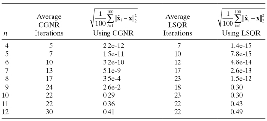
Both algorithms may perform better when using alternate preconditioners. We again caution that results for simple problems should not be interpreted as general characteristics applicable to all large-scale problems.
5.6 COMPARISON OF METHODS
We now compare numerical results when using different least-squares methods on the polynomial problem of Example 5.4 and on another problem. Execution times are also discussed.
5.6.1 Solution Accuracy for Polynomial Problem
The following examples discuss solution accuracy for the basic polynomial model of Example 5.4 and minor variations.
Example 5.9: Polynomial Problem
Figure 5.6 shows the 100-sample Monte Carlo RMS solution errors
for six different least-squares solution techniques versus polynomial order. As before, results are plotted on a log scale. Also shown are the accuracies obtained using condition numbers computed as the maximum ratio of singular values, and as κF(U) = ![]() U
U![]() F
F![]() U−1
U−1![]() F, which uses the Frobenius norm of the upper triangular U matrix produced by the QR method and its inverse (as discussed in Section 5.1.3). The plotted variables are labeled as follows:
F, which uses the Frobenius norm of the upper triangular U matrix produced by the QR method and its inverse (as discussed in Section 5.1.3). The plotted variables are labeled as follows:
1. Cholesky-RMS-error: the RMS error obtained when using the normal equations solved using Cholesky factorization.
2. Gauss-Jordan-RMS-error: the RMS error obtained when using the normal equations solved using Gauss-Jordan elimination.
3. QR-RMS-error: the RMS error obtained when using the QR method. Unless stated otherwise, the QR method is implemented using the MGS algorithm.
4. SVD-RMS-error: the RMS error obtained when using SVD. Unless stated otherwise, the SVD results are computed using the LAPACK DGESDD divide-and-conquer routine.
5. CGNR-RMS-error: the RMS error obtained when using CGNR method.
6. LSQR-RMS-error: the RMS error obtained when using LSQR method.
7. QR precision#: the accuracy computed as 1.1e-16 × condition number κF(U) = ![]() U
U![]() F
F![]() U−1
U−1![]() F.
F.
8. SVD precision: the accuracy computed as ![]()
FIGURE 5.6: Monte Carlo evaluation of LS solution accuracy using polynomial model.

The conclusions from Figure 5.6 are:
1. Errors of the normal equation method solved using Cholesky factorization and Gauss-Jordan method are approximately equal in magnitude up to the point at which all precision is lost (n = 13). These errors grow at twice the rate at which the condition numbers κ2(H) or κF(U) grow with polynomial order.
2. The condition number estimates κ2(H) and κF(U) closely agree for this problem. Although not shown in the plot, the LINPACK condition number estimate κ1(U) ≈ κ1(A) closely follows the other two estimates.
3. Errors of the SVD solution closely follow the accuracy computed using the condition numbers κ2(H) and κF(U). When using the LAPACK DGESVD (SVD using QR iteration) subroutine, the errors are similar to those of DGESDD, but those of the numerical recipes (Press et al. 2007) SVDCMP routine are approximately 5.5 (= log10 0.74) times larger.
4. Errors of the MGS QR method are a factor of approximately 3.5 (= log10 0.54) smaller than those of the LAPACK SVD methods. When the QR method is changed to use the Householder QR method, the errors are a factor of 12.6 (= log10 1.10) greater, or about 3.6 times greater than those of the LAPACK SVD methods.
5. When the MGS QR method is first used to transform [H y] to [U z], and then either the LAPACK or Numerical Recipes SVD routine is used on [U z], the estimation errors are comparable to those of the direct MGS QR method; that is, 3.5 times smaller than when the SVD is used directly on H. This is unexpected because the SVD methods first transform H to a nearly upper triangular matrix using Householder transformations.
6. Errors of the CGNR method at first closely follow those of the Cholesky and Gauss-Jordan methods up to n = 7, but then deteriorate rapidly. No indication of algorithm failure (such as reaching the maximum number of iterations) was given.
7. Errors of the LSQR method at first closely follow those of the SVD method, but LSQR then loses all precision at n = 9. LSQR produced a “termination flag” indicating that “The system A*X = B is probably not compatible. A least-squares solution has been obtained which is sufficiently accurate, given the value of ATOL.” However, the flag did not indicate complete failure.
Based on comments by Björck regarding the sensitivity of the QR method to row-norm ordering, the row order of H was changed from smallest norm to largest (as in Example 5.4), to largest to smallest. Figure 5.7 shows the result: errors of the normal equation and SVD methods increased very slightly, but the changes are barely noticeable in the plot. The lack of sensitivity to row ordering was also observed when the Householder QR method replaced the MGS QR method. (This result is counter to Björck’s suggestion that sorting by decreasing row norm will minimize numerical errors.) However, errors when using the Householder QR method are more than an order of magnitude greater than those obtained using the MGS QR method, as shown in Figure 5.8.
FIGURE 5.7: Monte Carlo evaluation of LS solution accuracy using polynomial model with H rows reordered by decreasing norm.
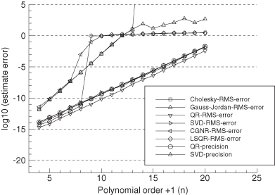
FIGURE 5.8: Monte Carlo evaluation of LS solution accuracy using QR methods on polynomial model with H rows reordered by decreasing norm.
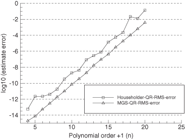
Example 5.10: Polynomial Problem with H(:,1:4) Multiplied by 100
As before, we examine the effects of scaling the first four columns of H by 100. Figure 5.9 shows the result. Compared with Figure 5.6, all the curves for n > 4 increase by a factor of 100 (= log10 2.0), except that the LSQR method breaks down for n ≥ 7 rather than 9. However, this example is not entirely realistic because standard deviations of the first four states in the Monte Carlo simulation are the same (1.0) as the remaining states, so these four states contribute 100 times more to the measurements than the other states. In Figure 5.10 the standard deviations of the first four states are set to 0.01, so all states contribute equally to the measurements. Notice that compared with Figure 5.9, the RMS errors drop by a factor of about 100 and are again comparable to those of Figure 5.6.
FIGURE 5.9: Monte Carlo evaluation of LS solution accuracy using polynomial models: H(:,1:4) multiplied by 100.
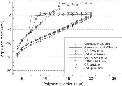
FIGURE 5.10: Monte Carlo evaluation of LS solution accuracy using polynomial models: H(:,1:4) multiplied by 100 and x(1:4) scaled by 0.01.
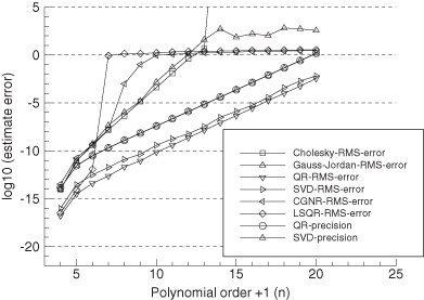
Notice, however, that QR and SVD condition numbers are still 100 times larger in Figure 5.10 than in Figure 5.6 since they are computed from H and are not dependent on actual measurements y or the states x. Recall that the condition number is defined as a relative error sensitivity, so this behavior is expected. This emphasizes a deficiency of using condition numbers to evaluate the importance of individual states to the solution, or of using condition numbers to infer observability. While condition numbers are useful in evaluating sensitivity of the solution to numerical errors and are not affected by scaling the entire H matrix, they are affected by relative scaling of measurements and states. This topic is discussed again in Section 5.7.
Finally, we note that the loss of numerical accuracy demonstrated above for the polynomial model can be entirely avoided by using basis functions that are orthogonal (or nearly orthogonal) over the fit interval 0 ≤ t ≤ 1. Figure 5.11 shows the 100-sample RMS estimate error, maximum error, and Cholesky precision versus model order when using a Chebyshev polynomial model and the normal equations solved with Cholesky factorization. Notice that the estimate errors are always less than 10−14 regardless of model order. The measurement residual magnitudes are also less than 10−14 over the fit interval, and they remain less than 10−14 for predictions over the next second (1 ≤ t ≤ 2). This accuracy is remarkable considering the results obtained using ordinary polynomials. Use of an orthogonal polynomial results in a least-squares information matrix (HTR−1H) that is diagonal, and therefore inversion is very accurate. Use of other basis functions that are orthogonal over the fit interval, such as Fourier series, should also have comparable accuracy.
FIGURE 5.11: Monte Carlo evaluation of LS solution accuracy using Chebyshev polynomial models.
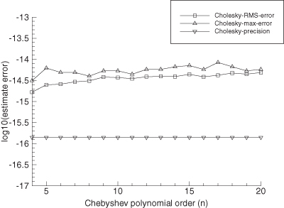
Example 5.11: Quasi “Bi-Diagonal” H
While the polynomial example is a good test case for evaluating the effects of poor conditioning, it may not be representative of many real-world problems. For example, results on the polynomial problem indicate that normal equation methods quickly lose all accuracy and should be avoided. However, normal equation methods (particularly Cholesky factorization) are used successfully on most least-squares problems. Therefore, an alternate evaluation test case similar to some real-world problems (but still simple) should be instructive. As before, we use a model with 101 (= m) measurements and 4 to 20 (= n) states. However, each row of the H matrix has three nonzero elements: two approximately on the diagonal and the third in the last column. For example, when m = 8 and n = 6, H has the structure
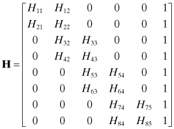
where the first two elements in each row i are linear interpolations from the diagonal, computed as
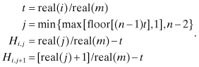
The floor function is the largest integer smaller than or equal to the real argument, and real converts an integer variable to floating point. Hence each measurement can be viewed as a linear interpolation on a local “position,” plus a common bias parameter. Using m = 101, the numerical results for the least-squares solution methods are shown in Figure 5.12. We notice the following:
1. The largest condition number for n = 40 is about 1160. Compared with the polynomial problem, this is a very well-conditioned case.
2. All methods except CGNR produce results accurate to more than 12.5 digits. The CGNR solution method is much less accurate than the others.
3. The LSQR solution is the most accurate of all up to n = 22, but then breaks down.
4. The accuracy of all other solution methods is similar, with the MGS QR solution somewhat better, and the SVD solution at times the worst. Interestingly, the normal equation Cholesky method is more accurate than the SVD for all n > 8.
5. The QR and SVD condition number accuracy bounds are again close, and roughly characterize the estimate errors. However, the SVD estimate errors are almost always larger than the condition number accuracy bound, and the QR estimate errors are almost always smaller.
FIGURE 5.12: Monte Carlo evaluation of LS solution accuracy using “bi-diagonal” H.
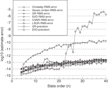
These results show that the relative solution accuracy can be problem-dependent, but the MGS QR method can usually be relied upon as accurate. Even the Cholesky normal equation method works very well for well-conditioned problems. The major problem in using normal equation methods is in recognizing when conditioning is a problem. When using Cholesky factorization, the loss-of-precision metric ![]() from equation (5.2-12) should always be monitored, and a more accurate algorithm should be used when
from equation (5.2-12) should always be monitored, and a more accurate algorithm should be used when ![]() is greater than half of the machine computational precision digits; for example, 8 digits lost when precision is 16 digits.
is greater than half of the machine computational precision digits; for example, 8 digits lost when precision is 16 digits.
5.6.2 Algorithm Timing
Execution time is also an important criteria when evaluating least-squares solution methods because least-squares methods are sometimes used on problems with thousands (occasionally tens of thousands) of states. Table 5.2 lists the approximate flop count and execution times for solution methods used on the polynomial problem with n = 13. This polynomial order is large enough so that n3 ![]() n2 and the n2 terms can be ignored. It is also the order at which the normal equation methods have lost accuracy, but this is irrelevant when computing execution times. In all cases the algorithms were executed 100,000 times so that timing was not significantly affected by clock precision. All LAPACK Basic Linear Algebra Subprograms (BLAS) were compiled with default optimization rather than using special object code optimized for the PC. Although the execution times in Table 5.2 may seem negligibly small, execution times tend to grow as either n3 or mn2. Since the state size of least-squares problems continues to grow with the capabilities of available computers, it is not unusual to have execution times measured in hours or even days. Hence algorithm execution time can be important.
n2 and the n2 terms can be ignored. It is also the order at which the normal equation methods have lost accuracy, but this is irrelevant when computing execution times. In all cases the algorithms were executed 100,000 times so that timing was not significantly affected by clock precision. All LAPACK Basic Linear Algebra Subprograms (BLAS) were compiled with default optimization rather than using special object code optimized for the PC. Although the execution times in Table 5.2 may seem negligibly small, execution times tend to grow as either n3 or mn2. Since the state size of least-squares problems continues to grow with the capabilities of available computers, it is not unusual to have execution times measured in hours or even days. Hence algorithm execution time can be important.
TABLE 5.2: FLOPS and Timing of Least-Squares Solution Methods: Polynomial (n = 13)
| Method | Approximate Flops | Time (Microsec)a |
| Normal equations with Cholesky inversion | mn2/2 + n3/2 | 41 |
| Normal equations with Gauss-Jordan inversion | mn2/2 + n3 | 61 |
| Householder QR | mn2 − n3/3 | 75 (79 for LAPACK) |
| MGS QR | mn2 | 50 |
| MGS QR plus SVD on R (numerical recipes SVDCMP)b | mn2 + (14/3 + 6k)n3 | 58 |
| SVD on H computing full V and n columns of U (numerical recipes SVDCMP)b | (6 + 4k)mn2 + (2k − 1)n3 | 285 |
| SVD on H computing full U, V (LAPACK divide and conquer DGESDD)c | unknown | 830 |
| SVD on H computing full V and n columns of U (LAPACK divide and conquer DGESDD)c | unknown | 368 |
| SVD on H computing full V and n columns of U (LAPACK bi-diagonal QR iteration DGESVD)c | unknown | 362 |
| SVD on H computing full V and no U (LAPACK bi-diagonal QR iteration DGESVD)c | unknown | 273 |
aAll code used double precision, compiled with default optimization (O4) and executed on 3.0 GHz P4 PC.
bk in the flop count is the variable number of internal iterations.
cLAPACK compiled with generic BLAS using default (O4) optimization.
Flop counts indicate that the MGS QR method should take twice the execution time as the normal equations with Cholesky factorization, but in practice it only takes 22% more time for this problem and is 33% faster than the Householder QR method. MGS QR is also generally the most accurate algorithm. Note that the MGS QR method followed by the SVD only takes 16% more time than the MGS QR method alone, while direct use of the thin SVD requires at least 724% as much time. Computation of the full U matrix in the SVD requires much more time and is of little benefit for general least-squares solutions. The relative performance of LAPACK may be better when used for large problems with a machine-specific BLAS.
Table 5.3 shows the algorithm timing for the “bidiagonal H” case when m = 2000 and n = 200. In this case the Householder QR algorithm is the fastest with MGS QR only slightly slower. It is surprising that both QR methods are much faster than the normal equations with Cholesky factorization. QR methods are generally slower than normal equations with Cholesky factorization, but not by a factor of two as would be expected from the flop count. Also notice that the “full U” SVD methods (computing all of U) are at least 5.4 times slower than the MGS QR method.
TABLE 5.3: FLOPS and Timing of Least-Square Solution Methods: “Bi-Diagonal” H, n = 200, m = 2000
| Method | Time (millisecond)a |
| Normal equations with Cholesky inversion | 378 |
| Normal equations with Gauss-Jordan inversion | 472 |
| Householder QR | 120 |
| MGS QR | 126 |
| MGS QR plus SVD on R (numerical recipes SVDCMP) | 126 + 249 = 375 |
| SVD on H computing full V and n columns of U (numerical recipes SVDCMP) | 2234 |
| SVD on H computing full U, V (LAPACK divide and conquer DGESDD)b | 5258 |
| SVD on H computing full V and n columns of U (LAPACK divide and conquer DGESDD)b | 683 |
| SVD on H computing full V and n columns of U (LAPACK bi-diagonal QR iteration DGESVD)b | 858 |
| SVD on H computing full V and no U (LAPACK bi-diagonal QR iteration DGESVD)b | 336 |
aAll codes used double precision, compiled with default optimization (O4) and executed on 3.0 GHz P4 PC.
bLAPACK compiled with generic BLAS using default (O4) optimization.
Relative execution times of the algorithms may be quite different when used on large-scale problems or on different computers, but these results suggest trends in expected performance.
5.7 SOLUTION UNIQUENESS, OBSERVABILITY, AND CONDITION NUMBER
Theoretical observability of states x in measurement equation y = Hx + r was defined in Section 5.1.4 by various conditions directly or indirectly implying that all singular values of H must be greater than zero. In Section 5.1.3 the matrix condition number κp(H) was defined as a “scale-free” measure of the relative sensitivity of x to relative numerical errors in H or y. These two concepts are related but not necessarily equivalent. Example 5.4 demonstrated that both the condition number and relative errors in the least-squares solution ![]() are affected by scaling of the H columns, but when the elements of x are also adjusted so that the magnitude of y is unchanged, then the errors in
are affected by scaling of the H columns, but when the elements of x are also adjusted so that the magnitude of y is unchanged, then the errors in ![]() return to the unscaled values.
return to the unscaled values.
Condition numbers κp(H), or more specifically the relative magnitudes of the smallest to the largest singular values, are often used to determine whether specific states or linear combinations of states are observable. The fundamental problem in this approach is that singular values are properties of H, and they do not take into account the relative magnitudes of states, measurements and measurement noise.
Consider a reordered version of the two-state measurement model y = Hx + r used in Example 5.1:
![]()
The singular values of H are β and 1, so κ2(H) = β. If β = 1018 and operations are conducted in 16-digit precision, the wide range in singular values suggests that the second state is unobservable and should be eliminated from the system. However, the system is fully observable, so the ratio of singular values is not a sufficient measure of observability. Now consider three possibilities:
1.
|x1| ≅ 1 and |x2| ≅ 1, but β is large so y1 is extremely sensitive (possibly because of different units) to x1. Hence if E(rrT) = I, the weighted least-squares estimate ![]() will be extremely accurate because the a posteriori error variance is
will be extremely accurate because the a posteriori error variance is ![]() . Both x1 and x2 are highly observable in this case.
. Both x1 and x2 are highly observable in this case.
2.
|x1| ≅ 1/β and |x2| ≅ 1. Hence y1 will be slightly larger than one in magnitude if E(rrT) = I. Again both x1 and x2 are highly observable but the a posteriori variance ![]() , so the measurements have not reduced the prior uncertainty.
, so the measurements have not reduced the prior uncertainty.
3.
|x1| ≅ 1, |x2| ≅ 1, and ![]() , but the random measurement noise on y2 is very large; for example,
, but the random measurement noise on y2 is very large; for example, ![]() with β = 1018. In this case y2 is entirely measurement noise because the contribution from x2 is much smaller than the machine precision. Here the relative magnitudes of the measurement noise make x2 unobservable—the problem is not caused by a large range in singular values of H.
with β = 1018. In this case y2 is entirely measurement noise because the contribution from x2 is much smaller than the machine precision. Here the relative magnitudes of the measurement noise make x2 unobservable—the problem is not caused by a large range in singular values of H.
These examples show that before using singular values to infer observability, both rows and columns of H should be appropriately scaled. First, the rows of y = Hx + r should be normalized so that all measurements have the same error variance due to measurement noise. That is, for systems in which all measurement noise variances are not equal, a weighted least-squares solution should be used with weights defined as the inverse measurement noise variances. Second, the states should be scaled so that the state magnitudes are approximately equal. More accurately, the contribution of each state xi to the measurements y should be approximately equal. This can be implemented by scaling the states by the norms of the columns of H. Thus the original measurement model y = Hx + r is scaled as:
![]()
where
| R = E[rrT] | (usually diagonal), |
| R1/2 | is a square-root factor of R such that R = R1/2RT/2 and R−1 = R−T/2R−1/2, |
| D | is a diagonal n × n matrix with elements equal to the l2-norm of the corresponding column of H, that is, Di = |
| H′ = R−1/2HD−1 | is the scaled m × n measurement matrix, and |
| Dx | is the scaled n-element state vector. |
The scaled measurement matrix to be used for SVD analysis of observability is H′ = R−1/2HD−1. Notice that the singular values and basis vectors of H′ will be different from those of H. If it is found that the smallest singular values of H′ are numerically insignificant compared with the largest singular values, then it may be concluded that the system is unobservable.
For real-world problems the difference in calculated condition numbers between scaled and unscaled H can be orders of magnitude. For example, consider geosynchronous orbit determination where the epoch orbit states have units of km for position and km/s for velocity, and 1 day of range-only measurements from a single-ground station are available for orbit determination. The unscaled H condition number is 1.2 × 10¹¹ for a poor tracking geometry, but when H is scaled as described, the condition number is reduced by four orders of magnitude to 1.2 × 10⁷. One might conclude from the unscaled condition number that the solution is nearly indeterminate. However, the scaled condition number indicates that observability is poor, but not hopeless.
Although the SVD is generally regarded as the best method for evaluating observability and numerical conditioning, a rank-revealing QR decomposition can also be used for this purpose. This is implemented using a state permutation matrix Π in the QR decomposition such that HΠ = TTU where, as before, T is an m × m orthogonal matrix and U is an m × n upper triangular matrix. Π is an n × n matrix consisting of only 1’s and 0’s that permute the order of the states x such that U is partitioned with the l2-norm of the lower right partition smaller than a specified constant times a singular-value threshold of H. More about the rank-revealing QR decomposition can be found in Björck (1996, p. 108) and Golub and Van Loan (1996, p. 248).
5.8 PSEUDO-INVERSES AND THE SINGULAR VALUE TRANSFORMATION (SVD)
If SVD analysis shows that linear combinations of states in the system y = Hx + r are unobservable, the obvious question is “Can anything be done to fix the problem?” If possible, additional measurements that provide information on the unobservable components should be collected. Unfortunately that is often not an option. Alternately, prior information on some or all states can often be obtained, thus allowing computation of a least squares solution. Approximate magnitudes of many physical parameters can often be defined from knowledge of physics, from past history, or from previous testing. For example, solar radiation pressure and atmospheric drag coefficients used for satellite orbital dynamic models are constrained by shapes and areas of individual surfaces, angles of those surfaces with respect to the sun or relative velocity vector, and other factors. Hence it is often possible to specify a priori estimates for many parameters with a priori uncertainties that are reasonably small. Inclusion of prior information in the solution is often sufficient to eliminate unreasonable state estimates. The a posteriori estimate uncertainty of some states may still be quite large, but that is a fundamental problem when working with a limited set of measurements.
Another approach uses the pseudo-inverse to compute a solution that minimizes both the norm of the measurement residuals and the norm of the estimated state. That is, the pseudo-inverse applies an additional constraint on the system that eliminates the unobservable components. This is implemented using the procedure described in Section 5.1.2. Specifically, the SVD is used on the scaled measurement matrix to obtain H′ = USVT, where U is an m × m orthogonal matrix, V is an n × n orthogonal matrix, and S is an m × n upper diagonal matrix of singular values. Then the pseudo-inverse of H′ is computed as ![]() where
where ![]() is the pseudo-inverse of S1. Singular values that are numerically negligible relative to the given machine precision are replaced with zero in the same location when forming
is the pseudo-inverse of S1. Singular values that are numerically negligible relative to the given machine precision are replaced with zero in the same location when forming ![]() . If the “thin SVD” is used and only the first n columns of U are computed,
. If the “thin SVD” is used and only the first n columns of U are computed, ![]() and the minimal norm least-squares solution for the scaled problem is
and the minimal norm least-squares solution for the scaled problem is
(5.8-1)
![]()
It is easily shown that zeroing the elements of ![]() corresponding to numerically negligible elements of S1 also minimizes
corresponding to numerically negligible elements of S1 also minimizes ![]() :
:
(5.8-2)
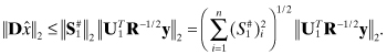
Hence replacing a nonzero element ![]() with zero reduces
with zero reduces ![]() . The fact that certain diagonal elements of S1 are numerically negligible implies that a unique solution to
. The fact that certain diagonal elements of S1 are numerically negligible implies that a unique solution to ![]() does not exist, so an infinite number of solutions are possible.
does not exist, so an infinite number of solutions are possible.
The pseudo-inverse should be used with great caution because it fundamentally changes the nature of the least-squares solution. Rather than accepting that we have no information on a linear combination of states, we are stating that knowledge of that combination of states is perfect. Hence the definition of states included in that linear combination is altered. If the only purpose of the least-squares solution is to obtain a smooth interpolation of noisy data, then use of the pseudo-inverse is justified. However, if the purpose is to predict system variables outside the range of measured conditions (such as prediction past the last measurement time), then use of the pseudo-inverse can produce bad predictions. Likewise if the purpose of least-squares modeling is to determine the values of physical parameters (such as system biases and force model coefficients), then the redefinition of state variables implied by use of the pseudo-inverse is potentially disastrous. Satellite orbit determination is an example where pseudo-inverses should be avoided because typical measurements—such as occasional range and range rates from ground tracking—are not by themselves sufficient to estimate orbit elements. It is only through tracking over a period of time, coupled with a very strong orbital dynamic constraint, that it is possible to obtain a solution. If the model orbit states are redefined by use of a pseudo-inverse, orbit predictions may be poor. Fortunately this problem is seldom encountered because most reasonable orbit determination tracking scenarios result in condition numbers less than 107 (if properly scaled). When larger condition numbers are encountered, iterative methods used to obtain a solution to the nonlinear problem usually do not converge.
When unobservable systems are encountered and the goal of the estimation is other than simply interpolating measurements, it is almost always preferable to either obtain additional measurements or to include prior information on the states (use a Bayesian solution).
The following examples demonstrate problems in using the pseudo-inverse.
Example 5.12: Pseudo-Inverse for Two-State Singular Model
Consider the two-measurement, two-state singular model
![]()
with E[rrT] = I for simplicity. Obviously it is not possible to separately estimate the two states because the mapping to both measurements is identical. The SVD of the measurement matrix H is found to be
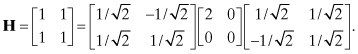
Again for simplicity, we assume that the measurement noise for both measurements is zero, so the measurements are
![]()
Using the pseudo-inverse,
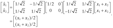
As expected, the estimated states ![]() and
and ![]() are both equal to the average of the measurements. This solution fits the measurements and minimizes the norm
are both equal to the average of the measurements. This solution fits the measurements and minimizes the norm ![]() , but it may be a very poor solution. Suppose that the true state values are x = [1010 − 1010], which give
, but it may be a very poor solution. Suppose that the true state values are x = [1010 − 1010], which give ![]() . In this case the state estimate error is very large, which demonstrates that a minimal norm assumption may produce bad results.
. In this case the state estimate error is very large, which demonstrates that a minimal norm assumption may produce bad results.
As another example, assume that we are given a single noisy measurement, y = h1 − h2 + r, of the difference in height (h1 − h2) for two people. Assume that the actual heights are 69 and 71 inches, so the difference is +2 inches. It can be shown that the pseudo-inverse solution for the two heights are −1 and +1 inches—a physically unrealistic answer. However, if we know that the two people are males living in the United States, then statistical surveys indicate that the mean height should be about 70 inches, with a standard deviation of approximately 3 inches. This can be used as prior information in a Bayesian solution. If the measurement noise standard deviation (![]() ) is 0.1 inch, then the estimated heights of the two people are found to be 69.0006 and 70.9992 inches—a much more accurate answer than when using the pseudo-inverse. Of course the answer would not have been as accurate if the mean height of the two people was not exactly 70 inches, but results would still have been more accurate than the pseudo-inverse solution. Although this example is trivially simple, somewhat similar behavior may be observed for more realistic “unobservable” problems.
) is 0.1 inch, then the estimated heights of the two people are found to be 69.0006 and 70.9992 inches—a much more accurate answer than when using the pseudo-inverse. Of course the answer would not have been as accurate if the mean height of the two people was not exactly 70 inches, but results would still have been more accurate than the pseudo-inverse solution. Although this example is trivially simple, somewhat similar behavior may be observed for more realistic “unobservable” problems.
Example 5.13: Pseudo-Inverse Solution for Polynomial Problem
We return to our polynomial problem of Example 5.4 in which the data span was 0 ≤ t ≤ 1. Let the threshold for computing a pseudo-inverse be ε, where ε ranges from 10−11 to 10−13. That is, for all scaled singular values ε times smaller than the largest singular value, the corresponding diagonal elements of ![]() are set to zero. Figure 5.13 shows the QR and SVD 100-sample RMS solution accuracy,
are set to zero. Figure 5.13 shows the QR and SVD 100-sample RMS solution accuracy,
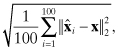
versus polynomial order. The lines labeled
“SVD-RMS-error_epsm11” used ε = 10−11,
“SVD-RMS-error_epsm12” used ε = 10−12, and
“SVD-RMS-error_epsm13” used ε = 10−13
for the SVD solution. Notice that ![]() has lost all accuracy whenever a pseudo-inverse solution is computed because the unobservable linear combinations of
has lost all accuracy whenever a pseudo-inverse solution is computed because the unobservable linear combinations of ![]() have been set to zero.
have been set to zero.
FIGURE 5.13: Least-squares RMS solution accuracy using pseudo-inverse.
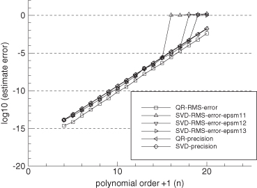
Figure 5.14 shows the 100-sample RMS fit and 1 s measurement (y) prediction accuracy of the QR and pseudo-inverse solutions for n = 20 and ε = 10−12. The QR RMS error is about 0.5 × 10⁻¹⁵ over the first 1 s (the “fit” interval”), and rises to a maximum error of 0.015 at 2.0 s. However, the pseudo-inverse RMS error is about 0.2 × 10⁻¹² over the first second and rises to a maximum of 18.1 at 2.0 s. Although the pseudo-inverse error at 2.0 s is only 2.8 × 10⁻⁵ times the RMS magnitude of the measurement, it is 1200 times larger than the error of the full-rank QR solution. The pseudo-inverse prediction error grows much faster with time than the full-rank prediction, which is a consequence of the constraint imposed by use of the pseudo-inverse. As shown in Figure 5.15, the pseudo-inverse RMS error rises to 78.2 at 2 s when using ε = 10−11. For some problems, changes in ε can result in dramatic changes in errors for predictions outside tested conditions. This is another problem when using pseudo-inverses because the appropriate level of ε is not always obvious.
FIGURE 5.14: RMS QR and pseudo-inverse (ε = 1.e-12) n = 20 polynomial model prediction accuracy versus time.
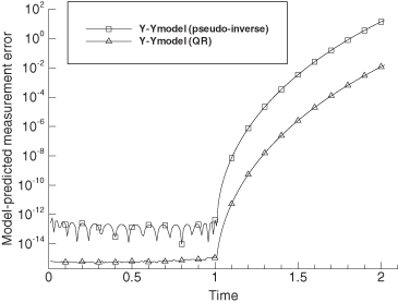
FIGURE 5.15: RMS QR and pseudo-inverse (ε = 1.e-11) n = 20 polynomial model prediction accuracy versus time.
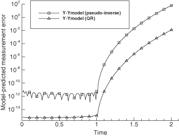
Although not directly relevant to the pseudo-inverse, notice that the estimate errors ![]() from Figure 5.13 are about 0.002 for n = 20 when using the QR algorithm, but the computed model can still fit the measurements to an accuracy of 0.5 × 10⁻¹⁵ over the fit interval (Fig. 5.14).This shows that numerical errors may cause the state estimate to be erroneous, but this does not affect the ability of the model to fit the data.
from Figure 5.13 are about 0.002 for n = 20 when using the QR algorithm, but the computed model can still fit the measurements to an accuracy of 0.5 × 10⁻¹⁵ over the fit interval (Fig. 5.14).This shows that numerical errors may cause the state estimate to be erroneous, but this does not affect the ability of the model to fit the data.
5.9 SUMMARY
The important lessons from this chapter are
1.
The matrix condition number κp(A) = ![]() A
A![]() p
p![]() A−1
A−1![]() p is a measure of the lp-norm relative sensitivity of x to numerical perturbations in A or b for the equation Ax = b, that is,
p is a measure of the lp-norm relative sensitivity of x to numerical perturbations in A or b for the equation Ax = b, that is,
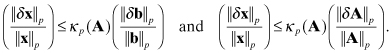
For the l2-norm,

where si are the singular values of A.
2. The Moore-Penrose matrix pseudo-inverse, defined by four properties, is used to compute minimum norm matrix inversions for rectangular and/or singular matrices.
3. Theoretical observability of the measurement equation y = Hx + r is defined by various conditions that all equivalent to the requirement that the rank of the m × n matrix H must be n. This implies that all singular values of H must be greater than zero.
4.
The normal equation ![]() is the most frequently used technique for solving the weighted least-squares problem. The most commonly used solution technique uses Cholesky factorization of HTR−1H = LLT, where L is lower triangular. The solution for
is the most frequently used technique for solving the weighted least-squares problem. The most commonly used solution technique uses Cholesky factorization of HTR−1H = LLT, where L is lower triangular. The solution for ![]() is computed by explicitly or implicitly inverting L. Cholesky factorization is numerically stable, generally does not require pivoting, and provides a metric for determining loss of numeric precision. It can also be easily adapted for partitioned solutions of sparse systems. However, formation of the normal equation doubles the condition number of matrix H, and that can cause a loss of accuracy for poorly conditioned problems.
is computed by explicitly or implicitly inverting L. Cholesky factorization is numerically stable, generally does not require pivoting, and provides a metric for determining loss of numeric precision. It can also be easily adapted for partitioned solutions of sparse systems. However, formation of the normal equation doubles the condition number of matrix H, and that can cause a loss of accuracy for poorly conditioned problems.
5.
The QR factorization (R−1/2H) = TTU, where T is an m × m orthogonal matrix formed using elementary rotations and U is a m × n upper triangular matrix, is a more numerically stable method for solving the least-squares problem. The solution ![]() is obtained by back-solving
is obtained by back-solving ![]() . The condition number of U is the same as that of R−1/2H, so numerical precision is unaltered. The QR factorization is most often computed using Householder transformations or MGS orthogonalization. The MGS method requires slightly more computation, but some results suggest that it is more accurate than Householder transformations. Both methods require approximately twice the flops of normal equation methods, but execution times indicate that it can actually be faster than normal equation methods for some problems. (Note: the QR factorization is usually defined as H = QTR but we have changed the notation [using T and U] to avoid confusion with our previous definitions of Q and R.)
. The condition number of U is the same as that of R−1/2H, so numerical precision is unaltered. The QR factorization is most often computed using Householder transformations or MGS orthogonalization. The MGS method requires slightly more computation, but some results suggest that it is more accurate than Householder transformations. Both methods require approximately twice the flops of normal equation methods, but execution times indicate that it can actually be faster than normal equation methods for some problems. (Note: the QR factorization is usually defined as H = QTR but we have changed the notation [using T and U] to avoid confusion with our previous definitions of Q and R.)
6. The SVD can also be used to solve the least-squares problem. It has the advantages of automatically computing the solution condition number and indicating which linear combinations of states are unobservable, but it can be less accurate than the MGS QR method and requires far more execution time than the QR or normal equation methods. Its primary strength is in determining which states should be included in the system model. If it is to be used operationally for large problems, the QR method should first be used as a “data compression” technique to reduce the system size from m × n to n × n.
7. The normal equations, or equations equivalent to the normal equations, can also be solved using iterative methods. Krylov space methods are particularly useful for solution of large sparse systems. The CGNR and LSQR methods are two iterative methods that solve the least-squares problem without forming the normal equations, but they are both affected by the doubling of the condition number implied by the normal equations. This author has used the CGNR method with success on flow-type problems when preconditioning was used, but on our sample problems without preconditioning, both methods failed completely (without indication of failure) for moderate condition numbers. The LSQR method was generally more accurate than the CGNR method, but also failed more abruptly than CGNR.
8. To use condition numbers as a test for state observability, or equivalently to use the ratio of singular values to determine which linear combinations of variables are unobservable, both row and column scaling of H should be applied before using the SVD. In particular, H′ = R−1/2HD−1 should be used where R−1/2 scales the rows to obtain unit measurement noise variance, and D−1 scales the columns for unit column norms.
9.
When unobservable systems are encountered, it is preferable to either obtain additional measurements or include prior information so that all states are observable. Alternately the pseudo-inverse solution ![]() can be used by replacing diagonals of
can be used by replacing diagonals of ![]() corresponding to negligible-small singular values with zero. However, use of a pseudo-inverse fundamentally alters the definition of estimated states, and can lead to poor predictions of unmeasured conditions, or can result in physically unreasonable state estimates.
corresponding to negligible-small singular values with zero. However, use of a pseudo-inverse fundamentally alters the definition of estimated states, and can lead to poor predictions of unmeasured conditions, or can result in physically unreasonable state estimates.
10. Use of model basis functions that are orthogonal over the measurement data span will eliminate most numerical problems in the least-squares solution because the information matrix HTR−1H will be diagonal. Even when using physically based models, selection of “approximately orthogonal” states can improve the conditioning.