
We started investigating the types of queries we might be interested in at the end of the previous chapter, but we’ve not yet written any routines to help us make sense of the data we’re collecting. In this chapter, we return to Jupyter notebooks, this time as a data analysis tool rather than a prototyping aid.
IPython and Jupyter seamlessly support both synchronous and asynchronous function calls. We have a (mostly) free choice between the two types of API. As the rest of the apd.aggregation package is asynchronous, I recommend that we create some utility coroutines to extract and analyze data.
Query functions
A Jupyter notebook would be able to import and use SQLAlchemy functions freely, but that would require users to understand a lot about the internals of the aggregation system’s data structures. It would effectively mean that the tables and models that we’ve created become part of the public API, and any changes to them may mean incrementing the major version number and documenting changes for end-users.
Instead, let’s create some functions that return DataPoint records for users to interact with. This way, only the DataPoint objects and the function signatures are part of the API that we must maintain for people. We can always add more functions later, as we discover additional requirements.
To begin with, the most important feature that we need is the ability to find data records, ordered by the time they were collected. This lets users write some analysis code to analyze the values of the sensors over time. We may also want to filter this by the sensor type, the deployment identifier, and a date range.
We have to decide what form we want the function to have. Should it return a list or tuple of objects or an iterator? A tuple would allow us to easily count the number of items we retrieved and to iterate over the list multiple times. On the other hand, an iterator would allow us to minimize RAM use, which may help us support much larger data sets, but restricts us to only being able to iterate over the data once. We’ll create iterator functions, as they allow for more efficient code. The iterators can be converted to tuples by the calling code, so our users are able to choose to iterate over a tuple if they prefer.
query.py with a context manager to connect to the database
This function acts as a (synchronous) context manager, setting up a database connection and an associated session and both returning that session and setting it as the value of the db_session_var context variable before entering the body of the associated with block. It also unsets this session, commits any changes, and closes the session when the context manager exits. This ensures that there are no lingering locks in the database, that data is persisted, and that if functions that use the db_session_var variable can only be used inside the body of this context manager.
Jupyter cell to find number of sensor records
We also need to write the function that returns DataPoint objects for the user to analyze. Eventually, we’ll have to deal with performance issues due to processing large amounts of data, but the first code you write to solve a problem should not be optimized, a naïve implementation is both easier to understand and more likely not to suffer from being too clever. We’ll look at some techniques for optimization in the next chapter.
Debugging is twice as hard as writing the code in the first place. Therefore, if you write the code as cleverly as possible, you are, by definition, not smart enough to debug it.
—Brian Kernighan
Python is not the fastest programming language; it can be tempting to write your code to minimize the inherent slowness, but I would strongly recommend fighting this urge. I’ve seen “highly optimized” code that takes an hour to execute, which, when replaced with a naïve implementation of the same logic, takes two minutes to complete.
It isn’t common, but when you make your code more elaborate, you’re making your job harder when it comes to improving it.
If you write the simplest version of a method, you can compare it to subsequent versions to determine if you’re making code faster or just more complex.
Simplest implementation of get_data()
This function gets the session from the context variable set up by with_database(...), builds a query object, and then runs that object’s all method using an executor, giving way to other tasks while the all method runs. Iterating over the query object rather than calling query.all() would cause database operations to be triggered as the loop runs, so we must be careful to only set up the query in asynchronous code and delegate the all() function call to the executor. The result of this is a list of SQLAlchemy’s lightweight result named tuples in the rows variable, which we can then iterate over yielding the matching DataPoint object.
As rows variable contains a list of all the result objects, we know that all the data has been processed by the database and parsed SQLAlchemy in the executor before execution passes back to our get_data() function . This means that we’re using all the RAM needed to store the full results set before the first DataPoint object is available to the end-user. Storing all this data when we don’t know that we need all of it is a little memory and time inefficient, but elaborate methods to paginate the data in the iterator would be an example of premature optimization. Don’t change this from the naïve approach until it becomes a problem.
Jupyter cell to count data points using our helper context manager
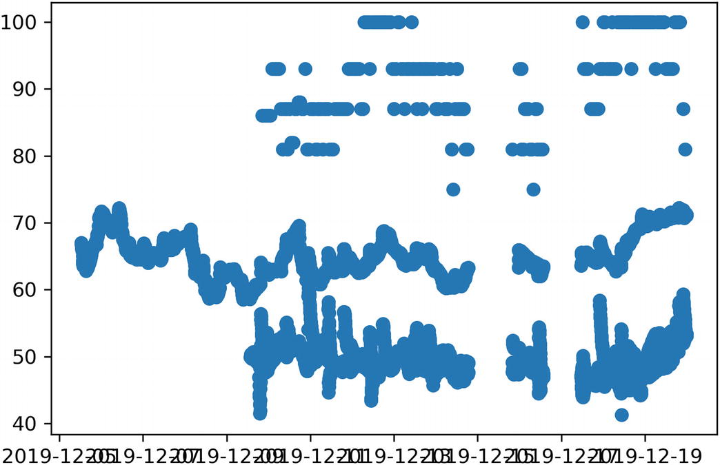
Merely counting the data points isn’t an interesting way of analyzing the data. We can start trying to make sense of the data by plotting values on a scatter plots. Let’s start with a simple sanity check, plotting the value of the RelativeHumidity sensor against date (Listing 9-5). This is a good one to start with, as the stored data is a floating-point number rather than a dictionary-based structure, so we don’t need to parse the values.
The matplotlib library is perhaps the most popular plotting library in Python. Its plot_date(...) function is a great fit for plotting a series of values against time. It takes a list of values for the x axis and a corresponding list of values for the y axis, as well as the style to be used when plotting a point3 and a flag to set which axis contains the date values. Our get_data(...) function doesn’t return what we need for the x and y parameters directly, it returns an async iterator of data point objects.
Relative humidity plotting jupyter cell, with the output chart it generates
Filtering data
Delegating filtering to the get_data function
Plotting all sensor deployments independently
Extended data collection functions for deployment_id filtering
Plotting all deploymens using the new helper functions
This approach allows the end-user to interrogate each deployment individually, so only the relevant data for a combination of sensor and deployment is loaded into RAM at once. It’s a perfectly appropriate API to offer the end-user.
Multilevel iterators
We previously reworked the interface for filtering by sensor name to do the filtering in the database to avoid iterating over unnecessary data. Our new deployment id filter isn’t used to exclude data we don’t need, it’s used to make it easier to loop over each logical group independently. We don’t need to use a filter here, we’re using one to make the interface more natural.
If you’ve worked with the itertools module in the standard library much, you may have used the groupby(...) function . This takes an iterator and a key function and returns an iterator of iterators, the first being the value of the key function and the second being a run of values that match the given result of the key function. This is the same problem we’ve been trying to solve by listing our deployments and then filtering the database query.
The key function given to groupby(...) is often a simple lambda expression, but it can be any function, such as one of the functions from the operator module. For example, operator.attrgetter("deployment_id") is equivalent to lambda obj: obj.deployment_id, and operator.itemgetter(2) is equivalent to lambda obj: obj[2].
Setting up a groupby does not consume the underlying iterable; each item it generates is processed as the groupby is iterated over. To work correctly, the groupby only needs to decide if the current item is in the same group as the previous one or if a new group has started, it doesn’t analyze the iterable as a whole. Items with the same value for the key function are only grouped together if they are a contiguous block in the input iterator, so it’s common to ensure that the underlying iterator is sorted to avoid splitting groups up.
From the output of the print statements, we can see that the groupby only ever pulls one item at a time, but manages the iterators it provides in such a way that looping over the values is natural. Whenever the inner loop requests a new item, the groupby function requests a new item from the underlying iterator and then decides its behavior based on that value. If the key function reports the same value as the previous item, it yields the new value to the inner loop; otherwise, it signals that the inner loop is complete and holds the value until the next inner loop starts.
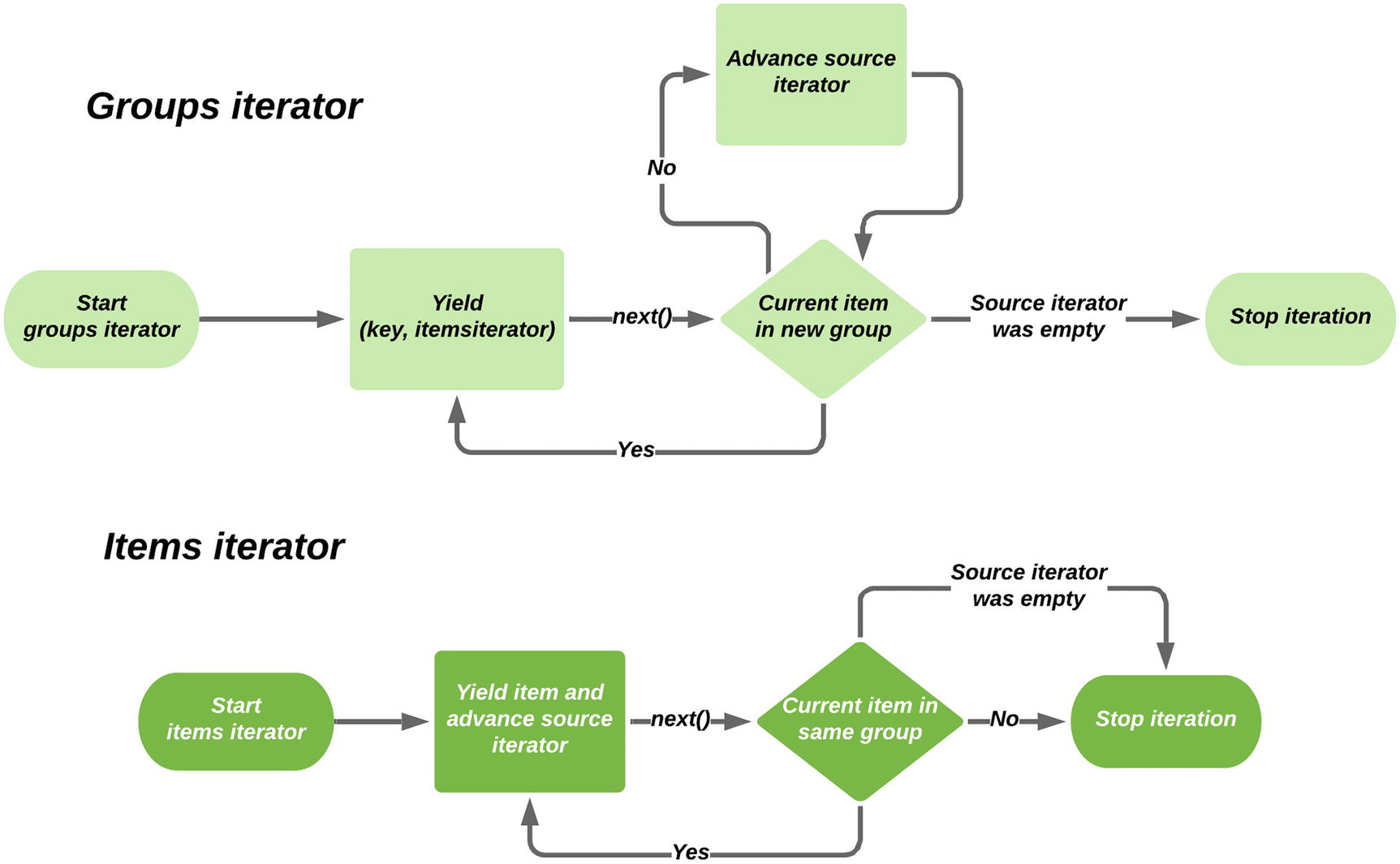
Flow chart demonstrating how groupby works
If we had a standard iterator (as opposed to an asynchronous iterator), we could sort the data by deployment_id and use itertools.groupby(...) to simplify our code to handle multiple deployments without needing to query for the individual deployments. Rather than making a new get_data(...) call for each, we could iterate over the groups and handle the internal iterator in the same way we already do, using list comprehensions and zip(...).
Unfortunately, there is no fully asynchronous equivalent of groupby at the time of writing. While we can write a function that returns an async iterator whose values are UUID and async iterator of DataPoint pairs, there is no way of grouping these automatically.
At the risk of writing clever code, we can write an implementation of groupby that works with asynchronous code ourselves using closures. It would expose multiple iterators to the end-user that work on the same underlying iterator, in just the same way as itertools.groupby(...). It would be better to use a library function for this if one were available.
Each time we find a new value of the key function, we need to return a new generator function that maintains a reference to the underlying source iterator. This way, when someone advances an item iterator, it can choose to either yield the data point it receives or to indicate that it’s the end of the item iterator, as the groupby function does. Equally, if we advance the outer iterator before an item iterator has been consumed, it needs to “fast-forward” through the underlying iterator until the start of a new group is found.
An implementation of get_data_by_deployment that acts like an asynchronous groupby
This uses await data.__anext__() to advance the underlying data iterator, rather than an async for loop, to make the fact that the iterator is consumed in multiple places more obvious.
An implementation of this generator coroutine is in the code for this chapter. I’d encourage you to try adding print statements and breakpoints to it, to help understand the control flow. This code is more complex than most Python code you’ll need to write (and I’d caution you against introducing this level of complexity into production code; having it as a self-contained dependency is better), but if you can understand how it works, you’ll have a thorough grasp on the details of generator functions, asynchronous iterators, and closures. As asynchronous code is used more in production code, libraries to offer this kind of complex manipulation of iterators are sure to become available.
Additional filters
get_data method with sensor, deployment, and date filters
Testing our query functions
The query functions need to be tested, just like any others. Unlike most of the functions we’ve written so far, the query functions take lots of optional arguments that significantly change the output of the returned data. Although we don’t need to test a wide range of values for each filter (we can trust that our database’s query support works correctly), we need to test that each option works as intended.
We need some setup fixtures to enable us to test functions that depend on a database being present. While we could mock the database connection out, I wouldn’t recommend this, as databases are very complex pieces of software and not well suited to being mocked out.
The most common approach to testing database applications is to create a new, empty database and allow the tests to control the creation of tables and data. Some database software, like SQLite, allows for new databases to be created on the fly, but most require the database to be set up in advance.
Given that we’re assuming there’s an empty database available to us, we need a fixture to connect to it, a fixture to set up the tables, and a fixture to set up the data. The connect fixture is very similar to the with_database context manager,5 and the function to populate the database will include sample data that we can insert using db_session.execute(datapoint_table.insert().values(...)).
Database setup fixtures
This gives us an environment where we can write tests that query a database that contains only known values, so we can write meaningful assertions.
Parameterized tests
A parameterized get_data test to verify different filters
The first time this test is run, it has filter={}, num_items_expected=9 as parameters. The second run has filter={"sensor_name": "Test"}, num_items_expected=7, and so on. Each of these test functions will run independently and will be counted as a new passing or failing test, as appropriate.
This will result in six tests being generated, with names like TestGetData.test_iterate_over_items[filter5-2]. This name is based on the parameters, with complex parameter values (like filter) being represented by their name and the zero-based index into the list, and simpler parameters (like num_items_expected) included directly. Most of the time, you won’t need to care about the name, but it can be very helpful to identify which variant of a test is failing.
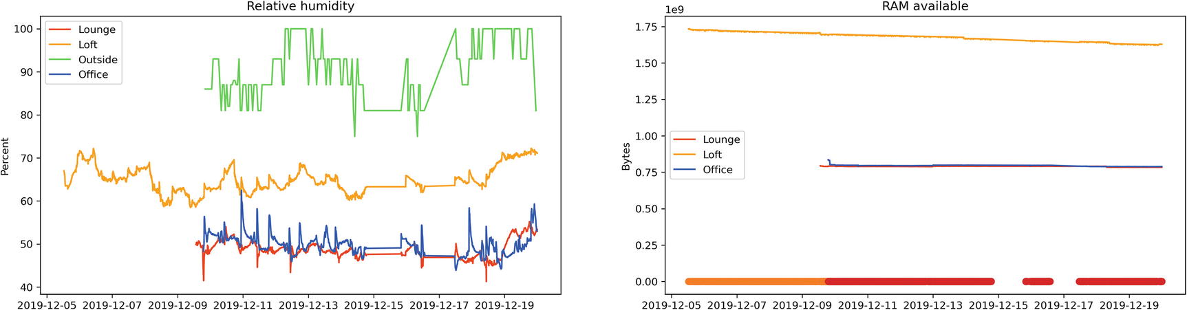
Displaying multiple sensors
We’ve now got three functions that help us connect to the database and iterate over DataPoint objects in a sensible order and with optional filtering. So far we’ve been using the matplotlib.pyplot.plot_dates(...) function to convert pairs of sensor values and dates to a single chart. This is a helper function that makes it easier to generate a plot by making various drawing functions available in a global namespace. It is not the recommended approach when making multiple charts.
We want to be able to loop over each of our sensor types and generate a chart for each. If we were to use the pyplot API, we would be constrained to using a single plot, with the highest values skewing the axes to make the lowest impossible to read. Instead, we want to generate an independent plot for each and show them side by side. For this, we can use the matplotlib.pyplot.figure(...) and figure.add_subplot(...) functions. A subplot is an object which behaves broadly like matplotlib.pyplot but representing a single plot inside a larger grid of plots. For example, figure.add_subplot(3,2,4) would be the fourth plot in a three-row, two-column grid of plots.
Right now, our plot(...) function assumes that the data it is working with is a number, which can be passed directly to matplotlib for display on our chart. Many of our sensors have different data formats though, such as the temperature sensor which has a dictionary of temperature and the unit being used as its value attribute. These different values need to be converted to numbers before they can be plotted.
We can refactor our plotting function out to a utility function in apd.aggregation to vastly simplify our Jupyter notebooks, but we need to ensure that it can be used with other formats of sensor data. Each plot needs to provide some configuration for the sensor to be graphed, a subplot object to draw the plot in, and a mapping from deployment ids to a user-facing name for populating the plot’s legend. It should also accept the same filtering arguments as get_data(...), to allow users to constrain their charts by date or deployment id.
The config data class also needs some string parameters, such as the title of the chart, the axis labels, and the sensor_name that needs to be passed to get_data(...) in order to find the data needed for this chart. Once we have the Config class defined, we can create two config objects that represent the two sensors which use raw floating-point numbers as their value type and a function to return all registered configs.
New config objects and plot function that uses it
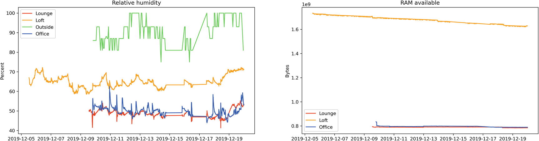
Jupyter cell to plot both Humidity and RAM Available, and their output
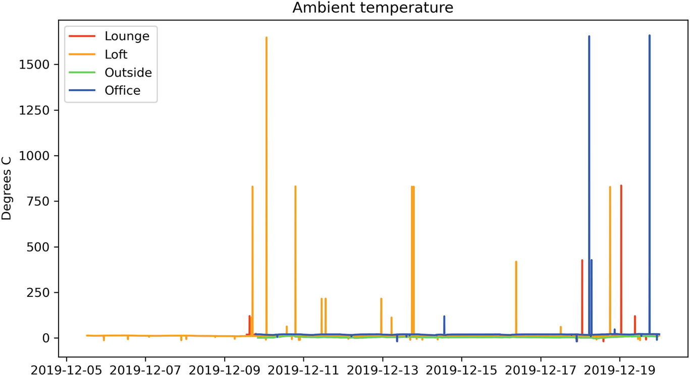
Temperature sensor output with obvious errors skewing the data
Processing data
An advantage of the approach that we’ve taken is that we can perform relatively arbitrary transforms on the data that we’re given, allowing us to discard data points that we consider to be incorrect. It’s often better to discard data when analyzing than during collection, as bugs in the function to check a data point’s validity won’t cause data loss if it’s only checked during analysis. We can always delete incorrect data after the fact, but we can never recollect data that we chose to ignore.
One way of fixing this problem with the temperature sensor would be to make the clean iterator look at a moving window on the underlying data rather than just one DataPoint at a time. This way, it can use the neighbors of a sensor value to discard values that are too different.
The collections.deque type is useful for this, as it offers a structure with an optional maximum size, so we can add each temperature we find to the deque, but when reading it, we only see the last n entries that were added. A deque can have items added or removed from either the left or right edges, so it’s essential to be consistent about adding and popping from the same end when using it as a limited window.
An example implementation of a cleaner function for temperature
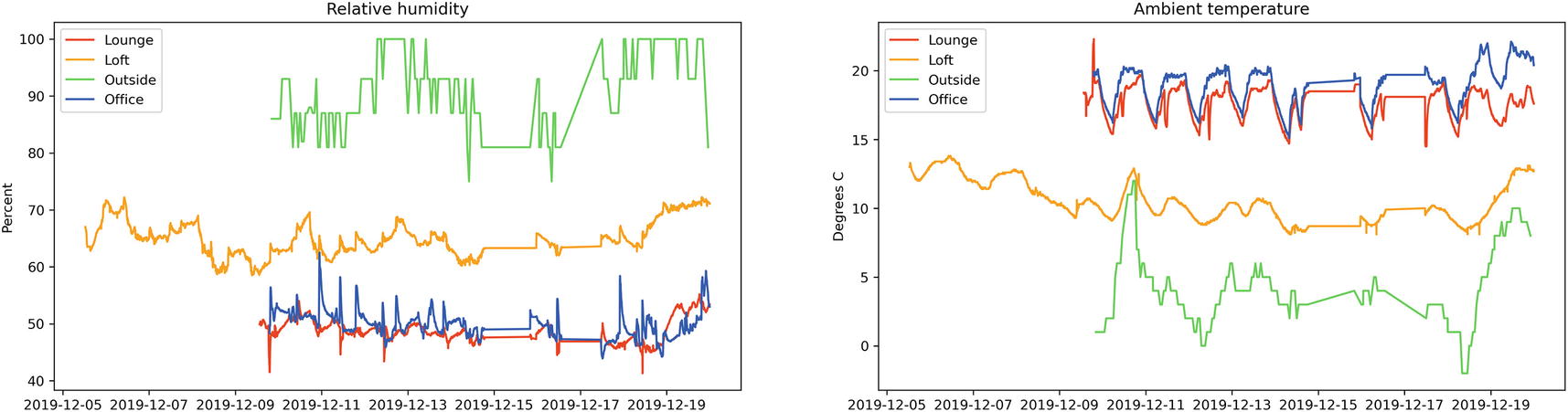
Result of the same data with an appropriate cleaner
The SolarCumulativeOutput sensor returns a number of watt-hours, serialized in the same way as the temperature sensor. If we chart this, we see an upward trending line that moves in irregular steps. It would be much more useful to see the power generated at a moment in time rather than the total up until that time.
To achieve this, we need to convert watt-hours to watts, which means dividing the number of watt-hours by the amount of time between data points.
Write a clean_watthours_to_watts(...) iterator coroutine that keeps track of the last time and watt-hour readings, finds the difference, and then returns watts divided by time elapsed.
The code accompanying this chapter contains a work environment for this exercise, consisting of a test setup with a series of unit tests for this function but no implementation. There is also an implementation of the cleaner as part of the final code for this chapter.
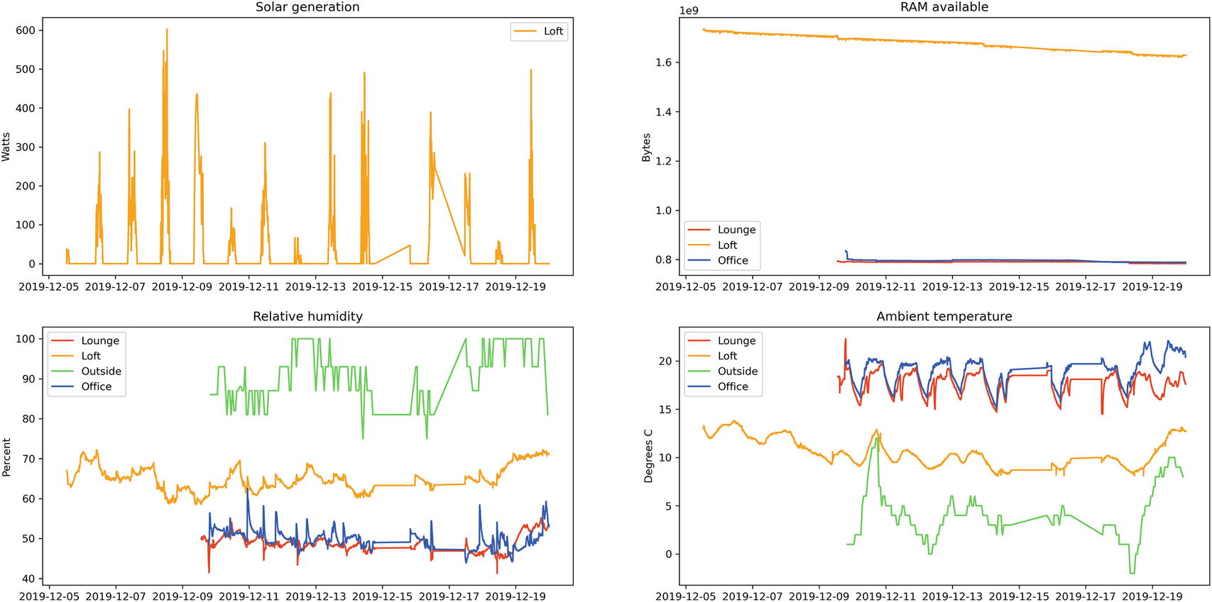
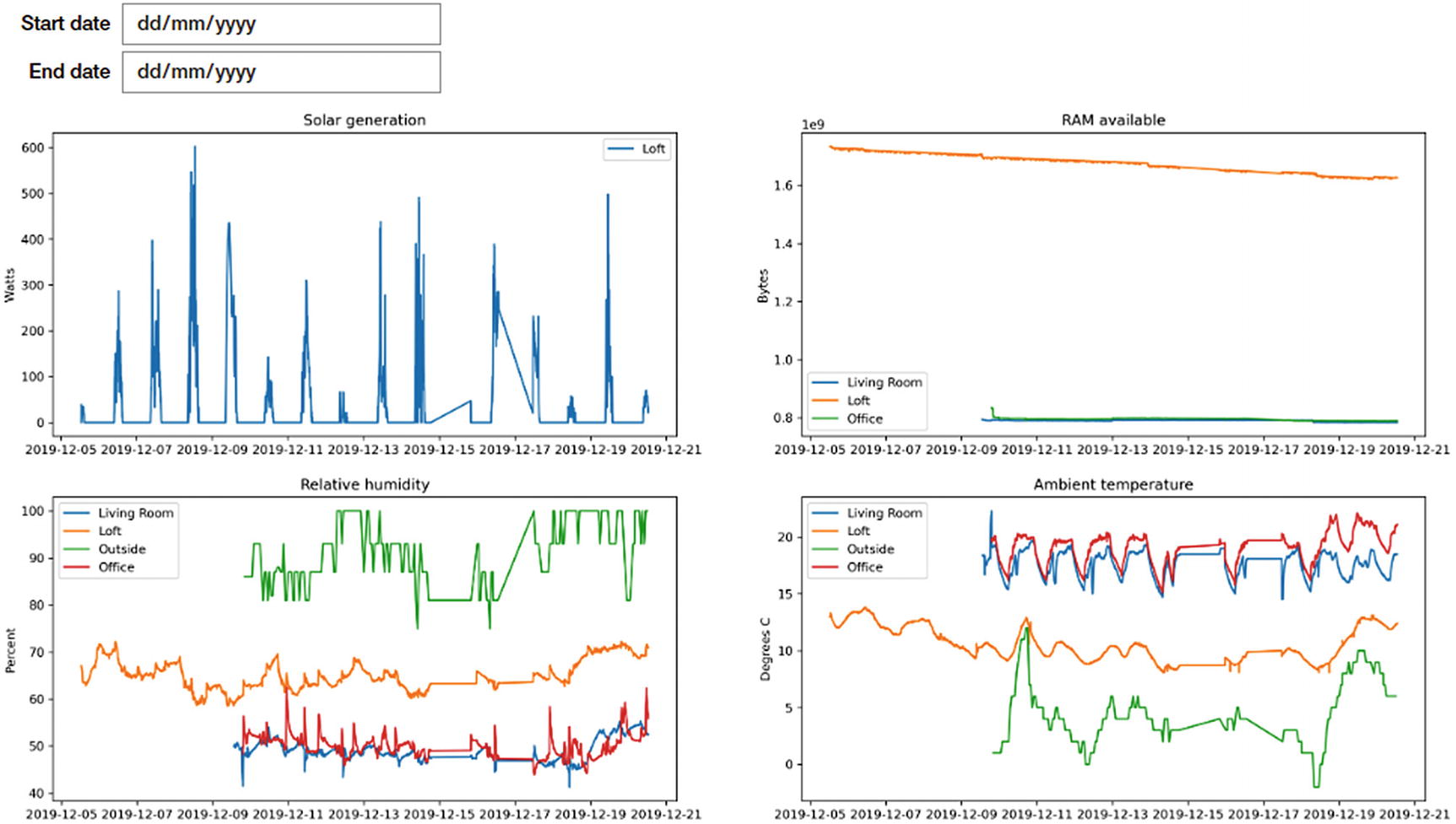
Final Jupyter cell to display 2x2 grid of charts
Interactivity with Jupyter widgets
So far, our code to generate the charts has no interactivity available to the end-user. We are currently displaying all data points ever recorded, but it would be handy to be able to filter to only show a time period without needing to modify the code to generate the chart.
To do this, we add an optional dependency on ipywidgets, using the extras_require functionality of setup.cfg, and reinstall the apd.aggregation package in our environment using pipenv install -e .[jupyter].
With this installed, we can request that Jupyter create interactive widgets for each argument and call the function with the user-selected values. Interactivity allows the person viewing the notebook to choose arbitrary input values without needing to modify the code for the cell or even understand the code.
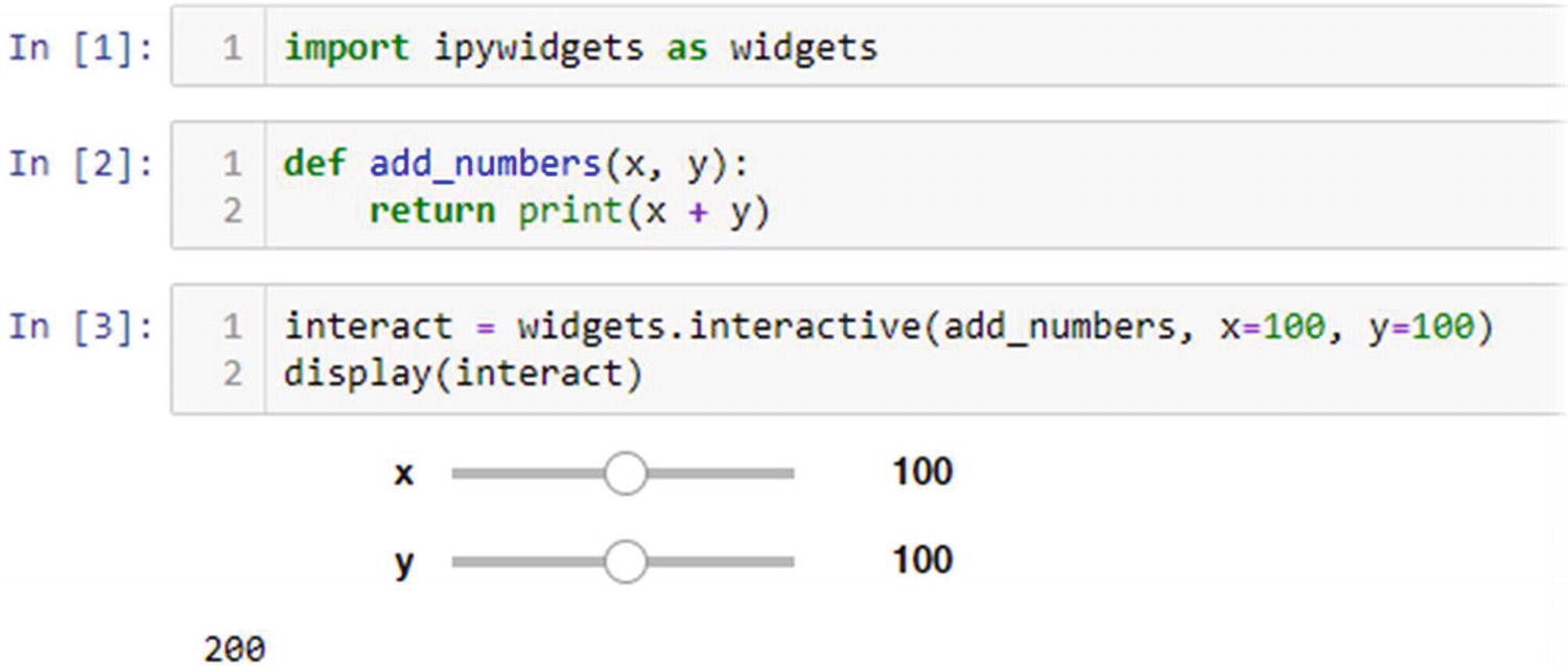
Interactive view of an addition function
Multiply nested synchronous and asynchronous code
We can’t pass coroutines to the interactive(...) function as it’s defined to expect a standard, synchronous function. It's a synchronous function itself, so it’s not even possible for it to await the result of a coroutine call. Although IPython and Jupyter allow await constructs in places where they aren’t usually permitted, this is done by wrapping the cell in a coroutine7 and scheduling it as a task; it is not deep magic that truly marries synchronous and asynchronous code, it’s a hack for convenience.
Our plotting code involves awaiting the plot_sensor(...) coroutine , so Jupyter must wrap the cell into a coroutine. Coroutines can only be called by coroutines or directly on an event loop’s run(...) function, so asynchronous code generally grows to the point that the entire application is asynchronous. It’s a lot easier to have a group of functions that are all synchronous or all asynchronous than it is to mix the two approaches.
We can’t do that here because we need to provide a function to interactive(...), over which we have no control of the implementation. The way we get around this problem is that we must convert the coroutine into a new synchronous method. We don’t want to rewrite all the code to a synchronous style just to accommodate the interactive(...) function, so a wrapper function to bridge the gap is a better fit.
The coroutine requires access to an event loop that it can use to schedule tasks and which is responsible for scheduling it. The existing event loop we have won’t do, as it is busy executing the coroutine that’s waiting for interactive(...) to return. If you recall, it’s the await keyword that implements cooperative multitasking in asyncio, so our code will only ever switch between different tasks when it hits an await expression.
If we are running a coroutine, we can await another coroutine or task, which allows the event loop to execute other code. Execution won’t return to our code until the function that was being awaited has completed execution, but other coroutines can run in the meantime. We can call synchronous code like interactive(...) from an asynchronous context, but that code can introduce blocking. As this blocking is not blocking on an await statement, execution cannot be passed to another coroutine during this period. Calling any synchronous function from an asynchronous function is equivalent to guaranteeing that a block of code does not contain an await statement, which guarantees that no other coroutine’s code will be run.
Until now, we have used the asyncio.run(...) function to start a coroutine from synchronous code and block waiting for its result, but we’re already inside a call to asyncio.run(main()) so we cannot do this again.8 As the interactive(...) call is blocking without an await expression, our wrapper will be running in a context where it’s guaranteed that no coroutine code can run. Although the wrapper function that we use to convert our asynchronous coroutine to a synchronous function must arrange for that coroutine to be executed, it cannot rely on the existing event loop to do this.
Example of calling only synchronous functions from a synchronous context
As this is a coroutine, we can’t pass it directly to the add_number_from_callback(...) function. If we were to try, we’d see Python error TypeError: unsupported operand type(s) for +: 'int' and 'coroutine'.9
The main() task constantly loops over the task.done() check, never hitting an await statement and so never giving way to the async_get_number_from_HTTP_request() task. This function results in a deadlock.
It’s also possible to create blocking asynchronous code with any long-running loop that doesn’t contain an explicit await statement or an implicit one such as async for and async with.
You shouldn’t need to write a loop that checks for another coroutine’s data, as we’ve done here. You should await that coroutine rather than looping. If you do ever need a loop with no awaits inside, you can explicitly give the event loop a chance to switch into other tasks by awaiting a function that does nothing, such as await asyncio.sleep(0), so long as you’re looping in a coroutine rather than a synchronous function that a coroutine called.
We can’t convert the entire call stack to the asynchronous idiom, so the only remaining way around this problem is to start a second event loop, allowing the two tasks to run in parallel. We’ve blocked our current event loop, but we can start a second one to execute the asynchronous HTTP code.
This approach makes it possible to call async code from synchronous contexts, but all tasks scheduled in the main event loop are still blocked waiting for the HTTP response. This only solves the problem of deadlocks when mixing synchronous and asynchronous code; the performance penalty is still in place. You should avoid mixing synchronous and asynchronous code wherever possible. The resulting code is difficult to understand, can introduce deadlocks, and negates the performance benefits of asyncio.
Wrapper function to start a second event loop and delegate new async tasks there
Interactive chart filtering example, with output shown
Tidying up
Genericized versions of the plot functions
Persistent endpoints
The next logical piece of cleanup we could do is to move the configuration of endpoints to a new database table. This would allow us to automatically generate the location_names variable, ensure the colors used on each chart are consistent across invocations, and also let us update all sensor endpoints without having to pass their URLs each time.
To do this, we’ll create a new database table and data class to represent a deployment of apd.sensors. We also need command-line utilities to add and edit the deployment metadata, utility functions to get the data, and tests for all of this.
The changes involved in storing deployments in the database require creating new tables, new console scripts, migrations, and some work on tests.
Deployment object and table that contains id, name, URI, and API key
Command-line scripts to add, edit, and list deployments
Tests for the command-line scripts
Make servers and api_key arguments to collect_sensor_data optional, using the stored values if omitted
Helper function to get a deployment record by its ID
An additional field for the deployment table for the color that should be used to plot its data
Modifications to plot functions to use a deployment’s name and line color directly from its database record
All of these are included in the same implementation that accompanies this chapter.
Charting maps and geographic data
We’ve been focused on xy plots of value against time in this chapter, as it represents the test data we’ve been retrieving. Sometimes we need to plot data against other axes. The most common of these is latitude against longitude, so the plot resembles a map.
Plotting lat/lons using matplotlib, and the resulting chart
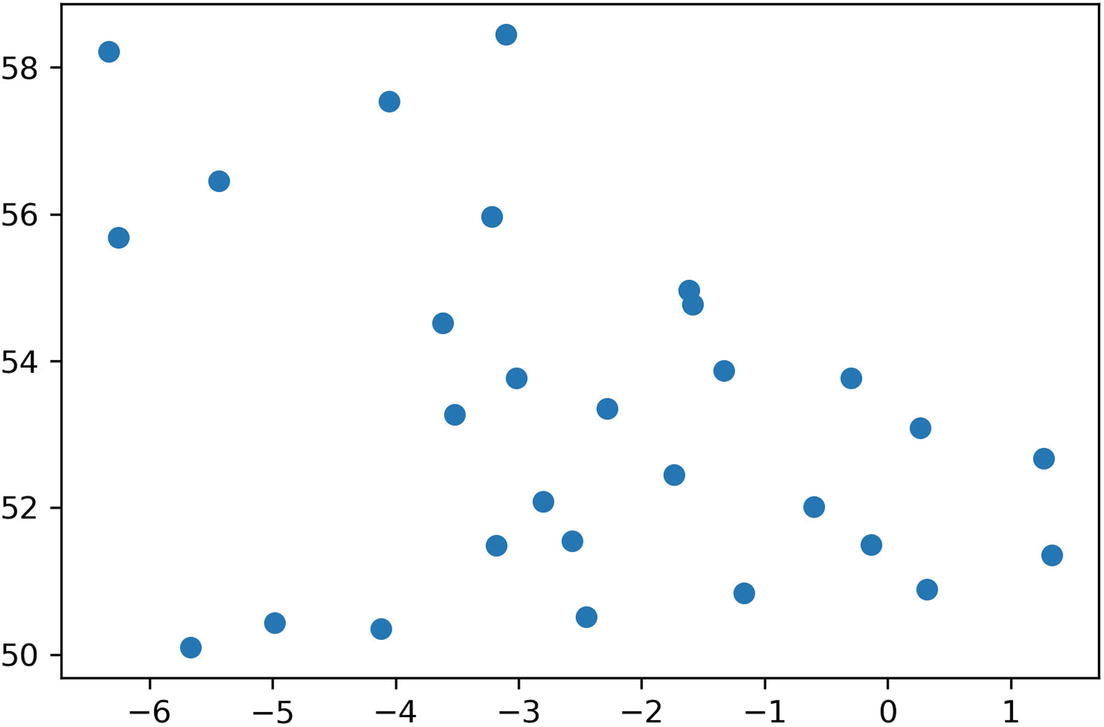

Outline of Great Britain, the island that comprises England, Wales, and Scotland
The distortion is because we’ve plotted this according to the equirectangular map projection, where latitude and longitude are an equally spaced grid that does not take the shape of the earth into account. There is no one correct map projection; it very much depends on what the map’s intended use is.
We need the map to look familiar to most people, who will be very familiar with the outline of whatever country they live in. We want people who look at it to look at the data, not the unusual projection. The most commonly used projection is the Mercator projection, which the OpenStreetMap (OSM) project provides implementations for in many programming languages, including Python.10 The merc_x(...) and merc_y(...) functions to implement the projection won’t be included in the listings, as they’re rather complex mathematical functions.
When drawing maps that show areas of hundreds of square kilometers, it becomes more and more important to use a projection function, but for small-scale maps, it’s possible to provide a more familiar view using the ax.set_aspect(...) function . Changing the aspect ratio moves the point where distortion is at a minimum from the equator to another latitude; it doesn’t correct for the distortion. For example, ax.set_aspect(1.7) would move the point of least distortion to 54 degrees latitude, as 1.7 is equal to 1 / cos(54).
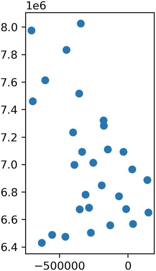
Map using the merc_x and merc_y projections from OSM
New plot types
This only shows us the position of each data point, not the value associated with it. The plotting functions we’ve used so far all plot two values, the x and y coordinates. While we could label the plot points with temperatures, or color code with a scale, the resulting chart isn’t very easy to read. Instead, there are some other plot types in matplotlib that can help us: specifically tricontourf(...). The tricontour family of plotting functions take three-dimensional input of (x, y, value) and interpolate between them to create a plot with areas of color representing a range of values.
Color contours and scatter on the same plot
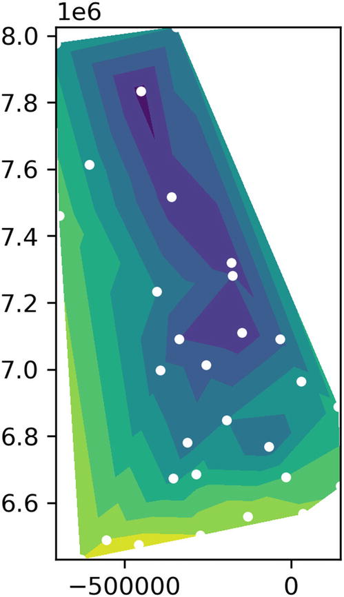
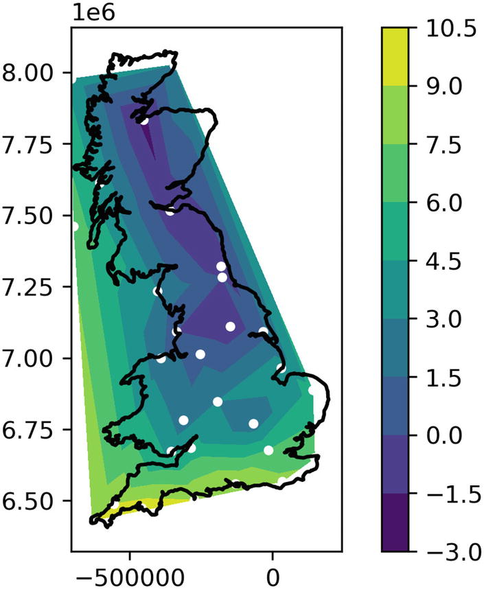
Plot of temperatures around Great Britain on a typical winter’s day
There are lots of GIS libraries for Python and Matplotlib that make more complex maps easier. If you’re planning on drawing lots of maps, I’d encourage you to look at Fiona and Shapely for manipulating points and polygons easily. I strongly recommend these libraries to anyone working with geographic information in Python; they’re very powerful indeed.
The basemap toolkit for matplotlib offers very flexible map drawing tools, but the maintainers have decided against distributing it like a standard Python package so I am unable to recommend it as a general solution to map drawing.
Supporting map type charts in apd.aggregation
We need to make some changes to our config object to support these maps, as they behave differently to all the other plots we’ve made so far. Previously, we’ve iterated over deployments and drawn a single plot for each deployment, representing a single sensor. To draw a map, we’d need to combine two values (coordinate and temperature) and draw a single plot representing all deployments. It’s possible that our individual deployments would move around and would provide a coordinate sensor to record where they were at a given time. A custom cleaner function alone would not be sufficient to combine the values of multiple datapoints.
Backward compatibility in data classes
Our Config object contains a sensor_name parameter , which filters the output of the get_data_by_deployment(...) function call as part of the drawing process. We need to override this part of the system; we no longer want to pass a single parameter to the get_data_by_deployment(...) function; we want to be able to replace the entire call with custom filtering.
Data class with get_data parameter and backward compatibility hook
The __post_init__(...) function is called automatically, passing any InitVar attributes to it. As we are setting get_data in the __post_init__ method, we need to ensure that the data class is not frozen, as this counts as a modification.
This change allows us to change which data is passed to the clean(...) function, but that function still expects to return a time and float tuple to be passed into the plot_date(...) function. We need to change the shape of the clean(...) function.
We will no longer only be using plot_date(...) to draw our points; some types of chart require contours and points, so we must also add another customization point to choose how data are plotted. The new draw attribute of the Config class provides this function.
A generic Config type
It also gives us confidence when we read the code; we know that the argument and return types of functions as specified match up. As this code involves lots of manipulating of data structures into iterators of iterators of tuples (etc.), it is easy to get confused about exactly what’s required. This is a perfect use case for typing hints.
We expect users to be creating custom configuration objects with custom draw and clean methods. Having reliable typing information lets them find subtle errors much more quickly.
The config.get_data(...) and config.draw(...) functions we need to handle our existing two plot types are refactoring of code that we’ve already examined in depth in this chapter, but they are available to view in the code that accompanies this chapter for those who are interested in the details.
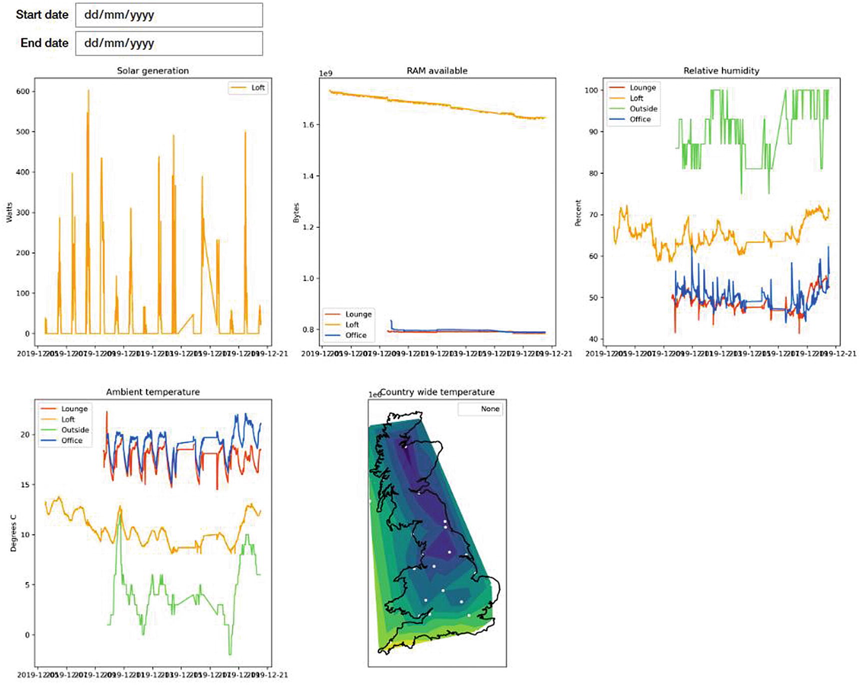
Drawing a custom map using the new configs
Jupyter function to draw a custom map chart along with the registered charts
We wrote a cleaner for the solar generation data to convert it to momentary power instead of cumulative power. This makes it much more evident when power is being generated over time, but it makes understanding the amount generated each day harder.
Write a new cleaner that returns cumulative power per day and a new draw function that displays this as a bar chart.
As always, the code accompanying this chapter includes a starting point and a sample completed version.
Summary
In this chapter, we’ve returned to Jupyter for the purpose that people are most familiar with, rather than purely as a prototyping tool. We’ve also used Matplotlib here, which many users of Jupyter will have come across already. Together, these two make a formidable tool for communicating data analysis outcomes.
We’ve written lots of helper functions to make it easy for people to build custom interfaces in Jupyter to view the data we are aggregating. This has allowed us to define a public-facing API while allowing us lots of flexibility to change the way things are implemented. A good API for end-users is vital for retaining users, so it’s worth spending the time on.
The final version of the accompanying code for this chapter includes all the functions we’ve built up, many of which contain long blocks of sample data. Some of these were too long to include in print, so I recommend that you take a look at the code samples and try them out.
Finally, we’ve looked at some more advanced uses of some technologies we’ve used already, including using the __post_init__(...) hook of data classes to preserve backward compatibility when default arguments do not suffice, and more complex combinations of synchronous and asynchronous code.
Additional resources
Details on the formatting options available on matplotlib charts as well as links to other chart types are available at the matplotlib documentation, at https://matplotlib.org/3.1.1/api/_as_gen/matplotlib.pyplot.plot.html#matplotlib.pyplot.plot.
A testing helper library to manage creating independent postgresql instances is testing.postgresql, available from https://github.com/tk0miya/testing.postgresql.
OpenStreetMap’s page on the Mercator projection, including details of different implementations, is https://wiki.openstreetmap.org/wiki/Mercator.
The Fiona library, for parsing geographic information files in Python, is documented at https://fiona.readthedocs.io/en/latest/README.html.
The Shapely library, for manipulating complex GIS objects in Python, is available at https://shapely.readthedocs.io/en/latest/manual.html. I particularly recommend this one; it’s been useful to me on many occasions.