
There are two main approaches to improving the speed of code: optimizing the code we’ve written and optimizing the control flow of the program to run less code. People often focus on optimizing the code rather than the control flow because it’s easier to make self-contained changes, but the most significant benefits are usually in changing the flow.
Optimizing a function
The first step to optimizing a function is having a good understanding of it’s performance before making any changes. The Python standard library has a profile module to assist with this. Profile introspects code as it runs to build up an idea of the time spent on each function call. The profiler can detect multiple calls to the same function and monitor any functions called indirectly. You can then generate a report that shows the function call chart for an entire run.
The table displayed here shows the number of times a function was invoked (ncalls), the time spent executing that function (tottime), and that total time divided by the number of calls (percall). It also shows the cumulative time spent executing that function and all indirectly called functions, both as a total and divided by the number of calls (cumtime and the second percall). A function having a high cumtime and a low tottime implies that the function itself could not benefit from optimizing, but the control flow involving that function may.
Some IDEs and code editors have built-in support for running profilers and viewing their output. If you’re using an IDE, then this may be a more natural interface for you. The behavior of the profilers is still the same, however.
When running code in a Jupyter notebook, you can also generate the same report using the “cell magic” functionality (Figure 10-1). A cell magic is an annotation on a cell to use a named plugin during execution, in this case a profiler. If you make the first line of your cell %%prun -s cumulative, then once the cell has completed executing, the notebook displays a pop-up window containing a profile report for the whole cell.
The “cell magic” approach is not currently compatible with top-level await support in IPython. If you use the %%prun cell magic, then that cell cannot await a coroutine.
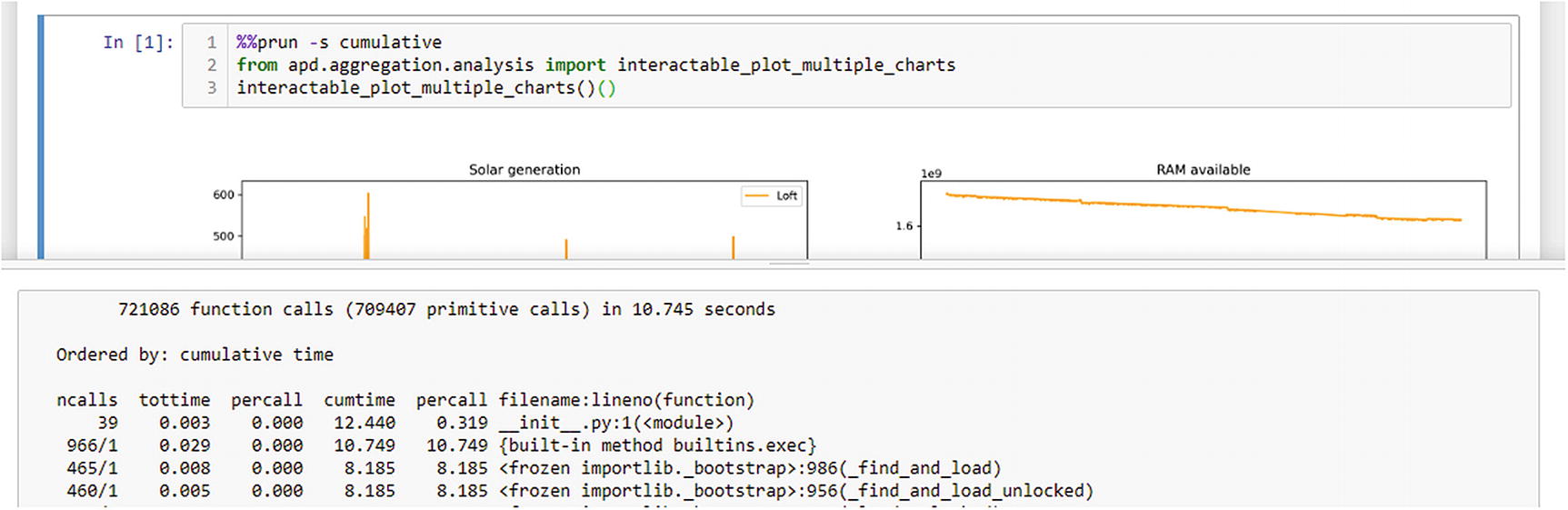
Example of profiling a Jupyter notebook cell
Profiling and threads
The preceding examples generate reports that list lots of threading internal functions rather than our substantive functions. This is because our interactable_plot_multiple_charts(...)(...) function 2 starts a new thread to handle running the underlying coroutines. The profiler does not reach into the started thread to start a profiler, so we only see the main thread waiting for the worker thread to finish.
Example of wrap_coroutine to optionally include profiling
In Listing 10-1, we use the runctx(...) function from the profiler, rather than the run(...) function. runctx(...) allows passing global and local variables to the expression we’re profiling.3 The interpreter does not introspect the string representing the code to run to determine what variables are needed. You must pass them explicitly.
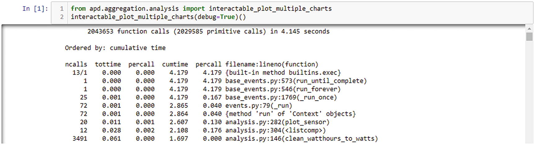
Integrated profiling option being used from Jupyter
It appears that the plot_sensor(...) function is called 20 times, the list comprehension points = [dp async for dp in config.clean(query_results)] is called 12 times, and the clean_watthours_to_watts(...) function is called 3491 times. The huge number of reported calls for the clean function is due to the way the profiler interacts with generator functions. Every time that a new item is requested from the generator, it is classed as a new invocation of the function. Equally, every time an item is yielded, it is classed as that invocation returning. This approach may seem more complex than measuring the time from the first invocation until the generator is exhausted, but it means that the tottime and cumtime totals do not include the time that the iterator was idle and waiting for other code to request the next item. However, it also means that the percall numbers represent the time taken to retrieve a single item, not the time taken for every time the function is called.
Profilers need a function to determine the current time. By default profile uses time.process_time() and cProfile uses time.perf_counter(). These measure very different things. The process_time() function measures time the CPU was busy, but perf_counter() measures real-world time. The real-world time is often called “wall time,” meaning the time as measured by a clock on a wall.
Interpreting the profile report
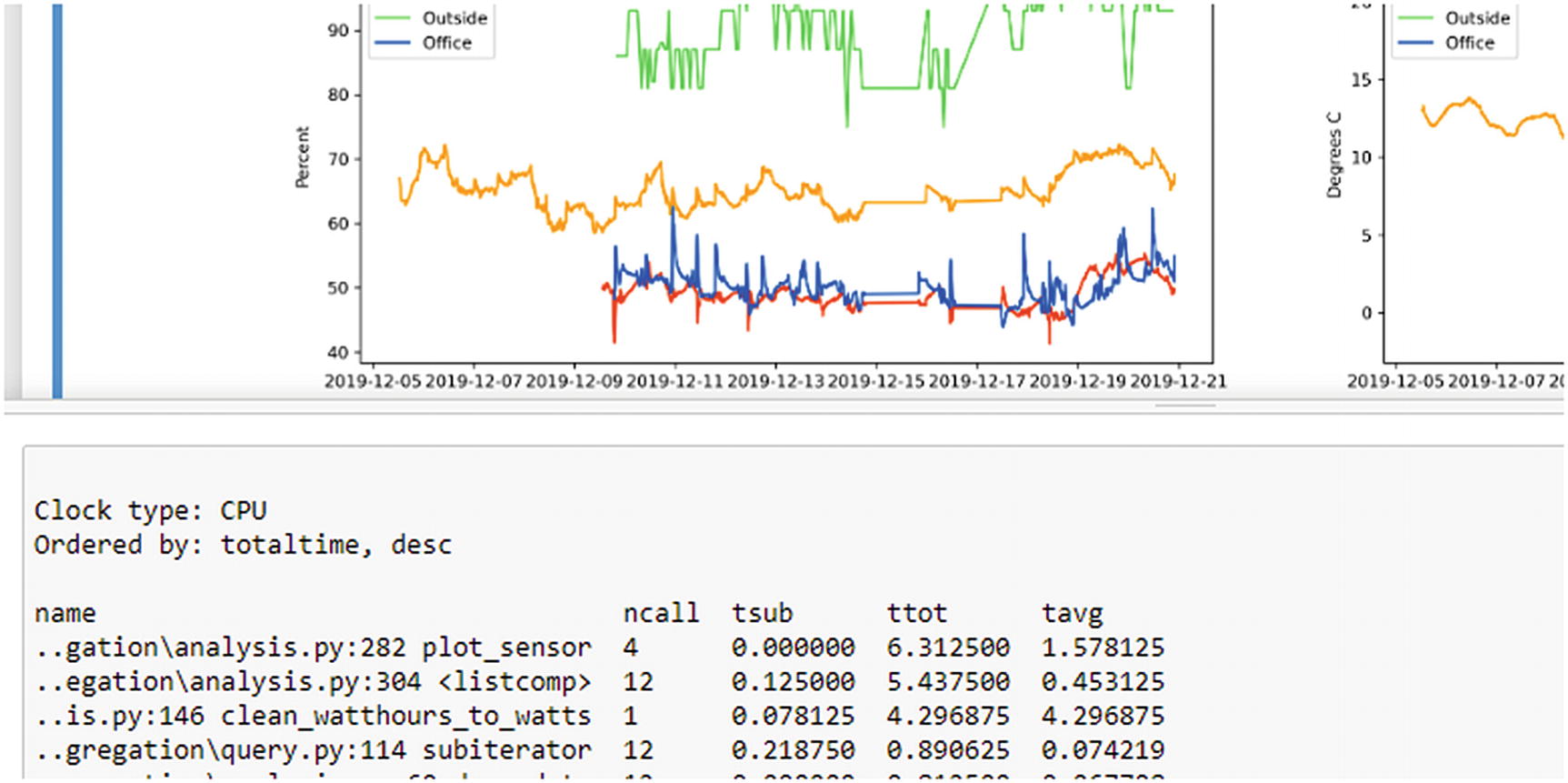
The clean_watthours_to_watts(...) function should draw your eye immediately, as it’s a relatively low-level function with a very high cumtime. This function is being used as a support function to draw one of four charts, but it’s responsible for 65% of the total execution time of plot_sensor(...). This function is where we would start optimization, but if we compare the tottime and the cumtime, we can see that it only spends 2% of the total time in this function.
The discrepancy tells us that it’s not the code we’ve directly written in this function thats introducing the slowdown, it’s the fact that were calling other functions indirectly as part of our implementation of clean_watthours_to_watts(...). Right now, were looking at optimizing functions rather than optimizing execution flow. As optimizing this function requires optimizing the pattern of calling functions out of our control, well pass by it for now. The second half of this chapter covers strategies for improving performance by altering control flow, and well return to fix this function there.
We see that two functions related to the database interface are potential candidates. These are each run over 33,000 times and take less than a tenth of a second total time each, so they are not particularly tempting optimization targets. Still, they’re the highest in terms of tottime of our code, so they represent the best chance we have to do the simple, self-contained type of optimization.
The result here shows that more time was spent in the from_sql_result() function than the previous implementation, but the cumulative time has decreased. This result tells us that the changes we made to from_sql_result() directly caused that function to take longer, but in doing so we changed the control flow to eliminate the call to _asdict() and pass values directly which more than made up for the slowdown we introduced.
In other words, this functions implementation has no definite improvement to performance other than by changing the control flow to avoid code in _asdict(). It also reduces maintainability of the code by requiring us to list the fields in use in multiple places. As a result, well stick with our original implementation rather than the “optimized” version.
There is another potential optimization to class creation, setting a __slots__ attribute on the class, like __slots__ = {"sensor_name", "data", "deployment_id", "id", "collected_at"}. This allows a developer to guarantee that only specifically named attributes will ever be set on an instance, which allows the interpreter to add many optimizations. At the time of writing, there are some incompatibilities between data classes and __slots__ that make it less easy to use, but if you want to optimize instantiation of your objects, then I recommend taking a look.
The same is true of the other two: the subiterator() and list comprehension functions are very minimal; changes to them decrease readability and do not bring substantial performance improvements.
It’s relatively rare for a small, easily understood function to be a candidate for significant performance improvement, as poor performance is often correlated with complexity. If the complexity in your system is due to the composition of simple functions, then performance improvements come from optimizing control flow. If you have very long functions that do complex things, then it’s more likely that significant improvements can come from optimizing functions in isolation.
Other profilers
The profiler that comes with Python is enough to get useful information in most cases. Still, as code performance is such an important topic, there are other profilers available that have unique advantages and disadvantages.
timeit
When called with the default arguments, as previously shown, the output is the number of seconds needed to execute the first argument one million times, measured using the most accurate clock available. Only the first argument (stmt=) is required, which is a string representation of the code to be executed each time. A second string argument (setup=) represents setup code that must be executed before the test starts, and a globals= dictionary allows passing arbitrary items into the namespace of the code being profiled. This is especially useful for passing in the function under test, rather than importing it in the setup= code. The optional number= argument allows us to specify how many times the code should be run, as one million executions is an inappropriate amount for functions that take more than about 50 microseconds to execute.5
Both the string representing the code to test and the setup= strings can be multiline strings containing a series of Python statements. Be aware, however, that any definitions or imports in the first string are run every time, so all setup code should be done in the second string or passed directly as a global.
line_profiler
A commonly recommended alternative profiler is line_profiler by Robert Kern.6 It records information on a line-by-line basis rather than a function-by-function basis, making it very useful for pinpointing where exactly a functions performance issues are coming from.
Unfortunately, the trade-offs for line_profiler are quite significant. It requires modification to your Python program to annotate each function you wish to profile, and while those annotations are in place, the code cannot be run except through the line_profilers custom environment. Also, at the time of writing, it’s not been possible to install line_profiler with pip for approximately two years. Although you will find many people recommending this profiler online, thats partially due to it being available before other alternatives. I would recommend avoiding this profiler unless absolutely necessary for debugging a complex function; you may find it costs you more time to set up than you save in convenience once installed.
yappi
Another alternative profiler is yappi,7 which provides transparent profiling of Python code running across multiple threads and in asyncio event loops. Numbers such as the call count for iterators represent the number of times the iterator is called rather than the number of items retrieved, and no code modifications are needed to support profiling multiple threads.
The disadvantage to yappi is that it’s a relatively small project under heavy development, so you may find it to be less polished than many other Python libraries. I would recommend yappi for cases where the built-in profiler is insufficient. At the time of writing, Id still recommend the built-in profiling tools as my first choice, but yappi is a close second.
Comparison of cProfile and yappi profiling
cProfile using enable/disable API import cProfile profiler = cProfile.Profile() profiler.enable() method_to_profile() profiler.disable() profiler.print_stats() | Yappi-based profiling import yappi yappi.start() method_to_profile() yappi.stop() yappi.get_func_stats().print_all() |
The total times displayed by yappi are significantly higher than those from cProfile in this example. You should only ever compare the times produced by a profiler to results generated on the same hardware with the same tools, as performance can vary wildly8 when profilers are enabled.
Yappi supports filtering stats by function and module out of the box. There is also an option to provide custom filter functions, to determine exactly which code should be displayed in performance reports. There are some other options available; you should check the documentation of yappi to find the recommended way to filter output to only show code you’re interested in.
Jupyter cell for yappi profiling, with part of the Jupyter output shown
None of these three helpers are strictly needed, but they provide for a more user-friendly interface.
Tracemalloc
The profilers we’ve looked at so far all measure the CPU resources needed to run a piece of code. The other primary resource available to us is memory. A program that runs quickly but requires a large amount of RAM would run significantly more slowly on systems that have less RAM available.
Python has a built-in RAM allocation profiler, called tracemalloc. This module provides tracemalloc.start() and tracemalloc.stop() functions to enable and disable to profiler, respectively. A profile result can be requested at any time by using the tracemalloc.take_snapshot() function. An example of using this on our plotting code is given as Listing 10-3.
Example script to debug memory usage after plotting the charts
The documentation in the standard library provides some helper functions to provide for better formatting of the output data, especially the code sample for the display_top(...) function.9
The tracemalloc allocator only shows memory allocations that are still active at the time that the snapshot is generated. Profiling our program shows that the SQL parsing uses a lot of RAM but won’t show our DataPoint objects, despite them taking up more RAM. Our objects are short-lived, unlike the SQL ones, so they have already been discarded by the time we generate the snapshot. When debugging peak memory usage, you must create a snapshot at the peak.
New Relic
If youre running a web-based application, then the commercial service New Relic may provide useful profiling insights.10 It provides a tightly integrated profiling system that allows you to monitor the control flow from web requests, the functions involved in servicing them, and interactions with databases and third-party services as part of the render process.
The trade-offs for New Relic and it’s competitors are substantial. You gain access to an excellent set of profiling data, but it doesnt fit all application types and costs a significant amount of money. Besides, the fact that the actions of real users are used to perform the profiling means that you should consider user privacy before introducing New Relic to your system. That said, New Relics profiling has provided some of the most useful performance analyses Ive seen.
Optimizing control flow
More commonly, it’s not a single function that is the cause of performance problems within a Python system. As we saw earlier, writing code in a naïve way generally results in a function that cannot be optimized beyond changing what it’s doing.
In my experience, the most common source of low performance is a function that calculates more than it needs to. For example, in our first implementations of features to get collated data, we did not yet have database-side filtering, so we added a loop to filter the data we want from the data thats not relevant.
Filtering the input data later doesnt just move workaround; it can increase the total amount of work being done. In this situation, the work done is loading data from the database, setting up DataPoint records, and extracting the relevant data from those records. By moving the filtering from the loading step to the extracting step, we set up DataPoint records for objects that we know we dont care about.
The time taken by a function is not always directly proportional to the size of the input, but it’s a good approximation for functions that loop over the data once. Sorting and other more complex operations behave differently.
The relationship between how long functions take (or how much memory they need) and their input size is called computational complexity. Most programmers never need to worry about the exact complexity class of functions, but it’s worth being aware of the broad-strokes differences when optimizing your code.
You can estimate the relationship between input size and time using the timeit function with different inputs, but as a rule of thumb, it’s best to avoid nesting loops within loops. Nested loops that always have a very small number of iterations are okay, but looping over user input within another loop over user input results in the time a function takes increasing rapidly11 as the amount of user input increases.
The longer a function takes for a given input size, the more important it is to minimize the amount of extraneous data it processes.
In Figure 10-3, the horizontal axis maps to the time taken and the vertical axis to the amount of input a stage in the pipeline has to process. The width of a step, and therefore the time it takes to process, is proportional to the amount of data that it is processing.
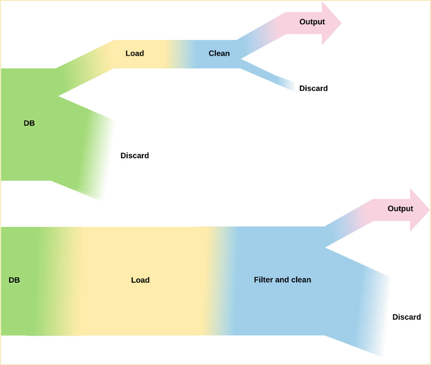
Diagram of the size of data set for code that filters in the database vs. filtering during cleaning
There are two places that we discard data: when we are finding only the data for the sensor in question and when discarding invalid data. By moving the sensor filter to the database, we reduce the amount of work done in the load step and therefore the amount of time needed. We are moving the bulk of the filtering, with the more complex filtering for removing invalid data still happening in the clean step. If we could move this filtering to the database, it would further decrease the time taken by the load step, albeit not as much.
Jupyter cell to profile a single chart, filtering in SQL
Jupyter cell to profile drawing the same chart but without any database filtering
Visualizing profiling data
Complex iterator functions are hard to profile, as seen with clean_temperature_fluctuations(...) listing it’s tsub time as exactly zero. It is a complex function that calls other methods, but for it to spend exactly zero time must be a rounding error. Profiling running code can point you in the right direction, but you’ll only ever get indicative numbers from this approach. It’s also hard to see how the 0.287 seconds total time breaks down by constituent functions from this view.
Both the built-in profile module and yappi support exporting their data in pstats format, a Python-specific profile format that can be passed to visualization tools. Yappi also supports the callgrind format from the Valgrind profiling tool.
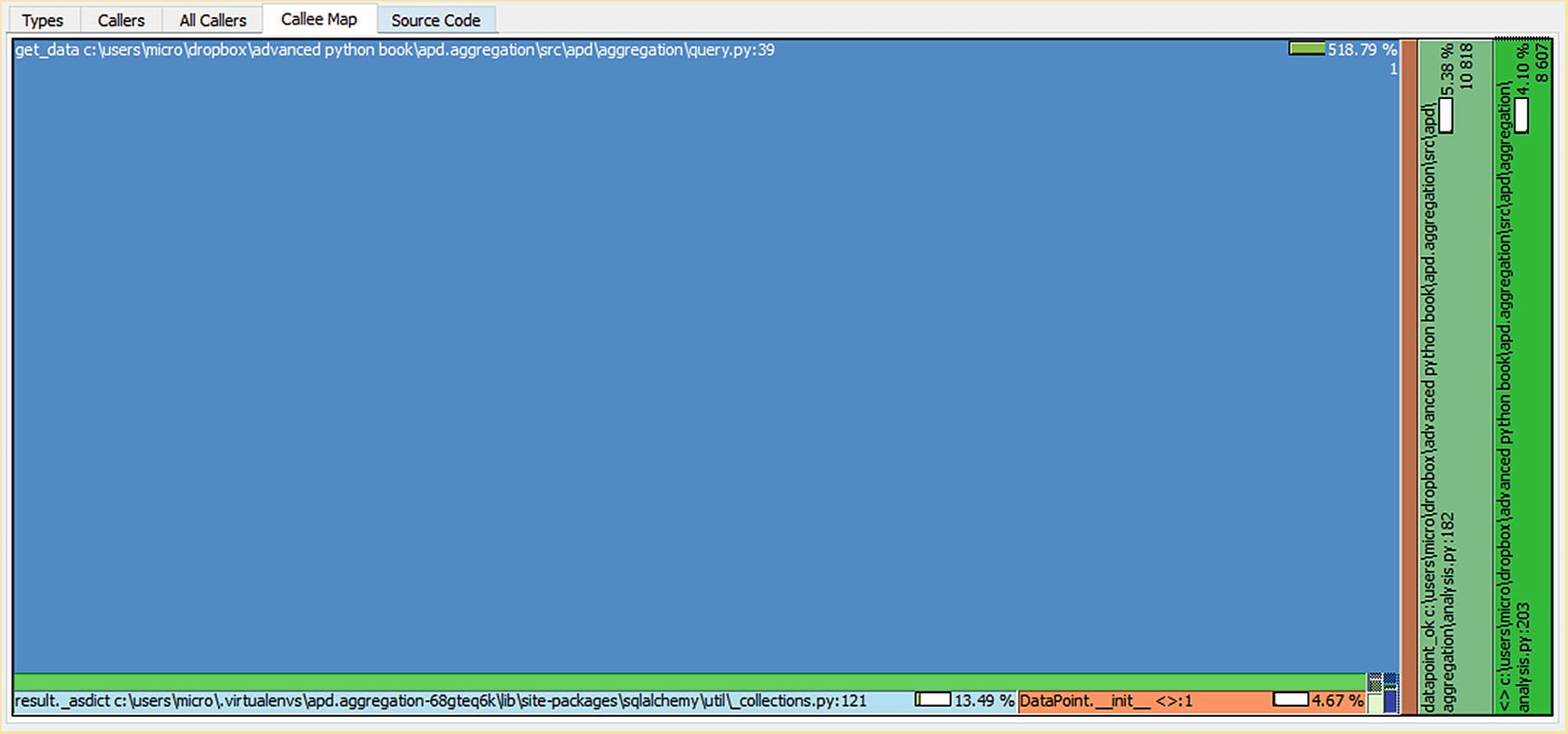
Call chart for clean_temperature_fluctuations when filtering data in the database
You may be surprised to learn that get_data(...) is not only present in this chart but is by far the largest single block. The clean_temperature_fluctuations(...) function doesnt appear to call the get_data(...) function, so it’s not immediately obvious why this function should account for most of the time taken.
Iterators make reasoning about call flow difficult, as when you pull an item from an iterable in a loop, it doesnt look like a function call. Under the hood, Python is calling youriterable.__next__() (or youriterable.__anext__()), which passes execution back to the underlying function, completing the previous yield. A for loop can, therefore, cause any number of functions to be called, even if it’s body is empty. The async for construction makes this a bit clearer, as it is explicitly saying that the underlying code may await. It wouldnt be possible for the underlying code to await unless control was passing to other code rather than just interacting with a static data structure. When profiling code that consumes iterables, you will find the underlying data generation functions called by the functions that use the iterable are present in the output.
Pair of functions for consuming iterators in place
We can simplify this using the functools module in the standard library, specifically the @singledispatch decorator. Back in the second chapter, we looked at Python’s dynamic dispatch functionality, which allows a function to be looked up by the class to which it’s attached. We’re doing something similar here; we have a pair of functions that are associated with an underlying data type, but these data types aren’t classes we’ve written. We have no control over what functions are attached to them, as the two types are features of the core language rather than classes we’ve created and can edit.
Pair of functions for consuming iterators in place with single dipatch
The functions passed to register must have a type definition or a type passed to the register function itself. We’ve used collections.abc.AsyncIterator rather than typing.AsyncIterator as the type here, as the type must be runtime checkable. This means that @singledispatch is limited to dispatching on concrete classes or abstract base classes.
The typing.AsyncIterator type is a generic type: we can use typing.AsyncIterator[int] to mean an iterator of ints. This is used by mypy for static analysis , but isn’t used at runtime. There’s no way that a running Python program can know if an arbitrary async iterator is a typing.AsyncIterator[int] iterator without consuming the whole iterator and checking its contents.
collections.abc.AsyncIterator makes no guarantees about the contents of the iterator, so it is similar to typing.AsyncIterator[typing.Any], but as it is an abstract base class, it can be checked with isinstance(...) at runtime.
Caching
Another way that we can improve performance is to cache the results of function calls. A cached function call keeps a record of past calls and their results, to avoid computing the same value multiple times. So far, we’ve been plotting temperatures using the centigrade temperature system, but a few countries have retained the archaic Fahrenheit system of measurement. It would be nice if we could specify which temperature system we want to use to display our charts, so users can choose the system with which they are most familiar.
Typed conversion functions
We have used t.TypeVar(...) before, to represent a placeholder in a generic type, such as when we defined the draw(...) function in our config class. We had to use T_key and T_value type variables there because some functions in the class used a tuple of key and value and others used a pair of key and value iterables.
If you’re expecting there to be lots of different types of cleaned/cleaner types, then this approach is a bit clearer than explicitly assigning the full types to every function.
The cleaner functions that return this data are a bit more complicated, as mypy’s ability to infer the use of generic types in callables has limits. To create complex aliases for callable and class types (as opposed to data variables), we must use the protocol feature. A protocol is a class that defines attributes that an underlying object must possess to be considered a match, very much like a custom abstract base class’s subclasshook, but in a declarative style and for static typing rather than runtime type checking.
The covariant= argument in the TypeVar is a new addition, as is the _co suffix we used for the variable name. Previously, our type variables have been used to define both function parameters and function return values. These are invariant types: the type definitions must match exactly. If we declare a function that expects a Sensor[float] as an argument, we cannot pass a Sensor[int]. Normally, if we were to define a function that expects a float as an argument, it would be fine to pass an int.
This is because we haven’t given mypy permission to use it’s compatibility checking logic on the constituent types of the Sensor class. This permission is given with the optional covariant= and contravariant= parameters to type variables. A covariant type is one where the normal subtype logic applies, so if the Sensor’s T_value were covariant, then functions that expect Sensor[float] can accept Sensor[int], in the same way that functions that expect float can accept int. This makes sense for generic classes that have functions that provide data to the function they’re passed to.
A contravariant type (usually named with the _contra suffix) is one where the inverse logic holds. If Sensor’s T_value were contravariant, then functions that expect Sensor[float] cannot accept Sensor[int], but they must accept things more specific than float, such as Sensor[complex]. This is useful for generic classes that have functions that consume data from the function they’re passed to.
We’re defining a protocol that provides data,13 so a covariant type is the natural fit. Sensors are simultaneously a provider (sensor.value()) and a consumer (sensor.format(...)) of data and so must be invariant.
Mypy detects the appropriate type of variance when checking a protocol and raises an error if it doesn’t match. As we are defining a function that provides data, we must set covariant=True to prevent this error from showing.
The bound= parameter specifies a minimum specification that this variable can be inferred to be. As this is specified to be Cleaned, T_cleaned_co is only valid if it can be inferred to be a match to Cleaned[Any, Any]. CleanerFunc[int] is not valid, as int is not a subtype of Cleaned[Any, Any]. The bound= parameter can also be used to create a reference to the type of an existing variable, in which case it allows the definition of types that follow the signature of some externally provided function.
Protocols and type variables are powerful features that can allow for much simpler typing, but they can also make code look confusing if they’re overused. Storing types as variables in a module is a good middle ground, but you should ensure that all typing boilerplate is well commented and perhaps even placed in a utility file to avoid overwhelming new contributors to your code.
Jupyter cell to generate a single chart showing temperature in degrees F
The convert_temperature(...) function itself is invoked 8455 times, although datapoint_ok(...) is invoked 10818 times. This tells us that by filtering through datapoint_ok(...) and the cleaning function before converting the temperature, we’ve avoided 2363 calls to convert_temperature(...) for data we dont need to know about to draw the current chart. However, the calls we did make still took 6.58 seconds, tripling the total time taken to draw this chart. This is excessive.
We can optimize this function by reimplementing it to remove the dependency on pint and therefore reducing the overhead involved. If convert_temperature(...) were a simple arithmetic function, the time taken would be reduced to 0.02 seconds, at the expense of a lot of flexibility. This is fine for a simple conversion where both units are needed; pint excels in situations where the exact conversion isnt known ahead of time.
A simple manual cache
A caches efficiency14 is usually measured by hit rate. If our data set were to be [21.0, 21.0, 21.0, 21.0], then our hit rate would be 75% (miss, hit, hit, hit). If it were [1, 2, 3, 4], then the hit rate would drop to zero. The preceding cache implementation assumes a reasonable hit rate, as it makes no effort to evict unused values from it’s cache. A cache is always a trade-off between the extra memory used and time saving it allows. The exact tipping point where it becomes worth it depends on the size of the data being stored and your individual requirements for memory and time.
A common strategy for evicting data from a cache is that of an LRU (least recently used) cache. This strategy defines a maximum cache size. If the cache is full, when a new item is to be added, it replaces the one that has gone the longest without being accessed.
The functools module provides an implementation of an LRU cache as a decorator, which makes it convenient for wrapping our functions. We can also use it to create cached versions of existing functions by manually wrapping a function in an LRU cache decorator.
An LRU cache can be used if a function takes only hashable types as arguments. If a mutable type (such as a dictionary, list, set, or data class without frozen=True) is passed to a function wrapped in an LRU cache, a TypeError will be raised.
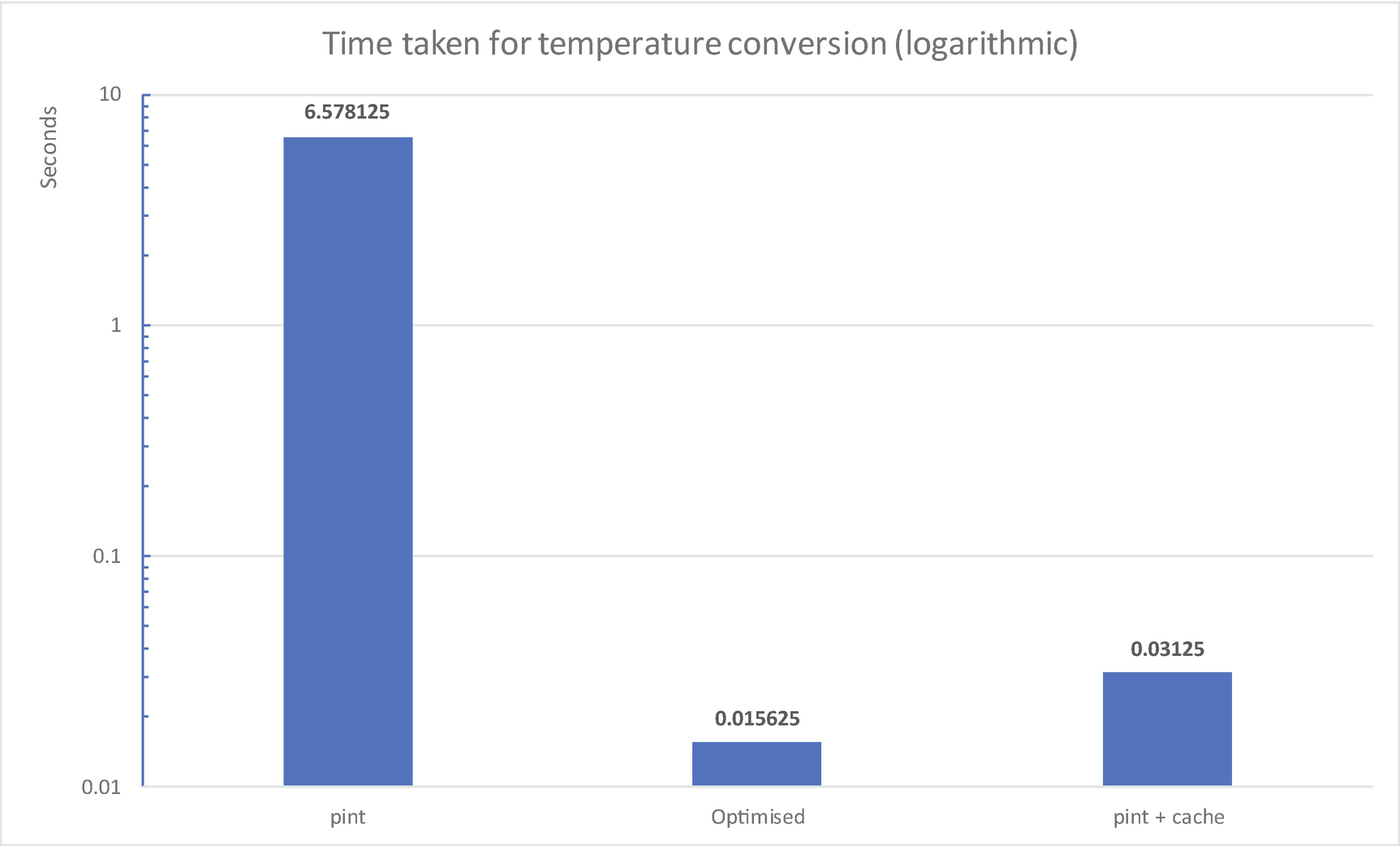
Summary of performance of three approaches
Rewriting the function to avoid using pint would still result in performance improvement, but caching the results provides an improvement of approximately the same magnitude for a much smaller change, both in terms of lines of code and conceptually.
As always, there is a balancing act at play here. It’s likely that people would want temperature only in degrees Celsius or degrees Fahrenheit, so a conversion function that only provides those two is probably good enough. The conversion itself is straightforward and well understood, so the risk of introducing bugs is minimal. More complex functions may not be so easy to optimize, which makes caching a more appealing approach. Alternatively, they may process data that implies a lower hit rate, making refactoring more appealing.
The benefit of the @lru_cache decorator isnt in the inherent efficiency of the cache (its a rather bare-bones cache implementation), but in that it’s easy to implement for Python functions. The implementation of a function decorated with a cache can be understood by everyone who needs to work with it as they can ignore the cache and focus on the function body. If youre writing a custom caching layer, for example, using systems like Redis as the storage rather than a dictionary, you should build your integration such that it doesnt pollute the decorated code with cache-specific instructions.
Cached properties
Another caching decorator available in the functools module is @functools.cached_property. This type of cache is more limited than an LRU cache, but it fits a use case thats common enough that it warrants inclusion in the Python standard library. A function decorated with @cached_property acts in the same way as one decorated with @property, but the underlying function is called only once.
The first time that the program reads the property, it is transparently replaced with it’s result of the underlying function call.15 So long as the underlying function behaves predictably and without side effects,16 a @cached_property is indistinguishable from a regular @property . Like @property, this can only be used as an attribute on a class and must take the form of a function that takes no arguments except for self.
The @property line in the DHTSensor class can be replaced with @cached_property to cache the sensor object between invocations. Adding a cache here doesnt impact the performance of our existing code, as we do not hold long-lived references to sensors and repeatedly query their value, but any third-party users of the sensor code may find it to be an advantage.
At the start of this chapter, we identified the clean_watthours_to_watts(...) functions as the most in need of optimization. On my test data set, it was adding multiple seconds to the execution run.
In the accompanying code to this chapter, there are some extended tests to measure the behavior of this function and it’s performance. Tests to validate performance are tricky, as they are usually the slowest tests, so I don’t recommend adding them as a matter of course. If you do add them, make sure to mark them as such so that you can skip them in your normal test runs.
Modify the clean_watthours_to_watts(...) function so that the test passes. You will need to achieve a speedup of approximately 16x for the test to pass. The strategies discussed in this chapter are sufficient to achieve a speedup of about 100x.
Summary
The most important lesson to learn from this chapter is that no matter how well you understand your problem space, you should always measure your performance improvements, not just assume that they are improvements. There is often a range of options available to you to improve performance, some of which are more performant than others. It can be disappointing to think of a clever way of making something faster only to learn that it doesnt actually help, but it’s still better to know.
The fastest option may require more RAM than can reasonably be assumed to be available, or it may require the removal of certain features. You must consider these carefully, as fast code that doesnt do what the user needs is not useful.
The two caching functions in functools are to be aware of for everyday programming. Use @functools.lru_cache for functions that take arguments and @functools.cached_property for calculated properties of objects that are needed in multiple places.
If your typing hints start to look cumbersome, then you should tidy them up. You can assign types to variables and represent them with classes like TypedDict and Protocol, especially when you need to define more complex structured types. Remember that these are not for runtime type checking and consider moving them to a typing utility module for clearer code. This reorganization has been applied in the sample code for this chapter.
Additional resources
If youre interested in the logic of the different variances used in typing, Id recommend reading up on the Liskov Substitution Principle. The Wikipedia page at https://en.wikipedia.org/wiki/Liskov_substitution_principle is a good starting place, especially for links to computer science course materials on the subject.
More details on how mypy handles protocols and some advanced uses, such as allowing limited runtime checking of protocol types, are found at https://mypy.readthedocs.io/en/stable/protocols.html.
Beaker (https://beaker.readthedocs.io/en/latest/) is a caching library for Python that supports various back-end storages. It’s especially aimed at web applications, but can be used in any type of program. It’s useful for situations where you need multiple types of cache for different data.
The two third-party profiles we’ve used in this chapter are https://github.com/rkern/line_profiler and https://github.com/sumerc/yappi.
Documentation on how to customize the timer used with the built-in profiling tools is available in the standard librarys docs at https://docs.python.org/3/library/profile.html#using-a-custom-timer.