
In this chapter, we will explore the different ways that you can experiment with what different Python functions do and when is an appropriate time to use those different options. Using one of those methods, we will build some simple functions to extract the first pieces of data that we will be aggregating and see how to build those into a simple command-line tool.
Prototyping in Python
During any Python project, from something that you’ll spend a few hours developing to projects that run for years, you’ll need to prototype functions. It may be the first thing you do, or it may sneak up on you mid-project, but sooner or later, you’ll find yourself in the Python shell trying code out.
There are two broad approaches for how to approach prototyping: either running a piece of code and seeing what the results are or executing statements one at a time and looking at the intermediate results. Generally speaking, executing statements one by one is more productive, but at times it can seem easier to revert to running a block of code if there are chunks you’re already confident in.
The Python shell (also called the REPL for Read, Eval, Print, Loop) is most people’s first introduction to using Python. Being able to launch an interpreter and type commands live is a powerful way of jumping right into coding. It allows you to run commands and immediately see what their result is, then adjust your input without erasing the value of any variables. Compare that to a compiled language, where the development flow is structured around compiling a file and then running the executable. There is a significantly shorter latency for simple programs in interpreted languages like Python.
Prototyping with the REPL
The strength of the REPL is very much in trying out simple code and getting an intuitive understanding of how functions work. It is less suited for cases where there is lots of flow control, as it isn’t very forgiving of errors. If you make an error when typing part of a loop body, you’ll have to start again, rather than just editing the incorrect line. Modifying a variable with a single line of Python code and seeing the output is a close fit to an optimal use of the REPL for prototyping.
For example, I often find it hard to remember how the built-in function filter(...) works. There are a few ways of reminding myself: I could look at the documentation for this function on the Python website or using my code editor/IDE. Alternatively, I could try using it in my code and then check that the values I got out are what I expect, or I could use the REPL to either find a reference to the documentation or just try the function out.
The built-in function help(...) is invaluable when trying to understand how functions work. As filter has a clear docstring, it may have been even more straightforward to call help(filter) and read the information. However, when chaining multiple function calls together, especially when trying to understand existing code, being able to experiment with sample data and see how the interactions play out is very helpful.
fizzbuzz.py – a typical implementation
Every time we do this, we are having to reenter code that we entered before, sometimes with small changes, sometimes verbatim. These lines are not editable once they’ve been entered, so any typos mean that the whole loop needs to be retyped.
You may decide to prototype the body of the loop rather than the whole loop, to make it easier to follow the action of the conditions. In this example, the values of n from 1 to 14 are correctly generated with a three-way if statement, with n=15 being the first to be incorrectly rendered. While this is in the middle of a loop body, it is difficult to examine the way the conditions interact.
fizzbuzz_blank_lines.py
It’s easy to make a mistake when using the REPL to prototype a loop or condition when you’re used to writing Python in files. The frustration of making a mistake and having to reenter the code is enough to undo the time savings of using this method over a simple script. While it is possible to scroll back to previous lines you entered using the arrow keys, multiline constructs such as loops are not grouped together, making it very difficult to re-run a loop body. The use of the >>> and ... prompts throughout the session also makes it difficult to copy and paste previous lines, either to re-run them or to integrate them into a file.
Prototyping with a Python script
It is very much possible to prototype code by writing a simple Python script and running it until it returns the correct result. Unlike using the REPL, this ensures that it is easy to re-run code if you make a mistake, and code is stored in a file rather than in your terminal’s scrollback buffer.1 Unfortunately, it does mean that it is not possible to interact with the code while it’s running, leading to this being nicknamed “printf debugging,” after C’s function to print a variable.
As the nickname implies, the only practical way to get information from the execution of the script is to use the print(...) function to log data to the console window. In our example, it would be common to add a print to the loop body to see what is happening for each iteration:
f-strings are useful for printf debugging, as they let you interpolate variables into a string without additional string formatting operations.
This provides an easily understood view at what the script is doing, but it does require some repetition of logic. This repetition makes it easier for errors to be missed, which can cause significant losses of time. The fact that the code is stored permanently is the biggest advantage this has over the REPL, but it provides a poorer user experience for the programmer. Typos and simple errors can become frustrating as there is a necessary context switch from editing the file to running it in the terminal.2 It can also be more difficult to see the information you need at a glance, depending on how you structure your print statements. Despite these flaws, its simplicity makes it very easy to add debugging statements to an existing system, so this is one of the most commonly used approaches to debugging, especially when trying to get a broad understanding of a problem.
Prototyping with scripts and pdb
pdb, the built-in Python debugger, is the single most useful tool in any Python developer’s arsenal. It is the most effective way to debug complex pieces of code and is practically the only way of examining what a Python script is doing inside multistage expressions like list comprehensions.3
In many ways, prototyping code is a specialized form of debugging. We know that the code we’ve written is incomplete and contains errors, but rather than trying to find a single flaw, we’re trying to build up complexity in stages. Many of pdb’s features to assist in debugging make this easier.
When you start a pdb session, you see a (Pdb) prompt that allows you to control the debugger. The most important commands, in my view, are step, next, break, continue, prettyprint, and debug.4
Both step and next execute the current statement and move to the next one. They differ in what they consider the “next” statement to be. Step moves to the next statement regardless of where it is, so if the current line contains a function call, the next line is the first line of that function. Next does not move execution into that function; it considers the next statement to be the following statement in the current function. If you want to examine what a function call is doing, then step into it. If you trust that the function is doing the right thing, use next to gloss over its implementation and get the result.
break and continue allow for longer portions of the code to run without direct examination. break is used to specify a line number where you want to be returned to the pdb prompt, with an optional condition that is evaluated in that scope, for example, break 20 x==1. The continue command returns to the normal flow of execution; you won’t be returned to a pdb prompt unless you hit another breakpoint.
If you find visual status displays more natural, you may find it hard to keep track of where you are in a debugging session. I would recommend you install the pdb++ debugger which shows a code listing with the current line highlighted. IDEs, such as PyCharm, go one step further by allowing you to set breakpoints in a running program and control stepping directly from your editor window.
Finally, debug allows you to specify any arbitrary python expression to step into. This lets you call any function with any data from within a pdb prompt, which can be very useful if you’ve already used next or continue to pass a point before you realize that’s where the error was. It is invoked as debug somefunction() and modifies the (Pdb) prompt to let you know that you’re in a nested pdb session by adding an extra pair of parentheses, making the prompt ((Pdb)).5
Post-mortem debugging
There are two common ways of invoking pdb, either explicitly in the code or directly for so-called “post-mortem debugging.” Post-mortem debugging starts a script in pdb and will trigger pdb if an exception is raised. It is run through the use of python -m pdb yourscript.py rather than python yourscript.py. The script will not start automatically; you’ll be shown a pdb prompt to allow you to set breakpoints. To begin execution of the script, you should use the continue command. You will be returned to the pdb prompt either when a breakpoint that you set is triggered or when the program terminates. If the program terminates because of an error, it allows you to view the variables that were set at the time the error occurred.
Alternatively, you can use step commands to run the statements in the file one by one; however, for all but the simplest of scripts, it is better to set a breakpoint at the point you want to start debugging and step from there.
This style works well when combined with the previous script-based approach. It allows you to set arbitrary breakpoints at stages of the code’s execution and automatically provides a pdb prompt if your code triggers an exception without you needing to know in advance what errors occur and where.
The breakpoint function
The breakpoint() built-in6 allows you to specify exactly where in a program pdb takes control. When this function is called, execution immediately stops, and a pdb prompt is shown . It behaves as if a pdb breakpoint had previously been set at the current location. It’s common to use breakpoint() inside an if statement or in an exception handler, to mimic the conditional breakpoint and post-mortem debugging styles of invoking pdb prompts. Although it does mean changing the source code (and therefore is not suitable for debugging production-only issues), it removes the need to set up your breakpoints every time you run the program.
fizzbuzz_with_breakpoint.py
To use this style when prototyping, create a simple Python file that contains imports you think you might need and any test data you know you have. Then, add a breakpoint() call at the bottom of the file. Whenever you execute that file, you’ll find yourself in an interactive environment with all the functions and data you need available.
I strongly recommend the library remote-pdb for debugging complex multithreaded applications. To use this, install the remote-pdb package and start your application with the environment variable PYTHONBREAKPOINT =remote_pdb.set_trace python yourscript.py. When you call breakpoint() in your code, the connection information is logged to the console. See the remote-pdb documentation for more options.
Prototyping with Jupyter
Jupyter is a suite of tools for interacting with languages that support a REPL in a more user-friendly way. It has extensive support for making it easier to interact with the code, such as displaying widgets that are bound to the input or output of functions, which makes it much easier for nontechnical people to interact with complex functions. The functionality that’s useful to us at this stage is the fact that it allows breaking code into logical blocks and running them independently as well as being able to save those blocks and return to them later.
Jupyter is written in Python but as a common front end for the Julia, Python, and R programming languages. It is intended as a vehicle for sharing self-contained programs that offer simple user interfaces, for example, for data analysis. Many Python programmers create Jupyter notebooks rather than console scripts, especially those who work in the sciences. We’re not using Jupyter in that way for this chapter; we’re using it because its features happen to align well with prototyping tasks.
The design goal of supporting multiple languages means it also supports Haskell, Lua, Perl, PHP, Rust, Node.js, as well as many others. Each of these languages has IDEs, REPLs, documentation websites, and so on. One of the most significant advantages of using Jupyter for this type of prototyping is that it allows you to develop a workflow that also works with unfamiliar environments and languages. For example, full-stack web programmers often have to work on both Python and JavaScript code. In contrast, scientists may need easy access to both Python and R. Having a single interface means that some of the differences between languages are smoothed over.
As Jupyter has been installed in user mode, you need to ensure that the binaries directory is included in your system path. Installing into the global python environment or through your package manager is an acceptable alternative; it’s more important to be consistent with how your tools are installed than to use a variety of methods.
When prototyping with Jupyter, you can separate our code into logical blocks that you can run either individually or sequentially. The blocks are editable and persistent, as if we were using a script, but we can control which blocks run and write new code without discarding the contents of variables. In that way, it is similar to using the REPL, as we can try things out without any interruption from the coding flow to run a script.
There are two main ways of accessing the Jupyter tools, either through the Web using Jupyter’s notebook server or as a replacement for the standard Python REPL . Each works on the idea of cells, which are independent units of execution that can be re-run at any time. Both the notebook and the REPL use the same underlying interface to Python, called IPython. IPython has none of the trouble understanding indenting that the standard REPL does and has support for easily re-running code from earlier in a session.
The notebook is more user-friendly than the shell but has the disadvantage of only being accessible through a web browser rather than your usual text editor or IDE.8 I strongly recommend using the notebook interface as it provides a significant boost to your productivity through the more intuitive interface when it comes to being able to re-run cells and to edit multiline cells.
Notebooks
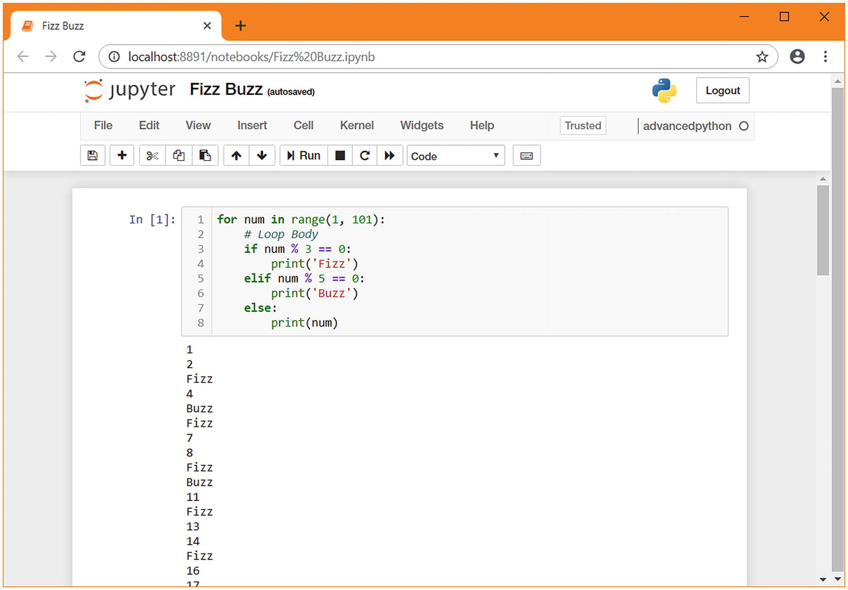
fizzbuzz in a Jupyter notebook
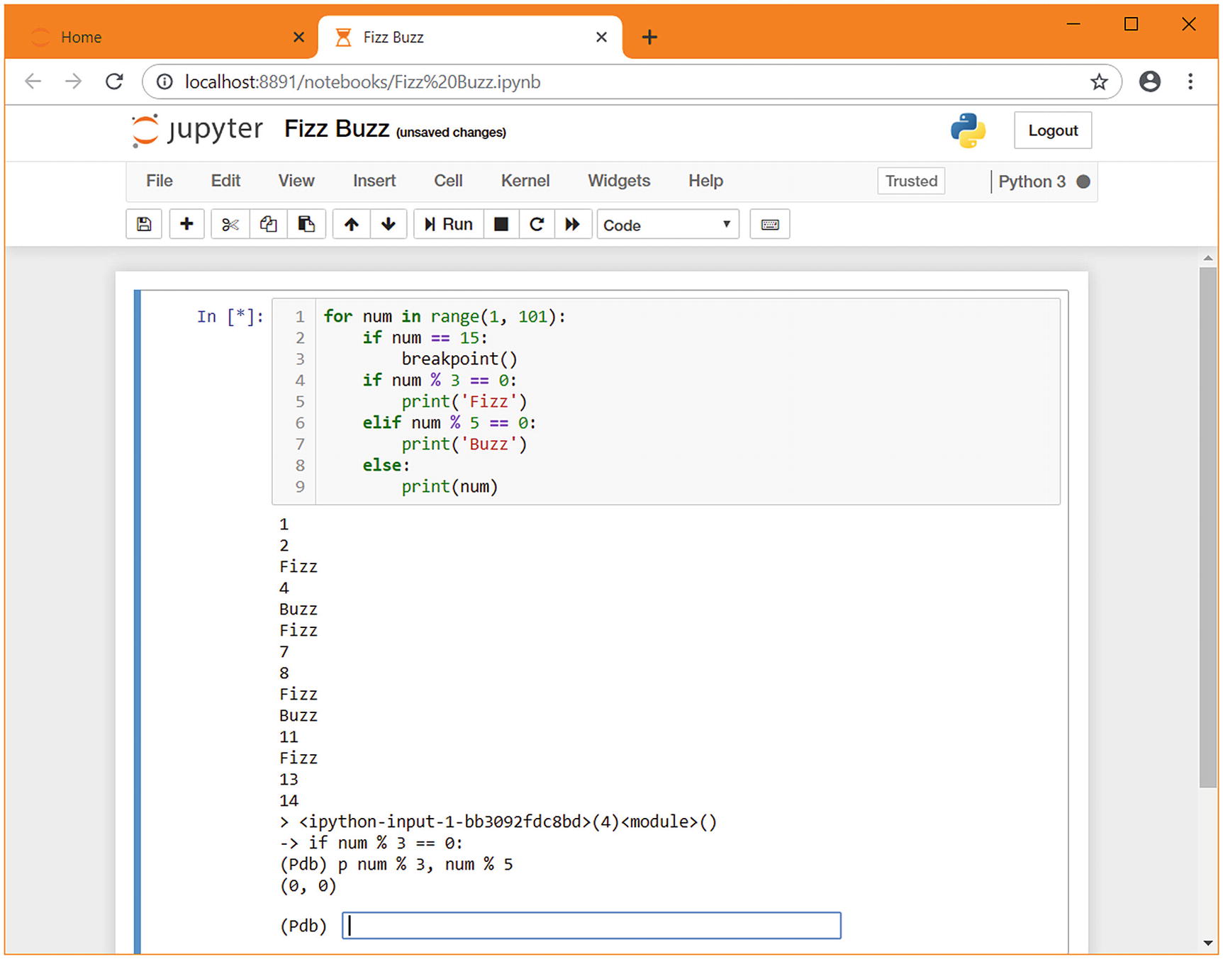
pdb in a Jupyter notebook
Prototyping in this chapter
There are advantages and disadvantages to all the methods we’ve explored, but each has its place. For very simple one-liners, such as list comprehensions, I often use the REPL, as it’s the fastest to start up and has no complex control flow that would be hard to debug.
For more complex tasks, such as bringing functions from external libraries together and doing multiple things with them, a more featureful approach is usually more efficient. I encourage you to try different approaches when prototyping things to understand where the sweet spot is in terms of convenience and your personal preferences.
Comparison of prototyping environments
Feature | REPL | Script | Script + pdb | Jupyter | Jupyter + pdb |
|---|---|---|---|---|---|
Indenting code | Strict rules | Normal rules | Normal rules | Normal rules | Normal rules |
Re-running previous commands | Single typed line | Entire script only | Entire script or jump to the previous line | Logical blocks | Logical blocks |
Stepping | Indented blocks run as one | The entire script runs as one | Step through statements | Logical blocks run as one | Step through statements |
Introspection | Can introspect between logical blocks | No introspection | Can introspect between statements | Can introspect between logical blocks | Can introspect between statements |
Persistence | Nothing is saved | Commands are saved | Commands are saved, interactions at the pdb prompt are not | Commands and output are saved | Commands and output are saved |
Editing | Commands must be reentered | Any command can be edited, but the whole script must be re-run | Any command can be edited, but the whole script must be re-run | Any command can be edited, but the logical block must be re-run | Any command can be edited, but the logical block must be re-run |
In this chapter, we will be prototyping a few different functions that return data about the system they’re running on. They will depend on some external libraries, and we may need to use some simple loops, but not extensively.
As we’re unlikely to have complex control structures, the indenting code feature isn’t a concern. Re-running previous commands will be useful as we’re dealing with multiple different data sources. It’s possible that some of these data sources will be slow, so we don’t want to be forced to always re-run every data source command when working on one of them. That discounts the REPL and is a closer fit for Jupyter than the script-based processes.
We want to be able to introspect the results of each data source, but we are unlikely to need to introspect the internal variables of individual data sources, which suggests the pdb-based approaches are not necessary (and, if that changes, we can always add in a breakpoint() call). We will want to store the code we’re writing, but that only discounts the REPL which has already been discounted. Finally, we want to be able to edit code and see the difference it makes.
If we compare these requirements to Table 1-1, we can create Table 1-2, which shows that the Jupyter approach covers all of the features we need well, whereas the script approach is good enough but not quite optimal in terms of ability to re-run previous commands.
Matrix of whether the features of the various approaches match our requirements9
Feature | REPL | Script | Script + pdb | Jupyter | Jupyter + pdb |
|---|---|---|---|---|---|
Indenting code | ✔ | ✔ | ✔ | ✔ | ✔ |
Re-running previous commands | ❌ | ⚠ | ⚠ | ✔ | ✔ |
Stepping | ❌ | ❌ | ⚠ | ✔ | ⚠ |
Introspection | ✔ | ✔ | ✔ | ✔ | ✔ |
Persistence | ❌ | ✔ | ✔ | ✔ | ✔ |
Editing | ❌ | ✔ | ✔ | ✔ | ✔ |
Environment setup
There has been a long history of systems to create isolated environments in Python. The one you’ll most likely have used before is called virtualenv . You may also have used venv, conda, buildout, virtualenvwrapper, or pyenv. You may even have created your own by manipulating sys.path or creating lnk files in Python’s internal directories.
Each of these methods has positives and negatives (except for the manual method, for which I can think of only negatives), but pipenv has excellent support for managing direct dependencies while keeping track of a full set of dependency versions that are known to work correctly and ensuring that your environment is kept up to date. That makes it a good fit for modern pure Python projects. If you’ve got a workflow that involves building binaries or working with outdated packages, then sticking with the existing workflow may be a better fit for you than migrating it to pipenv. In particular, if you’re using Anaconda because you do scientific computing, there’s no need to switch to pipenv. If you wish, you can use pipenv --site-packages to make pipenv include the packages that are managed through conda as well as its own.
Pipenv’s development cycle is rather long, as compared to other Python tools. It’s not uncommon for it to go months or years without a release. In general, I’ve found pipenv to be stable and reliable, which is why I’m recommending it. Package managers that have more frequent releases sometimes outstay their welcome, forcing you to respond to breaking changes regularly.
For pipenv to work effectively, it does require that the maintainers of packages you’re declaring a dependency on correctly declare their dependencies. Some packages do not do this well, for example, by specifying only a dependency package without any version restrictions when restrictions exist. This problem can happen, for example, because a new major release of a subdependency has recently been released. In these cases, you can add your own restrictions on what versions you’ll accept (called a version pin).
If you find yourself in a situation where a package is missing a required version pin, please consider contacting the package maintainers to alert them. Open source maintainers are often very busy and may not yet have noticed the issue – don’t assume that just because they’re experienced that they don’t need your help. Most Python packages have repositories on GitHub with an issue tracker. You see from the issue tracker if anyone else has reported the problem yet, and if not, it is an easy way to contribute to the packages that are easing your development tasks.
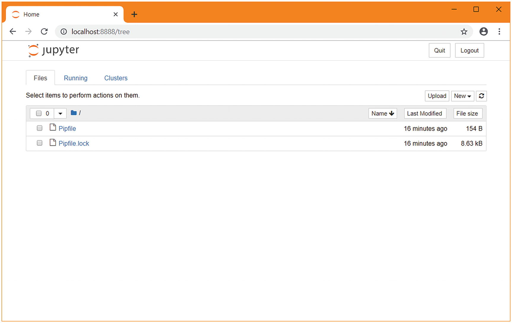
Setting up a new project
The final line here instructs the copy of IPython within the isolated environment to install itself as an available kernel for the current user account, with the name advancedpython. This allows us to select the kernel without having to activate this isolated environment manually each time. Installed kernels can be listed with jupyter kernelspec list and removed with jupyter kernelspec remove.
A web browser automatically opens and displays the Jupyter interface with a directory listing of the directory we created. This will look like Figure 1-3. With the project set up, it’s time to start prototyping. Choose “New” and then “advancedpython”.
The Jupyter home screen in a new pipenv directory
Prototyping our scripts
A logical first step is to create a Python program that returns various information about the system it is running on. Later on, these pieces of information will be part of the data that’s aggregated, but for now some simple data is an appropriate first objective.
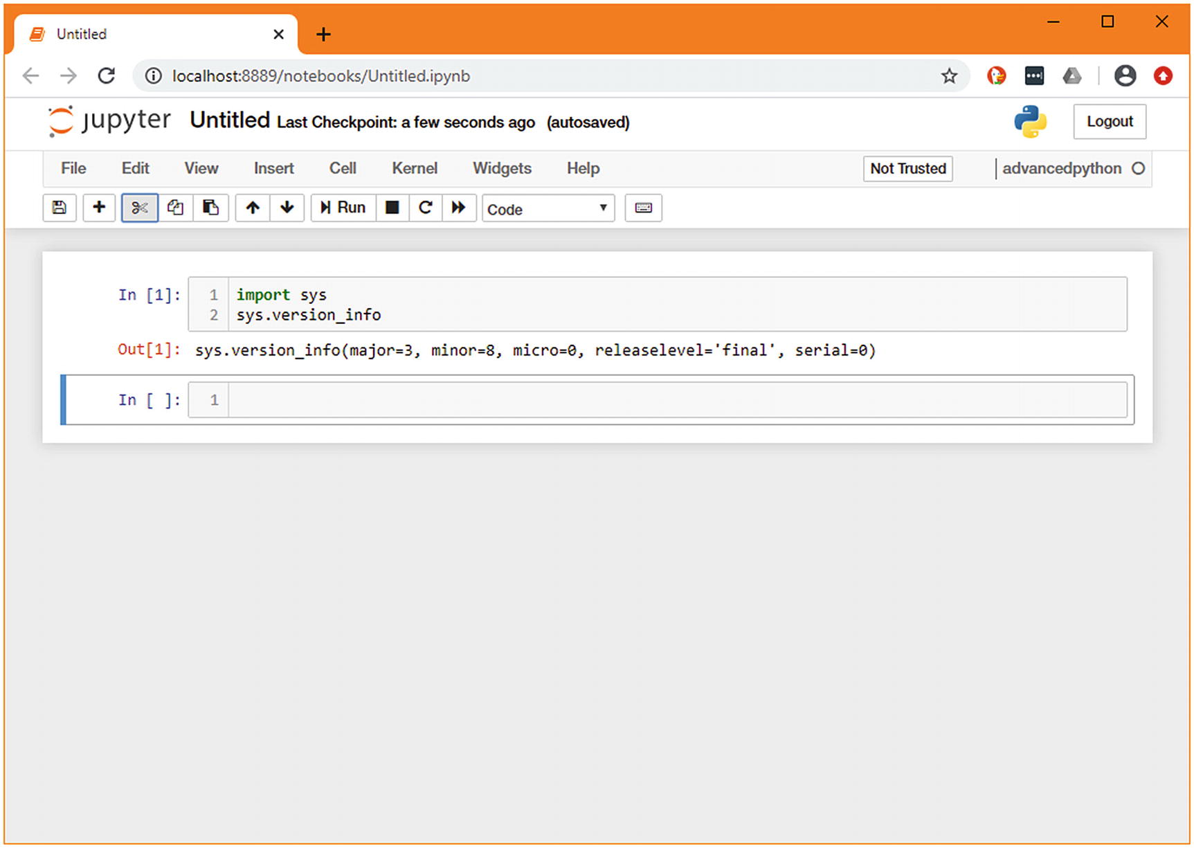
A simple Jupyter notebook showing sys.version_info
Jupyter shows the value of the last line of the cell, as well as anything explicitly printed. As the last line of our cell is sys.version_info, that is what is shown in the output.10
Another useful piece of information to aggregate is the current machine’s IP address. This isn’t exposed in a single variable; it’s the result of a few API calls and processing of information. As this requires more than a simple import, it makes sense to build up the variables step by step in new cells. When doing so, you can see at a glance what you got from the previous call, and you have those variables available in the next cell. This step-by-step process allows you to concentrate on the new parts of the code you’re writing, ignoring the parts you’ve completed.
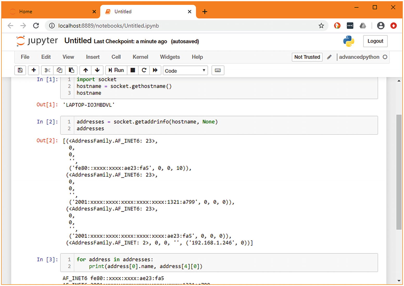
Prototyping a complex function in multiple cells11

The result of merging the cells from Figure 1-5
Installing dependencies
A more useful thing to know would be how much load the system is experiencing. In Linux, this can be found by reading the values stored in /proc/loadavg. In macOS this is sysctl -n vm.loadavg. Both systems also include it in the output of other programs, such as uptime, but this is such a common task that there is undoubtedly a library that can help us. We don’t want to add any complexity if we can avoid it.
We have no preferences about which version of psutil is needed, so we have not specified a version. The install command adds the dependency to Pipfile and the particular version that is picked to Pipfile.lock . Files with the extension .lock are often added to the ignore set in version control. You should make an exception for Pipfile.lock as it helps when reconstructing old environments and performing repeatable deployments.
When we return to the notebook, we need to restart the kernel to ensure the new dependency is available. Click the Kernel menu, then restart. If you prefer keyboard shortcuts , you can press <ESCAPE> to exit editing mode (the green highlight for your current cell will turn blue to confirm) and press 0 (zero) twice.
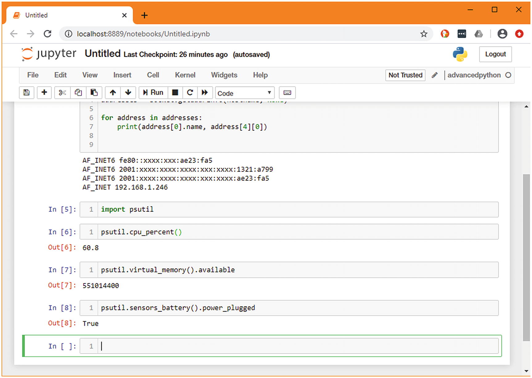
and click Run (or, <SHIFT+ENTER> to run the cell from the keyboard). In a new cell, type psutil.cpu<TAB>.12 You’ll see the members of psutil that jupyter can autocomplete for you. In this case, cpu_stats appears to be a good option, so type that out. At this point, you can press <SHIFT+TAB> to see minimal documentation on cpu_stats, which tells us that it doesn’t require any arguments.
Numerous other functions in the psutil library make good sources of data, so let’s create a cell for each function that looks interesting. There are different functions available on different operating systems, so be aware that if you’re following this tutorial on Windows, you have a slightly more limited choice of functions.
Try the autocomplete and help functions of Jupyter to get a feel for what information you find useful and create at least one more cell that returns data.
Including psutil’s import in each cell would be repetitive and not good practice for a Python file, but we do want to make sure it’s easy to run a single function in isolation. To solve this, we’ll move the imports to a new top cell, which is the equivalent of the module scope in a standard Python file.
An example of a complete notebook following the exercise
While you’ve been doing this, the numbers in square brackets next to the cell have been increasing. This number is the sequence of operations that have been run. The number next to the first cell has stayed constant, meaning this cell hasn’t been run while we’ve experimented with the lower one.
In the Cell menu, there is an option to Run All, which will run each cell in sequence like a standard Python file. While it’s useful to be able to run all cells to test the entire notebook, being able to run each cell individually lets you split out complex and slow logic from what you’re working on without having to re-run it each time.
Exporting to a .py file
Although Jupyter has served us well as a prototyping tool, it’s not a good match for the main body of our project. We want a traditional Python application, and the great presentation features of Jupyter aren’t useful right now. Jupyter has built-in support for exporting notebooks in a variety of formats, from slideshows to HTML, but the one we’re interested in is Python scripts.
Untitled.py, generated from the preceding notebook
As you can see, each cell is separated from the others with comments, and the standard boilerplate around text encoding and shebang is present at the top of the file. Starting the prototyping in Jupyter rather than directly in a Python script or in the REPR hasn’t cost us anything in terms of flexibility or time; rather it gave us more control over how we executed the individual blocks of code while we were exploring.
serverstatus.py
Building a command-line interface
These functions alone are not especially useful, most only each wrap an existing Python function. The obvious thing we want to do is to print their data, so you may wonder why we’ve gone to the trouble of creating single-line wrapper functions. This will be more obvious as we create more complex data sources and multiple ways of consuming them, as we will benefit from not having special-cased the simplest ones. For now, to make these useful, we can give users a simple command-line application that displays this data.
However, if you load code through an interactive session or by providing a path to a script to run, then it can’t necessarily be imported. Such modules, therefore, get the special name "__main__". The ifmain trick is used to detect if that is the case. That is, if the module has been specified on the command line as the file to run, then the contents of the block will execute. The code inside this block will not execute when the module is imported by other code because the __name__ variable would be set to the name of the module instead. Without this guard in place, the command-line handler would execute whenever this module is imported, making it take over any program that uses these utility functions.
As the contents of the ifmain block can only be run if the module is the entrypoint into the application, you should be careful to keep it as short as possible. Generally, it’s a good idea to limit it to a single statement that calls a utility function. This allows that function call to be testable and is required for some of the techniques we will be looking at in the next chapter.
The sys module and argv
Most programming languages expose a variable named argv, which represents the name of the program and the arguments that the user passed on invocation. In Python, this is a list of strings where the first entry is the name of the Python script (but not the location of the Python interpreter) and any arguments listed after that.
Without checking the argv variable, we can only produce very basic scripts. Users expect a command-line flag that provides help information about the tool. Also, all but the simplest of programs need to allow users to pass configuration variables in from the command line.
sensors_argv.py – cli using manual checking of argv
The command_line(...) function is not overly complicated, but this is a very simple program. You can easily imagine situations where there are multiple flags allowed in any order and configurable variables being significantly more complex. This is only practically possible because there is no ordering or parsing of values involved. Some helper functionality is available in the standard library to make it easier to create more involved command-line utilities.
argparse
The argparse module is the standard method for parsing command-line arguments without depending on external libraries. It makes handling the complex situations alluded to earlier significantly less complicated; however, as with many libraries that offer developers choices, its interface is rather difficult to remember. Unless you’re writing command-line utilities regularly, it’s likely to be something that you read the documentation of every time you need to use it.
The model that argparse follows is that the programmer creates an explicit parser by instantiating argparse.ArgumentParser with some basic information about the program, then calling functions on that parser to add new options. Those functions specify what the option is called, what the help text is, any default values, as well as how the parser should handle it. For example, some arguments are simple flags, like --dry-run; others are additive, like -v, -vv, and -vvv; and yet others take an explicit value, like --config config.ini.
We aren’t using any parameters in our program just yet, so we skip over adding these options and have the parser parse the arguments from sys.argv . The result of that function call is the information it has gleaned from the user. Some basic handling is also done at this stage, such as handling --help, which displays an autogenerated help screen based on the options that were added.
sensors_argparse.py – cli using the standard library module argparse
click
Click is an add-on module that simplifies the process of creating command-line interfaces on the assumption that your interface is broadly similar to the standard that people expect. It makes for a significantly more natural flow when creating command-line interfaces and encourages you toward intuitive interfaces.
Whereas argparse requires the programmer to specify the options that are available when constructing a parser, click uses decorators on methods to infer what the parameters should be. This approach is a little less flexible, but easily handles 80% of typical use cases. If you’re writing a command-line interface, you generally want to follow the lead of other tools, so it is intuitive for the end-user.
sensors_click.py – cli using the contributed library click
Extract from sensors_click_bold.py
Click also provides transparent support for autocomplete in terminals and a number of other useful functions. We will revisit these later in the book when we expand on this interface.
Pushing the boundaries
We’ve looked at using Jupyter and IPython for doing prototyping, but sometimes we need to run prototype code on a specific computer, rather than the one we’re using for day-to-day development work. This could be because the computer has a peripheral or some software we need, for example.
This is mainly a matter of comfort; editing and running code on a remote machine can vary from slightly inconvenient to outright difficult, especially when there are differences in the operating system.
In the preceding examples, we’ve run all the code locally. However, we are planning to run the final code on a Raspberry Pi as that’s where we attach our specialized sensors. As an embedded system, it has significant hardware differences, both in terms of performance and peripherals.
Remote kernels
Testing this code would require running a Jupyter environment on a Raspberry Pi and connecting to that over HTTP or else connecting over SSH and interacting with the Python interpreter manually. This is suboptimal, as it requires ensuring that the Raspberry Pi has open ports for Jupyter to bind to and requires manually synchronizing the contents of notebooks between the local and remote hosts using a tool like scp. This is even more of a problem with real-world examples. It’s hard to imagine opening a port on a server and connecting to Jupyter there to test log analysis code.
Instead, it is possible to use the pluggable kernel infrastructure of Jupyter and IPython to connect a locally running Jupyter notebook to one of many remote computers. This allows testing of the same code transparently on multiple machines and with minimal manual work.
When Jupyter displays its list of potential execution targets, it is listing its list of known kernel specifications. When a kernel specification has been selected, an instance of that kernel is created and linked to the notebook. It is possible to connect to remote machines and manually start an individual kernel for your local Jupyter instance to connect to. However, this is rarely an effective use of time. When we ran pipenv run ipython kernel install at the start of this chapter, we were creating a new kernel specification for the current environment and installing that into the list of known kernel specifications.
Some low-performance hosts, such as Raspberry Pis, may make installing ipython_kernel frustratingly slow. In this case, you may consider using the package manager’s version of ipython_kernel instead. The ipython kernel does require many support libraries which may take some time to install on a low-powered computer. In that case, you could set up the environment as
You would then install the ipython_kernel package as normal using pipenv install. If you’re using a Raspberry Pi running Raspbian, you should always add piwheels to your Pipfile, as Raspbian comes preconfigured to use PiWheels globally. Not listing it in your Pipfile can cause installations to fail.
This output shows us how Jupyter would run the kernel if it were installed on that computer. We can use the information from this specification to create a new remote_ikernel specification on our development machine that points at the same environment as the development-testing kernel on the Raspberry Pi.
The --kernel_cmd parameter is the contents of the argv section from the kernel spec file. Each line is space separated and without the individual quotation marks. This is the command that starts the kernel itself.
The --name parameter is the equivalent of display_name from the original kernel spec. This is what will be shown in Jupyter when you select this kernel, alongside SSH information. It doesn’t have to match the remote kernel’s name that you’ve copied from, it’s just for your reference.
The --interface and --host parameters define how to connect to the remote machine. You should ensure that passwordless15 SSH is possible to this machine so that Jupyter can set up connections.
The --workdir parameter is the default working directory that the environment should use. I recommend setting this to be the directory that contains your remote Pipfile.
The --language parameter is the value of the language value from the original kernel spec to differentiate different programming languages.
If you’re having difficulty connecting to the remote kernel, you can try opening a shell using Jupyter on the command line. This often shows useful error messages. Find the name of the kernel using jupyter kernelspec list and then use that with jupyter console:
At this point, when we reenter the Jupyter environment, we see a new kernel available that matches the connection information we supplied. We can then select that kernel and execute commands that require that environment,16 with the Jupyter kernel system taking care of connecting to the Raspberry Pi and activating the environment in ~/development-testing.
Developing code that cannot be run locally
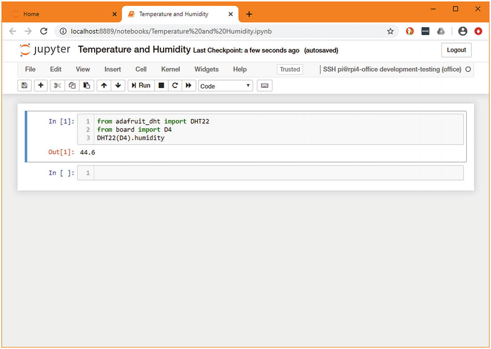
There are some useful sensors available on the Raspberry Pi; these provide the actual data that we are interested in collecting. In other use cases, this might be information gathered by calling custom command-line utilities, introspecting a database, or making local API calls.
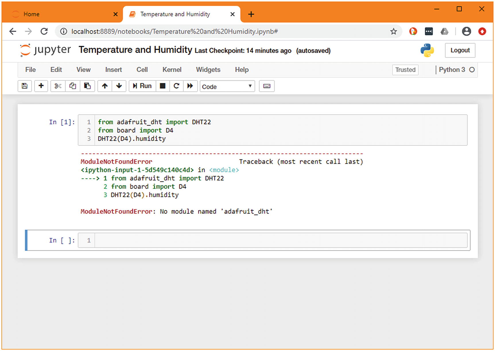
This isn’t a book on how to make the most of the Raspberry Pi, so we will gloss over much of the detail of exactly how it does its work, but suffice it to say that there is a large amount of documentation and support for doing exciting things using Python. In this case, there is a library that we want to use that provides a function to retrieve both temperature and relative humidity from a sensor that can be added to the board. Like many other tasks, this is relatively slow (it can take a good portion of a second to measure) and requires a specific environment (an external sensor being installed) to execute. In that way, it is similar to monitoring active processes on a web server by communicating through their management ports.
This results in the Pipfile and Pipfile.lock files being updated to include this dependency. We want to make use of these dependencies on the remote host, so we must copy these files across and install them using Pipenv. It would be possible to run this command in both environments, but that risks mistakes creeping in. Pipenv assumes that you use the same version of Python for both development and deployment, in keeping with its philosophy of avoiding problems during deployment. For that reason, if you’re planning to deploy to a set version of Python, you should use that for development locally.
However, if you do not want to install unusual versions of Python in your local environment, or if you’re targeting multiple different machines, it is possible to deactivate this check. To do so, remove the python_version line from the end of your Pipfile. This allows your environment to be deployed to any Python version. However, you should ensure that you’re aware of what versions you need to support and test accordingly.
Be aware, however, that if you’ve created your Pipfile on a different operating system or a different CPU architecture (such as files created on a standard laptop and installed on a Raspberry Pi), it is possible that the pinned packages will not be suitable when deploying them on another machine. In this case, it is possible to relock the dependencies without triggering version upgrades by running pipenv lock --keep-outdated.
You now have the specified dependencies available in the remote environment. If you’ve relocked the files, you should transfer the changed lock file back and store it, so you can redeploy in future without having to regenerate this file. At this stage, you can connect to the remote server through your Jupyter client and begin prototyping. We’re looking to add the humidity sensor, so we’ll use the library we just added and can now receive a valid humidity percentage.
Jupyter connected to a remote Raspberry Pi
Demonstration of the same code being run on the local machine
This allows for the function to be called on any machine, unless it has a temperature and humidity sensor connected to pin D4 and to return a None anywhere else.
The completed script
The final version of our script from this chapter
Summary
This concludes the chapter on prototyping; in the following chapters, we will build on the data extraction functions we’ve created here to create libraries and tools that follow Python best practice. We have followed the path from playing around with a library up to the point of having a working shell script that has genuine utility. As we continue, it will develop to better fit our end goal of distributed data aggregation.
The tips we’ve covered here can be useful at many points in the software development life cycle, but it’s important not to be inflexible and only follow a process. While these methods are effective, sometimes opening the REPL or using pdb (or even plain print(...) calls) will be more straightforward than setting up a remote kernel. It is not possible to pick the best way of approaching a problem unless you’re aware of the options.
- 1.
Jupyter is an excellent tool for exploring libraries and doing initial prototyping of their use.
- 2.
There are special-purpose debuggers available for Python that can be integrated easily into your workflow using the breakpoint() function and environment variables.
- 3.
Pipenv helps you to define version requirements that are kept up to date, involve minimal specification, and facilitate reproducible builds.
- 4.
The library click allows for simple command-line interfaces in an idiomatic Python style.
- 5.
Jupyter’s kernel system allows for seamless integration of multiple programming languages running both locally and on other computers into a single development flow.
Additional resources
The Pipenv documentation at https://pipenv.pypa.io/en/latest/ has a lot of useful explanation on customizing pipenv to work as you want, specifically with regard to customizing virtual environment creation and integration into existing processes. If you’re new to pipenv but have used virtual environments a lot, then this has good documentation to help you bridge the gap.
If you’re interested in prototyping other programming languages in Jupyter, I’d recommend you read through the Jupyter documentation at https://jupyter.readthedocs.io/en/latest/ – especially the kernels section.
For information on Raspberry Pis and compatible sensors, I recommend the CircuitPython project’s documentation on the Raspberry Pi: https://learn.adafruit.com/circuitpython-on-raspberrypi-linux.