
2
ELECTROMAGNETIC FUNDAMENTALS FOR SIGNAL INTEGRITY
2.1 Maxwell’s Equations
2.2 Common Vector Operators
2.2.1 Vector
2.2.2 Dot Product
2.2.3 Cross Product
2.2.4 Vector and Scalar Fields
2.2.5 Flux
2.2.6 Gradient
2.2.7 Divergence
2.2.8 Curl
2.3 Wave Propagation
2.3.1 Wave Equation
2.3.2 Relation Between E and H and the Transverse Electromagnetic Mode
2.3.3 Time-Harmonic Fields
2.3.4 Propagation of Time-Harmonic Plane Waves
2.4 Electrostatics
2.4.1 Electrostatic Scalar Potential in Terms of an Electric Field
2.4.2 Energy in an Electric Field
2.4.3 Capacitance
2.4.4 Energy Stored in a Capacitor
2.5 Magnetostatics
2.5.1 Magnetic Vector Potential
2.5.2 Inductance
2.5.3 Energy in a Magnetic Field
2.6 Power Flow and the Poynting Vector
2.6.1 Time-Averaged Values
2.7 Reflections of Electromagnetic Waves
2.7.1 Plane Wave Incident on a Perfect Conductor
2.7.2 Plane Wave Incident on a Lossless Dielectric
References
Problems
Much of signal integrity is based heavily in electromagnetic theory. Various aspects of this theory are found in numerous books on a variety of topics, such as microwaves, electromagnetics, optics, and mathematics. To rely on these books to form a basis of the fundamental understanding of signal integrity would result in a confusing disarray of conflicting assumptions, notations, and conventions. Although it is assumed that readers have a basic understanding of electromagnetics, the presentation of Maxwell’s equations and subsequent solutions in the form most often used in signal integrity will minimize confusion and help readers extract the relevance from the haze of mathematical calculation often encountered in generalized electromagnetic textbooks. It is also convenient to summarize, in one place, the underlying physics that forms the basis of succeeding chapters. In this section we present Maxwell’s equations and the underlying electromagnetic theory needed for signal integrity. The concepts are used and expanded on in several subsequent chapters. This analysis does not constitute a complete theo-retical study; however, it does present the fundamental electromagnetic concepts needed to develop the basis of signal integrity theory. As the book progresses, this material will be built on to describe more advanced concepts as they are applied to real-world examples.
Initially, the most common vector operators are reviewed briefly. This is important because Maxwell’s equations will be presented in differential form and a fundamental understanding of the vector operators will allow readers to visualize the behavior of electromagnetic fields. Next, the equations that govern a plane wave propagating in free space are derived directly from Maxwell’s equations. Then the concepts of wave propagation, intrinsic impedance, and the speed of light are derived. Next, the theory of electrostatics and magnetostatics is covered to explain the physical meaning of an electric and a magnetic field, the energy they contain, and how they relate to specific circuit elements, such as inductance and capacitance, used in later chapters. Finally, we discuss the power carried by electromagnetic waves and how they react when propagating into different materials, such as metal or other dielectric regions. Other aspects of electromagnetic theory are covered in later chapters, but the basis of that analysis is defined here.
2.1 MAXWELL’S EQUATIONS
Electromagnetic theory is described by Maxwell’s equations, published originally in 1873. In this section we outline the fundamentals of electromagnetic theory that we will need for the remainder of the book. Since a broad study of Maxwell’s equations is beyond our scope in this text, we present only the necessary information that applies directly to the specific problems addressed here. Note that it is assumed that readers have completed basic electromagnetic theory classes as a prerequisite to this material.
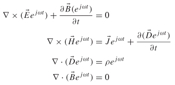
The differential form of Maxwell’s equations in SI units is summarized in equations (2-1) through (2-4). The equivalent integral forms of Maxwell’s equations are presented throughout when necessary; however, emphasis is placed on the differential forms when convenient because they lend themselves to better intuitive understanding:
Electromagnetic fields are derived from the movement of charge, so ![]() and ρ are the ultimate sources that induce the electric and magnetic fields, while the other quantities are responses. Note that the magnetization density,
and ρ are the ultimate sources that induce the electric and magnetic fields, while the other quantities are responses. Note that the magnetization density, ![]() , does not exist in nature, as it is a mere mathematical convenience. Realistic sources of magnetic current are caused by an electric current loop, as opposed to the flow of a magnetic charge, which is discussed in detail in Section 2.5. The magnetization density is included here only for completeness, as it is typically not used for the applications covered in this book. The constants μ0 and ε0 dictate the electromagnetic properties of free space, such as the speed of light and the intrinsic impedance, both of which are discussed in more detail in Section 2.3.
, does not exist in nature, as it is a mere mathematical convenience. Realistic sources of magnetic current are caused by an electric current loop, as opposed to the flow of a magnetic charge, which is discussed in detail in Section 2.5. The magnetization density is included here only for completeness, as it is typically not used for the applications covered in this book. The constants μ0 and ε0 dictate the electromagnetic properties of free space, such as the speed of light and the intrinsic impedance, both of which are discussed in more detail in Section 2.3.
Equations (2-1) through (2-6) are not sufficient to describe the electromagnetic properties of general materials; they must be supplemented with relations that comprehend the properties of media other than free space. Specifically, equation (2-7) comprehends the finite conductivity of metal, equation (2-8) accounts for the magnetic properties of a material, and equation (2-9) describes how the dielectric will respond to an applied electric field:
where ![]() is the current density (A/m2), σ the conductivity of a medium (e.g., a metal) (S/m), μr the relative permeability, and εr the relative permittivity (also known as the relative dielectric constant). Note that both μr and εr are unitless quantities. The convention used in this book is to represent the equivalent relative permittivity and permeability as
is the current density (A/m2), σ the conductivity of a medium (e.g., a metal) (S/m), μr the relative permeability, and εr the relative permittivity (also known as the relative dielectric constant). Note that both μr and εr are unitless quantities. The convention used in this book is to represent the equivalent relative permittivity and permeability as
For use in high-speed digital design, materials included typically have descriptive coefficients σ, μr, and εr that are linear, meaning that they do not change as a function of the applied field. However, for many realistic dielectric materials used to construct circuit boards in digital designs, the descriptive coefficients are not homogeneous (independent of position) or isotropic (independent of direction), meaning that extreme care must be taken to ensure that the material properties are accounted for properly, which is explored in detail in Chapter 6. Furthermore, the descriptive coefficients often exhibit strong frequency dependence, the nature of which is explored throughout the book.
Although this brief review of Maxwell’s equations may initially seem intimidating, throughout the book the theory will be simplified and applied directly to the solution of practical real-world problems, allowing readers to extract the important concepts from the haze of mathematical calculations so that an intuitive understanding can be conveyed.
2.2 COMMON VECTOR OPERATORS
Maxwell’s equations are presented in differential form using many vector operators, which simplifies their representation. The vector operators describe the behavior of the fields and how they interact, so a full understanding of the meaning behind these operators will allow readers to visualize the problem, which will lead to an intuitive understanding. In engineering, the most valuable tool is a comprehensive understanding of the concept. In electromagnetics and signal integrity, the concept is often best understood through visualization of the fields. The vector operators used in this book are reviewed here, with an emphasis on how they affect the fields visually.
2.2.1 Vector
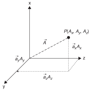
In physics and in vector calculus, a vector is a concept characterized by a mag-nitude and a direction. A component of a vector is the influence of that vector in a given direction. A vector is often described by a fixed number of components that sum uniquely to the total vector. When used in this role, the choice of directions is dependent on the particular coordinate system being used: Cartesian coordinates, spherical coordinates, or polar coordinates. A common example of a vector is force, because it has a magnitude and a direction. Whenever possible, the problems and analysis are presented in rectangular (Cartesian) coordinates. When the geometry of the problem dictates coordinate transformation into a spherical or cylindrical coordinate system, the relevant transformations are given in Appendix A.
Recall that if the vector ![]() was located at the point in space P(x,y,z), with the components
was located at the point in space P(x,y,z), with the components ![]() xA1,
xA1, ![]() yA2, and
yA2, and ![]() zA3, where
zA3, where ![]() m is a unit vector along the axis m, the expression for
m is a unit vector along the axis m, the expression for ![]() could be written
could be written
where the magnitude of the vector is shown as
This vector is shown graphically in Figure 2-1.
2.2.2 Dot Product
The dot product of two vectors ![]() and
and ![]() is a metric of how much parallelism exists between vectors:
is a metric of how much parallelism exists between vectors:
where ϕ is the angle between ![]() and
and ![]() . Note that if ϕ is 90°, then
. Note that if ϕ is 90°, then ![]() ·
· ![]() = 0, and if ϕ is 0° (the vectors are parallel), then
= 0, and if ϕ is 0° (the vectors are parallel), then ![]() ·
· ![]() = AB, which is simply the product of their magnitudes.
= AB, which is simply the product of their magnitudes.
Figure 2-1 Graphical representation of a vector in rectangular coordinates.
If the vectors ![]() and
and ![]() are expressed in terms of their generalized orthogonal components as in (2-11) and the expression is expanded, the dot product can be calculated as
are expressed in terms of their generalized orthogonal components as in (2-11) and the expression is expanded, the dot product can be calculated as
2.2.3 Cross Product
Similarly, the cross product of ![]() and
and ![]() is a measure of how orthogonal the vectors are, as shown by
is a measure of how orthogonal the vectors are, as shown by
where ![]() n is a unit vector normal to the plane containing
n is a unit vector normal to the plane containing ![]() and
and ![]() .If ϕ is 0°, then
.If ϕ is 0°, then ![]() ×
× ![]() = 0, and if ϕ is 90° (the vectors are at a right angle to each other), then
= 0, and if ϕ is 90° (the vectors are at a right angle to each other), then ![]() ×
× ![]() = AB
= AB ![]() n with a direction perpendicular to both
n with a direction perpendicular to both ![]() and
and ![]() , with the ambiguity of direction resolved by means of the right-hand rule, as shown in Figure 2-2. If the angle between
, with the ambiguity of direction resolved by means of the right-hand rule, as shown in Figure 2-2. If the angle between ![]() and
and ![]() is something other than 0° or 90°, the following determinant form of the cross product applies:
is something other than 0° or 90°, the following determinant form of the cross product applies:
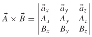
which simplifies to
Figure 2-2 Graphical representation of the cross product.
2.2.4 Vector and Scalar Fields
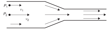
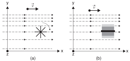
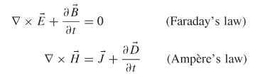
In electromagnetic theory, a field is defined as a mathematical function of space and time. Fields can be classified as either scalar or vector. A scalar field has a specific value (magnitude) at every point in a region of space at each instance in time. Figure 2-3 shows two examples of a scalar field, temperature in a block of material and the voltage across a resistive strip. Note that each point P(x, y, z), there exists a corresponding temperature T(x, y, z) or voltage v(x) at any instant in time. Other examples of scalar fields are pressure and density. A vector field has a variable magnitude and direction at any point in time, as illustrated with Figure 2-4. Note that the velocity and direction of the fluid inside the pipe changes in the vicinity of the neck-down region, so the magnitude and direction (phase) of the vectors that describe the motion of the fluid at a given instant in time are a function of the position in space. Other examples of vector fields are acceleration and electric and magnetic fields.
2.2.5 Flux
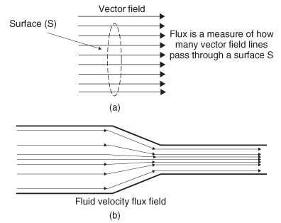
A vector field, ![]() (x, y, z, t), can be represented graphically by depicting a large number of individual vectors with a specific magnitude and phase (direction); however, this is cumbersome. A more useful method for representation of a vector field is to use the concept of flux. Flux is a measure of how many field vectors pass though a surface in space, as depicted in Figure 2-5a. The net flux of vector field
(x, y, z, t), can be represented graphically by depicting a large number of individual vectors with a specific magnitude and phase (direction); however, this is cumbersome. A more useful method for representation of a vector field is to use the concept of flux. Flux is a measure of how many field vectors pass though a surface in space, as depicted in Figure 2-5a. The net flux of vector field ![]() through surface S is shown as
through surface S is shown as
Figure 2-3 Examples of scalar fields: (a) temperature; (b) voltage.
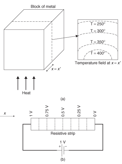
Figure 2-4 Example of a vector field: fluid velocity.
A flux plot can replace vectors with a system of flux lines that are created in accordance with the following rules:
1. The transverse density of the flux lines agrees with the magnitudes of the vectors. So, in Figure 2-5b, the velocity of the fluid is slower near the pipe wall, necessitating that the flux lines be drawn farther apart than in the middle, where the fluid flow is faster.
2. The direction of the flux lines must agree with the direction of the vectors.
Figure 2-5 (a) Definition of flux; (b) example of a flux field.
Flux is, however, useful for more than just simplifying a vector field. If a surface S is drawn in a region of space that includes flux lines, the number of flux lines passing through that surface is a measure of several physical quantities, such as current or power flow. Note that if (2-17) is integrated over a closed surface, the net flux will always be zero, assuming that no sources exist within the volume of the closed surface. This is because the same number of flux lines enter the volume as exit it.
To illustrate the utility of the flux concept with an example, consider current flow in a wire. Suppose that a wire contains electric charges of density ρ(C/m3) in a region and the charges have a velocity v(m/s). The current density in the region is calculated as
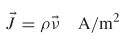
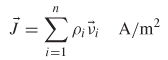
the instantaneous rate of charge flow per unit cross-sectional area at point P in space. For n points in space with charge densities ρi and velocities vi, the current density becomes
Therefore, the total current flowing through a surface (e.g., the cross section of the wire) is the sum of all the current density functions within the area of the surface times the surface area. This calculates the total number of vectors (![]() ) passing though the cross-sectional surface S of the wire, which is flux. Therefore, the flux of the current density function is the current flowing through area S and is calculated as
) passing though the cross-sectional surface S of the wire, which is flux. Therefore, the flux of the current density function is the current flowing through area S and is calculated as

Figure 2-6 Current flux through a wire.
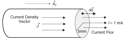
Example 2-1 If a current of 1 mA is measured flowing through a wire with a radius of 5 mm, calculate the current density. See Figure 2-6.
SOLUTION Assume that the current density is constant in the cross section so that ![]() =
= ![]() z J = J z and A is the cross-sectional area of the wire.
z J = J z and A is the cross-sectional area of the wire.
Therefore,
![]()
2.2.6 Gradient
The vector operator ![]() , pronounced del, is shorthand for the gradient of a scalar field. In simple terms, the gradient is the space rate of change of a scalar field. In rectangular coordinates, the gradient of a function f is
, pronounced del, is shorthand for the gradient of a scalar field. In simple terms, the gradient is the space rate of change of a scalar field. In rectangular coordinates, the gradient of a function f is
Subsequently, the gradient constructs a vector field from a scalar field.
2.2.7 Divergence
The divergence of a vector field ![]() is a measure of the outward flux per unit volume. For example, if
is a measure of the outward flux per unit volume. For example, if ![]() is represented by a continuous system of unbroken flux lines in a volume region, the region is said to be source-free and divergenceless. However, if
is represented by a continuous system of unbroken flux lines in a volume region, the region is said to be source-free and divergenceless. However, if ![]() is discontinuous through the volume region or contains broken flux lines, the region contains sources of flux fields and has a nonzero divergence. The divergence of
is discontinuous through the volume region or contains broken flux lines, the region contains sources of flux fields and has a nonzero divergence. The divergence of ![]() (x,y,z,t) is
(x,y,z,t) is
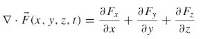
Figure 2-7 (a) Example of a divergence-free flux plot (incoming flux = outgoing flux); (b) flux plot with nonzero divergence (outgoing flux is greater than incoming flux, indicating that there are sources in the test region).
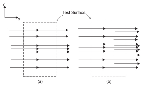
Figure 2-7a is an example of the flux plot for a divergence-free field. Inspection reveals why the divergence is zero because the vectors do not seem to converge or emerge from any source points. Additionally, a test closed surface (the box) placed in the region will have zero net flux emanating from it, because the flux lines going into the test region equal the flux lines leaving it. Figure 2-7b has nonzero divergence. Note that the emergence or convergence of the field vectors from source points is a common characteristic of a field with finite divergence. Simply put, if a region contains a source of a field, it will have a positive divergence. In Figure 2-7b, the nonzero divergence is evident from inspection because discontinuous flux lines are required to represent the increasing density with x, yielding a net nonzero flux. In other words, there are more flux lines emanating from the closed surface than are entering it, meaning that a source of the field must exist inside the test region.
An understanding of the meaning of divergence allows us to gain some insight into Gauss’s laws:
(2-3)![]()
(2-4)![]()
Note that the divergence of ![]() , which equals ε
, which equals ε ![]() , is nonzero and equal to the charge density, which implies that the source of the electric field is an electrical charge. Equivalently, if the electric field terminates abruptly, the termination must be an electric charge. Conversely, the divergence of
, is nonzero and equal to the charge density, which implies that the source of the electric field is an electrical charge. Equivalently, if the electric field terminates abruptly, the termination must be an electric charge. Conversely, the divergence of ![]() is zero, indicating that there is no magnetic equivalent to the electric charge and that the magnetic field is always source-free. For a test surface, the number of flux lines entering the surface must equal the flux leaving it, and there are no abrupt terminations ofthe magnetic field. Therefore, the flux lines of a magnetic field consist of closed lines.
is zero, indicating that there is no magnetic equivalent to the electric charge and that the magnetic field is always source-free. For a test surface, the number of flux lines entering the surface must equal the flux leaving it, and there are no abrupt terminations ofthe magnetic field. Therefore, the flux lines of a magnetic field consist of closed lines.
2.2.8 Curl
Historically, the concept of curl comes from a mathematical model of hydro-dynamics. Early work by Helmholtz studying the vortex motion of fluid led ultimately to Maxwell’s and Faraday’s conceptions of electric fields induced by time-varying magnetic fields, which is shown in equation (2-1) [Johnk, 1988]. To visualize the concept of the curl, consider a paddle wheel immersed in a stream of water, with a velocity field as shown in Figure 2-8. In Figure 2-8a, the paddle is oriented along the z-axis perpendicular to the water flow, and since the velocity of the fluid is larger on the top of the paddle, the paddle will rotate clockwise, and therefore has a finite curl along the z-axis, with a direction pointing into the page as determined using the right-hand rule. Similarly, if the paddle is rotated so that it is oriented along the x-axis, as in Figure 2-8b, the paddle will not rotate, and the curl is zero.
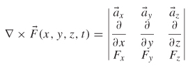
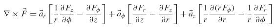
The curl of ![]() (x,y,z,t) in determinant form (in rectangular coordinates) is
shown as
(x,y,z,t) in determinant form (in rectangular coordinates) is
shown as
which simplifies to
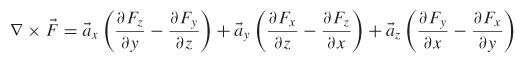
Figure 2-8 (a) The fluid velocity field causes the paddle wheel to rotate when it is oriented orthogonal to the field, giving it a nonzero curl with a direction pointing into the page (-z); (b) when the paddle wheel is parallel to the field it has a zero curl because the field will not make it rotate.
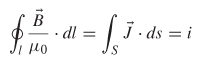
Simply put, if the curl is finite, a field will be induced that possesses circulation. This allows us intuitively to understand Faraday’s and Ampère’s laws:
Faraday’s law says that a time-varying magnetic field will induce an electric field that possesses circulation around ![]() . More intuitively, if we examine Ampère’s law for a steady-state current, it reduces to
. More intuitively, if we examine Ampère’s law for a steady-state current, it reduces to
Equation (2-25) implies that a current flowing in a wire will induce a magnetic field that circulates around the wire, which is consistent with Gauss’s law for magnetism (2-4), which implies that the flux lines of a magnetic field must consist of closed lines.
Example 2-2 Calculate the magnetic field of a current I flowing through an infinitely long wire of radius a. Show that the current flowing in the wire induces a magnetic field that circulates around the z-axis. See Figure 2-9.
SOLUTION To solve this problem it is necessary to present the integral form of Ampère’s law for static fields:
Switching to a cylindrical coordinate system, ![]() = aϕBϕ and dl = aϕrdϕ, yielding
= aϕBϕ and dl = aϕrdϕ, yielding
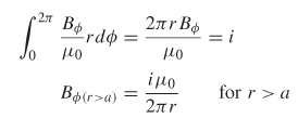
To calculate the magnetic field inside the conductor, only the amount of current passing through a percentage of the wire area must be considered. This is achieved by expressing the current in terms of an area ratio:
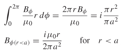
Figure 2-9 How the magnetic field will rotate around a wire carrying current.
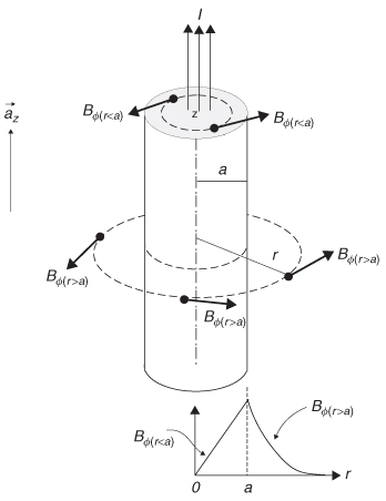
The analysis above shows that the magnetic field has only a ϕ-component that is perpendicular to the current flow, proving that the magnetic field will wrap around the wire. Since the current flow is inducing the magnetic field, its intensity will increase until r becomes greater than the wire radius a. When examining fields outside the wire radius (where no current is flowing), the magnetic fields will decrease, as shown in Figure 2-9.
We can confirm that ![]() circulates around the wire by calculating the curl. The curl of the magnetic field inside the wire can be calculated using the differential form of Ampère’s law for the static case:
circulates around the wire by calculating the curl. The curl of the magnetic field inside the wire can be calculated using the differential form of Ampère’s law for the static case:
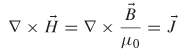
The curl of ![]() in cylindrical coordinate is (from Appendix A)
in cylindrical coordinate is (from Appendix A)
The solution of the integral form of Ampère’s law shows that the only component of the magnetic field in the ϕ-direction is a function of r. Consequently, the curl becomes
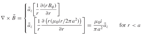
which says that the magnetic field with a ϕ-component will be induced that circulates around a wire when current I is flowing in the z-direction.
For r > a, the curl becomes
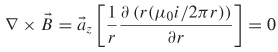
The curl of the magnetic field outside the wire is zero. This does not mean that the magnetic field does not circulate around the wire outside the conductor (it certainly does). The zero curl result is simply due to the fact that the area outside the conductor does not contain any current density (![]() = 0), and therefore Ampère’s law states that the curl of the magnetic field must be zero.
= 0), and therefore Ampère’s law states that the curl of the magnetic field must be zero.
2.3 WAVE PROPAGATION
When studying Maxwell’s equations, it becomes apparent that Faraday’s and Ampère’s laws (the two curl equations), which state, respectively, that a changing magnetic field will produce an electric field and a changing electric field will produce a magnetic field, are responsible for the propagation of an electromagnetic wave. In this section we derive equations that regulate electromagnetic wave propagation in a simple source-free medium. In the study of signal integrity, the propagation of waves in packages, on printed circuit boards, though cables, and between power and ground planes constitutes a very large portion of the discipline. In fact, communication between components in a high-speed digital design necessitates the intentional propagation of electromagnetic waves guided by transmission lines and the prevention of energy propagation across unintentional pathways (such as crosstalk) or in unwanted signal propagation modes. Without a detailed study of wave propagation, the study of signal integrity would become impossible.
2.3.1 Wave Equation
In subsequent chapters it will become necessary to analyze electromagnetic wave propagation only in terms of magnetic or electric fields because they are related directly to the voltage and current propagating on transmission lines, through vias, or across planes. The wave equation forms the basis for calculating critical electrical properties, such as crosstalk, reflections, standing waves, and different modes of propagation in multiconductor systems (e.g., a bus). We begin by manipulating Faraday’s and Ampère’s laws using some useful vector identities:
(2-1)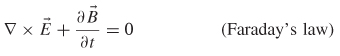
(2-2)![]()
Taking the curl of (2-1) produces

Since ![]() = μr μ0
= μr μ0 ![]() [from (2-8)], the equation above can be written in terms of the electric field by substituting (2-2) into the right-hand part:
[from (2-8)], the equation above can be written in terms of the electric field by substituting (2-2) into the right-hand part:
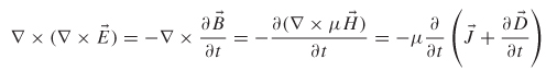
where μ= μr μ0.
If it is assumed that the region of wave propagation is source-free, the current density ![]() is zero. Combining equations (2-6) and (2-9) yields the relation
is zero. Combining equations (2-6) and (2-9) yields the relation ![]() = εrε0
= εrε0 ![]() = ε
= ε ![]() and allows the equation to be expressed only in terms of
and allows the equation to be expressed only in terms of ![]() :
:
![]()
The formula can be simplified further by using the following vector identity (see Appendix A):
![]()
Since we have assumed a source-free medium, the charge density is zero (ρ = 0), Gauss’s law reduces to ![]() ·
· ![]() = 0, yielding equation (2-27), which is known as the wave equation for the electric field:
= 0, yielding equation (2-27), which is known as the wave equation for the electric field:
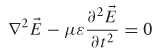
Using the identical technique, the wave equation for the magnetic field can be derived:
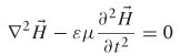
Note that equations (2-27) and (2-28) are similar except that the order of multiplication of με is reversed. The order of multiplication for this derivation was preserved because it will become important when using matrices to calculate the solution for waves propagating on multiple transmission lines in Chapter 4.
2.3.2 Relation Between E and H and the Transverse Electromagnetic Mode
The wave equations (2-27) and (2-28) are presented in their most general form, where the fields have components in four dimensions: x, y, z, and time. However, for the vast majority of signal integrity analysis, the wave equations (and all of Maxwell’s equations) can be simplified so that the fields have only one nonzero component that varies with one spatial coordinate. For example, the electric field ![]() (x, y, z, t) can be reduced to
(x, y, z, t) can be reduced to ![]() xEx(z, t). A good example of this is the magnetic field that was calculated in Example 2-2, where the magnetic flux intensity
xEx(z, t). A good example of this is the magnetic field that was calculated in Example 2-2, where the magnetic flux intensity ![]() had only one component in the ϕ-direction.
had only one component in the ϕ-direction.
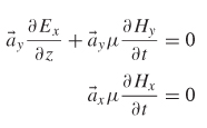
Although the wave equations (2-27) and (2-28) were derived separately, they are coupled and interdependent. For example, if the electric field is restricted so that ![]() =
= ![]() xEx(z,t), similar restrictions on the magnetic field cannot be chosen arbitrarily. In this case, since (2-27) was derived using the entire set of Maxwell’s equations, once the electric field is restricted, the magnetic field is already determined. Thus, the proper way to calculate the magnetic field is to derive it from the electric field. For example, if a wave is propagating in a source-free medium in the z-direction and its electric field only has a component in the x-direction [
xEx(z,t), similar restrictions on the magnetic field cannot be chosen arbitrarily. In this case, since (2-27) was derived using the entire set of Maxwell’s equations, once the electric field is restricted, the magnetic field is already determined. Thus, the proper way to calculate the magnetic field is to derive it from the electric field. For example, if a wave is propagating in a source-free medium in the z-direction and its electric field only has a component in the x-direction [![]() =
= ![]() xEx (z,t)], the magnetic field can be calculated from (2-1) and (2-2):
xEx (z,t)], the magnetic field can be calculated from (2-1) and (2-2):
(2-1)
Since we have restricted ![]() so that it varies only with z (
so that it varies only with z ( ![]()
![]() /(
/(![]() x = (
x = ( ![]()
![]() /(
/( ![]() y = 0), equation (2-24) shows that the curl of E can only produce components in the x- and y-directions.
y = 0), equation (2-24) shows that the curl of E can only produce components in the x- and y-directions.
Since ![]() = μ
= μ ![]() ,
,
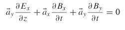
Grouping into vector components yields
From Ampère’s law (2-2),
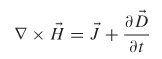
Figure 2-10 How the electric and magnetic fields are related as a TEM electromagnetic pulse propagates through space along the z-axis.
where ![]() = 0 for a source-free medium and
= 0 for a source-free medium and ![]() = ε
= ε ![]() (for now, we assume that
(for now, we assume that ![]() = 0):
= 0):
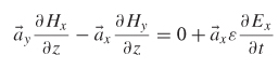
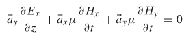
Grouping into vector components yields
The nonzero components of the equations above can be grouped to see the contributions in both the × - and y-directions.

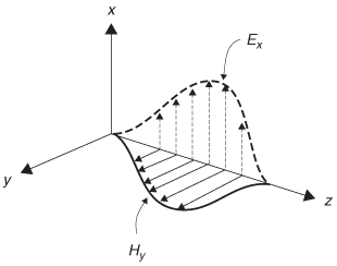
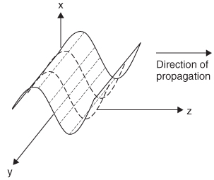
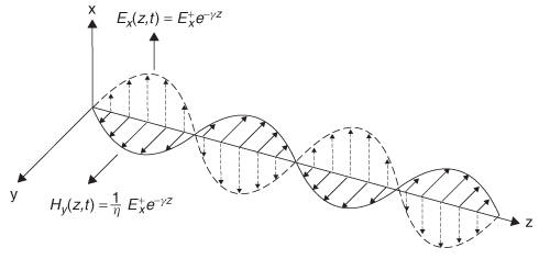
Equations (2-29) and (2-30) symbolize an important concept used throughout signal integrity analysis, which is that the electric and magnetic fields are orthogonal and there are no components in the z-direction. When waves propagate in this manner, it is called the transverse electromagnetic mode (TEM). Figure 2-10 depicts the relationship between the electric and magnetic fields as the TEM electromagnetic pulse propagates along the z-axis.
It should be noted that waves are not always restricted to propagate only in TEM mode because some structures (such as a microstrip) distort the waveform so that a small portion of the fields will have a z-component that lies outside the x - y plane. However, the relationship between the wavelength and the structure sizes in practical systems allows us to assume that the waves are propagating in TEM mode until very high frequencies. Measurements have confirmed that the TEM assumption remains valid to at least 50 GHz for typical transmission-line structures used in contemporary digital designs. The validity of the TEM assumption for transmission lines is discussed further in Chapter 3.
2.3.3 Time-Harmonic Fields
A simplification of Maxwell’s equations can be made if the time variation is assumed to be steady-state sinusoidal or time harmonic in nature. Although perfect sinusoidal waveforms are rarely encountered in digital design, the trapezoidal digital pulses usually employed can be constructed from a series of sinusoidal waveforms via the Fourier transform, making this general simplification partic-ularly useful. Time-harmonic electromagnetic fields will be generated whenever their charge and current sources also have densities that have a sinusoidal variation with time. Assuming that the sinusoidal sources are steady state permits the assumption that both ![]() and
and ![]() also reach steady state and vary according to cos(ωt + θE) and cos(ωt + θB), where ω = 2πf and θ is the phase of either the electric or the magnetic field.
also reach steady state and vary according to cos(ωt + θE) and cos(ωt + θB), where ω = 2πf and θ is the phase of either the electric or the magnetic field.
Generally, a sinusoidal waveform can be represented as
so the sinusoidal form of a time-harmonic field will vary according to the complex exponential factor ejωt, which leads to a reduction of Maxwell’s equations from a function space and time to simply space:
Equations (2-32) allow Maxwell’s equations to be rewritten as
The curl and the gradient affect only space-dependent functions, and the ejωt is operated on only by the partial time derivatives. Therefore, after canceling allthe extraneous ejωt terms, the time-harmonic form of Maxwell’s equations, where time has been eliminated, is shown.
Note that the time variation of the fields can be restored by multiplying by ejωt and taking the real part:
2.3.4 Propagation of Time-Harmonic Plane Waves
As will be demonstrated in subsequent chapters, the propagation of time-harmonic plane waves is of particular importance for the study of transmission-line or other guided-wave structures. This allows us to study a simplified subset of Maxwell’s equations where propagation is restricted to one direction (usually along the z-axis) and time is removed as described in Section 2.3.3. A plane wave is defined so that propagation occurs in only one direction (z) and the fields do not vary with time in the x- and y-directions. If the fields were observed at an instant in time, they would be constant in the x - y plane for any given point z and would change for different values of z or t. Figure 2-11 depicts a plane wave propagating in the z-direction.
To study the behavior of time-harmonic plane waves, it is necessary to re-derive the wave equation from the time-harmonic form of Maxwell’s equations using the procedure employed in Section 2.3.1. Again, assume a source-free, linear, homogeneous medium:
Figure 2-11 Plane wave propagating in the z-direction.
![]()
The formula can be further simplified by using the following vector identity (Appendix A):
![]()
Since we have assumed a source-free medium, the charge density is zero (ρ = 0) and Gauss’s law reduces to ![]() ·
· ![]() = 0, yielding
= 0, yielding
Substituting γ2 = ω2 με is yields
which is the time-harmonic plane-wave equation for the electric field, where γ is known as the propagation constant.
If the solution is limited to plane waves propagating in the z-direction that have an electric field component only in the x -direction, the wave equation becomes (see Appendix A)
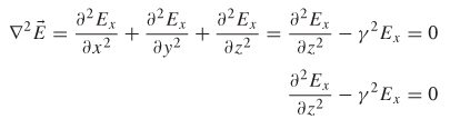
which is a second-order ordinary differential equation with the general solution
where C1 and C2 are determined by the boundary conditions of the particular problem.
As discussed in Chapter 3, equation (2-41) and its magnetic field equivalent will prove to be particularly important for signal integrity because they describe the propagation of a signal on a transmission line. The first term, C1e-γz, describes completely the forward-traveling part of the wave propagating in the z-direction (i.e., down the length of the transmission line), and the second term, C2 e+γz, describes the propagation of the rearward-traveling wave in the -z -direction. Observing equation (2-41) allows the definition of an important term, the propagation constant:
The terms in (2-42) have special meanings used throughout the book to describe the medium where the electromagnetic wave is propagating, whether it is in free space, is an infinite dielectric, or is a transmission line. Specifically, α is the loss term, which describes signal attenuation as it propagates through the medium. The loss term accounts for the fact that real-world metals are not infinitely conductive (except superconductors) and dielectrics are not perfect insulators (except free space), both of which are discussed in detail in Chapters 5 and 6. The imaginary portion of (2-42), β, called the phase constant, essentially dictates the speed at which the electromagnetic wave will travel in the medium. To visualize these waves propagating as described in (2-41), it is necessary first to recover the time dependency removed in Section 2.3.3. Considering only the forward-propagating component of a wave in a vacuum, replacing Ci with the magnitude of the electric field, restoring the time dependency as in (2-37), and applying the identity of equation (2-31) yields
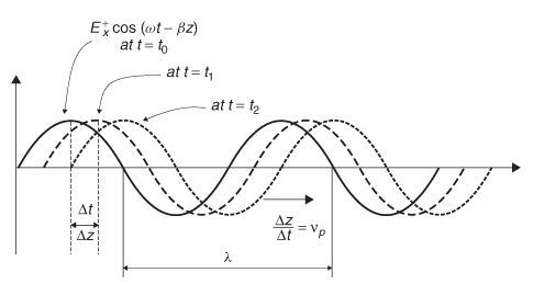
Assuming that the loss term is zero (α = 0), Figure 2-12 depicts successive snapshots of a wave propagating though space. To determine how fast the wave is propagating, it is necessary to observe the cosine term for a small duration of time Δt. Since the wave is propagating, a small change in time will be proportional to a small change in distance Δz, which means that an observer moving with the wave will experience no phase change because she is moving at the phase velocity (vp). Setting the term inside the cosine of (2-43) to a constant (ωt - βz = constant) and differentiating allows the definition of the phase velocity from the cosine term in (2-43):
Figure 2-12 Snapshots in time of a plane wave propagating along the z-axis, showing the definition of phase velocity.
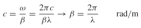
The relationship between the frequency and its wavelengths is calculated based on the speed of light, which is the phase velocity (vp) in a vacuum:

Since ω = 2πf and c is the speed of light in a vacuum (ca. 3 × 10⁸ m/s), equation (2-45) can be substituted into (2-44) to obtain a useful formula for β in terms of the wavelength λ:
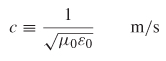
The speed of light in a vacuum is defined as the inverse of the square root of the product of the permeability and the permittivity of free space:
Calculation of λ in terms of (2-47) allows the phase constant β to be rewritten in terms of the properties of free space:
This is expanded on later in this chapter to include propagation of a wave in a dielectric medium.
Now that the propagation constant has been defined, (2-43) can be rewritten in physical terms, assuming free space (which is lossless, so α = 0):
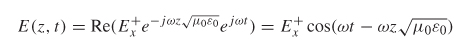
Since (2-49) is a solution to the wave equation, the magnetic field is found simply by using Faraday’s law (![]() ×
× ![]() + jωB = 0):
+ jωB = 0):
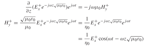
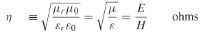
where η0 is the intrinsic impedance of free space and has a value of 377Ω
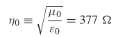
Equations (2-49) and (2-50) describe how a plane wave propagates in free space. The intrinsic impedance and the speed of light are constants that describe how the electromagnetic wave will propagate through the medium. The speed of light defines the phase delay of the wave, and the intrinsic impedance describes the relationship between the electric and magnetic fields. However, for wave propagation in other media, such as the dielectric of a printed circuit board (PCB), the speed of light and the intrinsic impedance are calculated using the relative permittivity εr and relative permeability μr, which simply describe the properties of the material relative to free-space values. Note that both μr and εr are unitless values that are real numbers for loss-free media but become complex for lossy media, as described in Chapters 5 and 6. The speed of light (referred to as the phase velocity for media other than free space) and the intrinsic impedance in a medium is calculated as
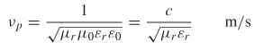
Note that for free space, μr and εr are both defined to be unity.
Equations (2-54) and (2-55) summarize the TEM plane waves of both the electric and magnetic fields in general form, with the time dependency removed:
where γ = a + j β is the propagation constant; α describes how the signal is attenuated by conductor and dielectric losses, described in full detail in Chapters 5 and 6; and β is the phase constant, as defined by (2-46) when the phase velocity in (2-52) is substituted for the speed of light in a vacuum (c). Note that the second term in (2-55) is negative. This is because the sign of the exponent for the reverse traveling wave does not cancel the negative sign in Faraday’s law as it did for the forward-traveling wave in equation (2-50) when the derivative with respect to z was calculated. The terms ![]() and
and ![]() describe the directions of each component of a propagating wave. For example, the total propagating wave could have a portion of the electric field propagating in the +z-direction and another propagating in the - z-direction. Figure 2-13 depicts a time-harmonic TEM plane wave propagating along the z-axis.
describe the directions of each component of a propagating wave. For example, the total propagating wave could have a portion of the electric field propagating in the +z-direction and another propagating in the - z-direction. Figure 2-13 depicts a time-harmonic TEM plane wave propagating along the z-axis.
2.4 ELECTROSTATICS
Electrostatics is the study of stationary charge distributions. A complete understanding of electrostatics is essential for the high-speed digital designer because it forms the basis of fundamental signal integrity theory and promotes an intuitive understanding of how electric fields behave. In this chapter we (1) define the electric field, (2) describe how energy is stored in the electric field, and (3) define capacitance, which is the circuit element used in circuit models to represent the energy stored in an electric field. The vast majority of signal integrity analysis performed in the industry today uses electrostatic techniques to calculate critical design variables such as transmission-line impedance, phase velocities, and effective dielectric permittivities. The concepts introduced in this section are expanded on in later chapters to describe a myriad of concepts.
Figure 2-13 Time-harmonic TEM plane wave propagating down the z-axis.
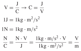
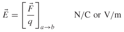
When a weightlifter hoists a barbell over his head, the energy expended (or the work done against the gravitational field) is stored in the form of potential energy. The gravitational potential energy can be recovered by lowering the barbell to the ground. Similarly, when two infinitely separated charges of the same polarity are brought together, the charges will experience a repulsive force whose magnitude depends on the distance between the charges. The existence of this force is described by saying that a charge q with units of coulombs (C) produces an electric field in the region surrounding it. When the electric fields of two charges of the same polarity begin to interact, a force will be generated that will push the charges apart. Therefore, the region surrounding a charge is permeated by a force field known as the electric field, defined fundamentally as force per unit charge, with units of newtons per coulomb (N/C). Note that because a volt is defined as joules per coulomb (J/C), newtons per coulomb is equivalent to volts per meter (V/m), which are the units commonly used to describe an electric field.
The description above makes the argument that an electric field is a field of force. If that force field acts upon a body to move it, work is done. The energy used to perform the work must either be dissipated by losses (friction in mechanical systems) or stored in the form of kinetic or potential energy. For example, if a test charge q is moved to different positions in an electric field produced by a fixed charge Q, either work must be performed to keep the charges separated (in the case of opposite charges) or work must be performed to bring the charges closer together (in the case of the same polarity charges). In this case, no energy is dissipated (in a loss-free system) because the energy in stored in the separated configuration and the energy can be recovered if the charges are allowed to return to the initial positions. The stored energy is potential energy because it depends on the position of the charges within the field. The concept of scalar electric potential, which will now be derived, provides a metric to describe the work or energy required to move charges from one point to another inside an electrostatic field.
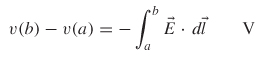
The discussion above describes how an electric field is produced when two charges are brought into the vicinity of each other. If we assume that one charge (Q) is stationary and the other charge (q) is moved toward the stationary charge from point a to point b, the work can be calculated as force × distance. To calculate the work done while moving the charge along a path, the following line integral is used:
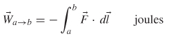
Note that the minus sign is necessary because (2-56) represents work being done against the field. The dot product accounts for the fact that it takes zero work to move the charge perpendicular to the field because there is no opposing force in that direction.
Since a fundamental unit of an electric field is newtons per coulomb (described above), the force field in (2-56) can be rewritten in terms of the electric field as
where q is a test charge being moved from point α to point b within the vicinity of a fixed charge Q, with units of coulombs. To calculate the electric field generated by a point charge, the integral form of Gauss’s law is used:
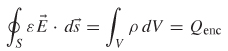
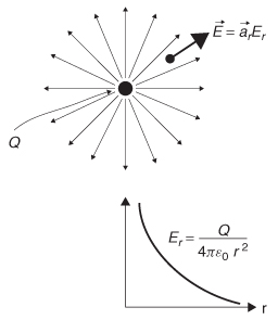
Figure 2-14 Electric field generated by a point charge Q.
where is the volume density of the charge within volume V in C/m3 and Qenc is the total charge enclosed by the surface S and contained in the volume V in units of coulombs.
As shown in Figure 2-14, a point charge has an electric field that radiates out in all directions, necessitating the use of spherical coordinates. In spherical coordinates, the ϕ and θ omponents of the electric field are zero, leaving only an r component directed outward from the point charge. Therefore, since the surface area of a sphere is 4πr2, the electric field around a point charge in free space is derived from (2-59):
Substituting (2-60) into (2-58) allows the calculation of the work done per unit charge when a charge is moved along r from point a to point b in an electrostatic field. Note that if the test charge was moved along ϕ or θ, there would be no work done because ![]() · d
· d![]() = 0; however, along the radial component,
= 0; however, along the radial component, ![]() · d
· d![]() = Erdr.
= Erdr.
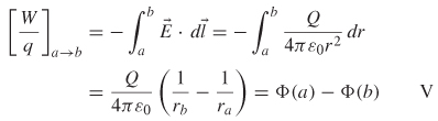
Therefore, we can define the electrostatic potential as work done to move a charge in an electrostatic field from point a to point b:
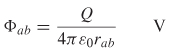
where rab denotes the radial distance that the stationary charge moved and Φab is known as the electrostatic potential or voltage between points α and b (don’t confuse the symbol for potential Φ with the polar coordinate variable ϕ).
2.4.1 Electrostatic Scalar Potential in Terms of an Electric Field
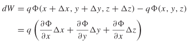
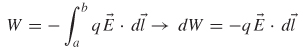
For electrical engineers, it is often convenient to think of fields in terms of more familiar circuit concepts, which are usually described in terms of potential differences (i.e., voltage) between points in a circuit. Therefore, a relationship between the electrostatic potential and the electric fields that is described in terms of a scalar function will prove to be useful in the study of signal integrity. To derive this relationship, it is convenient to sidestep the complexities of spherical coordinates and think in terms of simple rectangular coordinates. From equations (2-61) and (2-62) it is obvious that the differential amount of work done in moving a charge in an electrostatic field is directly proportional to the potential difference:
However, from equation (2-58),
In rectangular coordinates, d ![]() =
= ![]() xΔx +
xΔx + ![]() xΔy +
xΔy + ![]() zΔz. Thus, (2-63) can be simplified using the definition of the dot product in (2-13).
zΔz. Thus, (2-63) can be simplified using the definition of the dot product in (2-13).
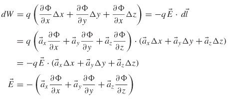
Note that the form of the last term in (2-64) is identical to (2-21), which is the gradient, which gives a very useful relation between the electric field and the electrostatic potential:
Also note that (2-65) can be derived using vector identities, which is significantly simpler but does not provide any intuition. The alternative derivation is shown here because we employ a similar technique when studying magnetostatics in the next section.
For an electrostatic field, Ampère’s law is reduced to ![]() ×
× ![]() = 0 because the field does not vary with time. For any differentiable scalar function, the following vector identity holds true (from Appendix A):
= 0 because the field does not vary with time. For any differentiable scalar function, the following vector identity holds true (from Appendix A):
![]()
Therefore, since ![]() ×
× ![]() = 0,
= 0, ![]() must be derivable from the gradient of a scalar function. Since (2-61) shows a relationship between the electrostatic potential and the electric field, a leap of logic says that the scalar function in the vector identity must be the electrostatic potential:
must be derivable from the gradient of a scalar function. Since (2-61) shows a relationship between the electrostatic potential and the electric field, a leap of logic says that the scalar function in the vector identity must be the electrostatic potential:
Equation (2-65), known as the electrostatic scalar potential, is used often when solving electrostatic problems such as transmission-line impedance or calculating the effective dielectric constant of a microstrip, as we demonstrate in Chapter 3.
2.4.2 Energy in an Electric Field
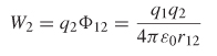
To calculate the energy stored in an electric field, it is necessary to begin with a stationary charge (q1) in free space that is infinitely far way from any other charges. It takes no work to move the first charge into position (W1 = 0) because there are no other nearby charges to provide electrostatic repulsion. Then we calculate how much work it takes to bring another charge (q2 ) into the vicinity of the first charge using (2-61) and (2-62):
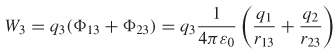
If we bring another charge, q3, into the vicinity of q1 and q2 , the work is calculated as
Thus, the total work done to bring the three charges together is
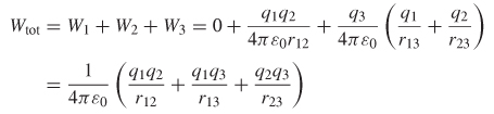
which can be generalized into the following double summation to account for n charges:
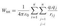
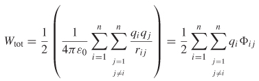
The limit on the j term exists to ensure that terms are not counted twice. For example, without the limit the term Φ12 would be counted twice because Φ12 = Φ21, which simply means that it takes the same amount of work to move q1 into the vicinity of q2 as it does to move q2 into the vicinity of q1. Equation (2-68) can be simplified by allowing the terms to be counted twice and dividing by 2 to compensate for the double counting of terms:
Equation (2-69) is the work it takes to assemble n charges. It is interesting to consider where the energy is stored in an accumulation of charges. It is analogous to a mechanical system of a compressed spring with a weight on each end. If the weights are forced together, the energy is stored in the stressed state of the spring. Therefore, just like the spring example, the charges, which will tend to repel each other, will have stored energy that is a function of the proximity of the charges and the properties of an electric field.
To calculate the energy stored in a continuous charge distribution, and thus an electric field, it is more convenient to express the charge in terms of the unit volume, the potential in terms of a continuous function, and to take the limit as n → ∞ ), which allows us to write (2-69) in terms of an integral,
where ρ (r) is the charge density in units of C/m3.
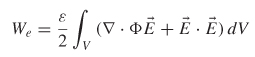
It is useful to express (2-70) in terms of the electric field. To do this, Gauss’s law is used to express the charge density in terms of the electric field:
This equation can be simplified using the flowing vector identity (Appendix A):
![]()
The identity can be rewritten in terms of the electrostatic vector potential, substituting ψ = Φ and ![]() = ε
= ε ![]() :
:
![]()
Since ![]() = -
= - ![]() Φ, the equation can be simplified further:
Φ, the equation can be simplified further:
The divergence theorem of vector calculus states (Appendix A) that
![]()
allowing further simplification of (2-72):
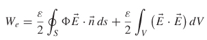
where ![]() is a unit vector normal to the surface.
is a unit vector normal to the surface.
Equation (2-73) describes the total energy in an electric field that is induced by a volume of charges. If we expand the volume of integration to include all space, any contribution of (2-73) outside the charge distribution will contribute nothing to the work done since there are no charges in that space. Also note that if the volume of integration is chosen to be infinity, the surface integral disappears. To understand why, remember that the surface integral sums all the contributions evaluated at the surface. Since ![]() [equation (2-62)], E
[equation (2-62)], E ![]() 1/r2 [equation (2-60)], and ds
1/r2 [equation (2-60)], and ds ![]() r2, the limit of F
r2, the limit of F ![]() ·
· ![]() ds is pro-portional to (1/r)(1/r2)r2, whose limit goes to zero when r is infinity and the surface integral disappears. The volume integral includes contributions over the entire volume, not only on the surface. Subsequently, equation (2-73) can be reduced to (2-74), which is the work done by accumulating charges to create an electric field:
ds is pro-portional to (1/r)(1/r2)r2, whose limit goes to zero when r is infinity and the surface integral disappears. The volume integral includes contributions over the entire volume, not only on the surface. Subsequently, equation (2-73) can be reduced to (2-74), which is the work done by accumulating charges to create an electric field:
This leads to the definition of the volume energy density, which expresses the stored energy in a charge distribution in terms of the electric field:
2.4.3 Capacitance
In circuit terms, the quantity associated with storing energy in an electric field is capacitance. To define capacitance, imagine two conductors, with a charge of +Q on one and of -Q on the other. If we assume that the voltage is constant over each conductor, the potential difference (voltage) between them is calculated as
We show that ![]() is proportional to Q:
is proportional to Q:
Since ![]() is proportional to both Q and v, we can define a constant of proportionality that relates Q and v. The constant of proportionality is defined to be the capacitance :
is proportional to both Q and v, we can define a constant of proportionality that relates Q and v. The constant of proportionality is defined to be the capacitance :
where Q is the total charge in coulombs and v is the voltage potential between the conductors, given in units of farads, defined as 1 coulomb per volt. Capacitance depends purely on the geometry of the structures and the value of the dielectric permittivity. Note that v is defined as the potential of the positive conductor minus the negative conductor and that Q is the charge on the positive conductor. Therefore, capacitance is always a positive value.
Example 2-3 Consider the case where two conductive plates of area α are oriented parallel to each other separated by a distance d. Assume that we place a charge of +Q on the top plate and -Q on the bottom plate and assume that the charges will spread out evenly (a reasonable assumption, assuming a good conductor). Then the surface charge density becomes
![]()
SOLUTION Using the integral form of Gauss’s law (2-59), we can calculate the electric field:
where dV in this case refers to the volume. Since we are considering the charge distribution on a surface, d ![]() = dV =
= dV = ![]() A (where
A (where ![]() is the unit normal vector to the plate), we can write the electric field in terms of the area and dielectric permittivity:
is the unit normal vector to the plate), we can write the electric field in terms of the area and dielectric permittivity:
The voltage is evaluated with equation (2-58), where dl = x(a) - x(b) = d, which is the distance between the plates:
Therefore, the capacitance between two parallel plates is
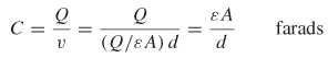
where A is the area of the parallel plates, v the voltage, and d the distance between them.
2.4.4 Energy Stored in a Capacitor
The process of storing energy in a capacitor involves electric charges of equal magnitude, but opposite polarity, building up on each plate. As long as the capacitor holds a charge, it is storing energy. To calculate how much energy is stored in a capacitor, consider how much energy it would take to transport a single charge from the positive plate to the negative plate. From equation (2-58) we know that voltage is the work done to move a charge from point a to b,
and capacitance is defined as
![]() (2-76)
(2-76)
Therefore, the amount of work needed to move one charge q of the total charge Q from plate α to plate b is
![]()
To calculate the total work done to charge up the capacitor to a value of Q, all charges must be moved:
However, from (2-69), Q = Cv. Therefore, the energy stored in a capacitor with a final potential of v is
2.5 MAGNETOSTATICS
In Section 2.4 we discussed the problem of classical electrostatics, where we defined the electric field in terms of the force that a collection of charges exert on each other. In the case of electrostatics, we considered only cases where the charges are at rest. Now it is time to consider the forces that exist between charges in motion.
To begin this discussion, let’s consider an experiment that most people performed in high school physics class. If you recall, direct current (dc) (from a battery) driving through a coil will produce an electromagnet. The magnetic field produced by such a configuration can be descried by Ampère’s law, ![]() ×
× ![]() =
= ![]() . Note that the time dependence of the electric field (
. Note that the time dependence of the electric field ( ![]() D/
D/![]() t) has been eliminated because we are considering only a dc flow. Ampère’s law tells us that a steady-state current
t) has been eliminated because we are considering only a dc flow. Ampère’s law tells us that a steady-state current ![]() will induce a magnetic field
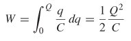
will induce a magnetic field ![]() that circulates around the wire. As described in Example 2-2, the direction of the circulation can be determined using the right-hand rule. If the thumb points in the direction of the current flow, the fingers of the right hand will curl around in the direction of the magnetic field. Subsequently, it is easy to imagine the form of the magnetic field from a single loop of current in our electromagnet, as shown in Figure 2-15a.
that circulates around the wire. As described in Example 2-2, the direction of the circulation can be determined using the right-hand rule. If the thumb points in the direction of the current flow, the fingers of the right hand will curl around in the direction of the magnetic field. Subsequently, it is easy to imagine the form of the magnetic field from a single loop of current in our electromagnet, as shown in Figure 2-15a.
Now consider a tiny elemental loop of current circulating around a point that will induce a small magnetic field as shown in Figure 2-15b. This small current loop will produce a small magnetic field that is analogous to an electric charge. In fact, historically, scientists initially speculated that there was a magnetic charge analogous to the electric charge described earlier. However, experimental evidence suggests overwhelmingly that magnetic charges do not exist. Magnetic fields are not generated by the forces that magnetic charges exert on each other; rather, magnetic fields are generated by current loops.
Similar to our description of the forces between charges in electrostatics, consider an isolated tiny current loop (l0) which will induce a magnetic field and behave like a small electromagnet. Now, bring another tiny current loop (l1) from infinity into the magnetic field of l0. If the orientations of the current loops are similar, it will take work to push them together because magnets exert forces on one another similar to electric charges. Like poles will repel each other, and unlike poles will attract. Each “electromagnet” has its own north and southpoles. It is interesting to note that the fundamental source of the magnetic field is the moving charge Q that constitutes the steady-state current. Subsequently, when l1 is moved into the proximity of lo, the force induced between the two electromagnets is caused by the charge (Q) of l1 moving in the magnetic field of lo and is described by the Lorenz force law:
Figure 2-15 (a) Magnetic field generated by a loop of current; (b) elemental current loop analogous to an electric charge.
A charge moving in the presence of both an electric and a magnetic field produces a force calculated as
The implications of (2-78) are that the force is perpendicular to both the velocity ![]() of the charge q and the magnetic field
of the charge q and the magnetic field ![]() . The magnitude of the force is F = qvB sin θ, where θ is the angle between the velocity vector and the magnetic field. Because sin(0) = 0, this implies that the magnetic force on a stationary charge or a charge moving parallel to the magnetic field is zero.
. The magnitude of the force is F = qvB sin θ, where θ is the angle between the velocity vector and the magnetic field. Because sin(0) = 0, this implies that the magnetic force on a stationary charge or a charge moving parallel to the magnetic field is zero.
From the force relationship in (2-78) it can be deduced that the units of magnetic field are newton · seconds/coulomb · meter or newtons/ampere · meter. This unit is named the tesla. It is a large unit, and the smaller unit gauss is used for small fields such as Earth’s magnetic field. A tesla is 10,000 G. Earth’s magnetic field is on the order of 0.5 G.
To make this concept more apparent, the force can be defined in terms of the current, which is the flow of 1 C of charge per second:
If we consider the current flowing along on a differential slice of a wire (dl), we can write (2-78) in terms of the current. Since Qv has units of C (m/s), which is the same as A · m, Qv can be simplified to I dl:
This allows us to write the force in terms of both the current and the magnetic field:
Equation (2-80) says that the force caused by the magnetic field will be perpendicular to the current flow and the magnetic field.
When deriving the energy in an electric field in Section 2.4, we calculated the amount of work done against the electric field to bring an accumulation of charges together. However, when calculating the energy in the magnetic field, a different approach must be taken because of a unique feature of equation (2-78).If a charge Q moves an amount d ![]() =
= ![]() dt in a magnetic field, the amount of work done is
dt in a magnetic field, the amount of work done is
Note that ![]() ×
× ![]() is perpendicular to the flow of the current, which follows the path of d
is perpendicular to the flow of the current, which follows the path of d ![]() . In other words, the work done by the magnetic field is zero because the force is perpendicular to the moving charge. Therefore, the magnetic field can change the direction of the moving particle, but it cannot speed it up or slow it down. This concept may be confusing, especially when considering the simple electromagnets that we all played with in high school, because we all know that we can use an electromagnet to pick up a paper clip. Since we are moving the mass of the paper clip against Earth’s gravitational field, we know that work is being done. However, if the work is not being done by the magnetic field, what is doing the work? The answer is demonstrated in the following example.
. In other words, the work done by the magnetic field is zero because the force is perpendicular to the moving charge. Therefore, the magnetic field can change the direction of the moving particle, but it cannot speed it up or slow it down. This concept may be confusing, especially when considering the simple electromagnets that we all played with in high school, because we all know that we can use an electromagnet to pick up a paper clip. Since we are moving the mass of the paper clip against Earth’s gravitational field, we know that work is being done. However, if the work is not being done by the magnetic field, what is doing the work? The answer is demonstrated in the following example.
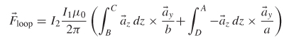
Example 2-4 Consider a long wire carrying current I1 in the presence of a rigid rectangular loop carrying current I2, as shown in Figure 2-16. The long wire will generate a magnetic field as calculated in Example 2-2:
![]()
Calculate the magnetic force.
Figure 2-16 Forces generated on a wire loop in the vicinity of a magnetic field generated from a wire.
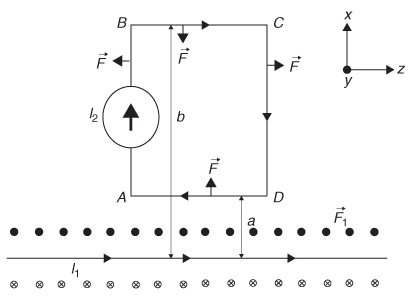
SOLUTION According to equation (2-80), the force exerted on the loop carrying current I2 in the presence of ![]() 1 is
1 is
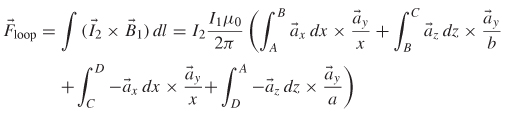
Note that the segments AB and CD are equal but opposite, so they cancel.
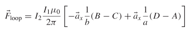
From the right-hand rule, the cross products are as follows:
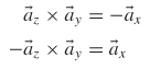
Therefore, the force is reduced to
Since segments BC - DA, we can call this length d
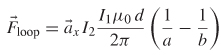
Therefore, the loop will be pushed away from the wire in the direction of ![]() x.
x.
Note that the magnetic force has caused the wire loop to move. Since work is force × distance, it would be easy to conclude that the magnetic force has performed work. However, equation (2-81) explicitly states that the magnetic field can do no work. What is performing work? To answer this question, consider the force vector on a single segment of the loop as soon as it begins to move. Remember that the force is perpendicular to the direction of the current flow, and the current flow is defined by the movement of charge. When the loop moves, the direction of the current flow 12 will be altered. To understand this, Figure 2-17 shows that the direction in which a single charge in the loop will travel when the loop is moved in the +x -direction. Instead of moving from right to left, it is moved up and to the left because the loop is moving in the +x -direction. This will cause the force vector, which must remain perpendicular to the current flow, to tilt to the right, as shown in Figure 2-17. When the force vector tilts, the component ![]() zFz opposes the charge flow of the current 12 in the loop. For 12 to remain constant, the source of the current must overcome this force. This leads us to the conclusion that the power source is performing the work! The magnetic field simply alters the direction of the force vector.
zFz opposes the charge flow of the current 12 in the loop. For 12 to remain constant, the source of the current must overcome this force. This leads us to the conclusion that the power source is performing the work! The magnetic field simply alters the direction of the force vector.
Figure 2-17 Forces generated on a wire loop in the vicinity of a magnetic field generated from a wire.

2.5.1 Magnetic Vector Potential
Because magnetic fields can do no work, we cannot calculate the energy stored in a magnetic field in the same manner as we did for the electric field (i.e., by calculating the work done to accumulate a distribution of elemental current loops), so another approach is needed. In this section we develop the concept of the magnetic vector potential. The magnetic vector potential is used to calculate inductance, which is in turn used to calculate the energy stored in a magnetic field.
The basic laws that rule magnetostatics are the time-invariant forms of Ampère’s and Gauss’s laws for magnetism:
If the following vector identity is applied (from Appendix A),
![]()
it implies that ![]() can be written in terms of the curl of a vector
can be written in terms of the curl of a vector ![]() . This is called the magnetic vector potential, which sometimes helps to simplify calculations such as inductance:
. This is called the magnetic vector potential, which sometimes helps to simplify calculations such as inductance:
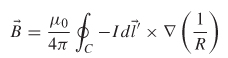
To calculate the form of ![]() , it is first necessary to introduce the most basic law of magnetostatics, the Biot-Savart law, which describes how the
, it is first necessary to introduce the most basic law of magnetostatics, the Biot-Savart law, which describes how the ![]() field at a given point is produced by the moving charges in the vicinity of that point. During application of this law, we consider currents that are either static or very slowly varying with time. The Biot-Savart law is given by [Inan and Inan, 1998]
field at a given point is produced by the moving charges in the vicinity of that point. During application of this law, we consider currents that are either static or very slowly varying with time. The Biot-Savart law is given by [Inan and Inan, 1998]
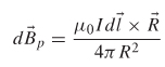
where I is the current, ![]() a unit vector pointing from the location of the differential current element Id
a unit vector pointing from the location of the differential current element Id ![]() to the point P, and R =
to the point P, and R = ![]() the distance between the current element and point P. Note that a primed quantity represents the position vector or the coordinates of the source points and the unprimed quantities represent the position vector or the coordinates of the point where
the distance between the current element and point P. Note that a primed quantity represents the position vector or the coordinates of the source points and the unprimed quantities represent the position vector or the coordinates of the point where ![]() is being evaluated. Note that the cross product in (2-84) indicates that d
is being evaluated. Note that the cross product in (2-84) indicates that d ![]() is perpendicular to both Id
is perpendicular to both Id ![]() and
and ![]() , with the orientation being described by the right-hand rule. Also note that the field generated by Id
, with the orientation being described by the right-hand rule. Also note that the field generated by Id ![]() will fall off with the square of the distance.
will fall off with the square of the distance.
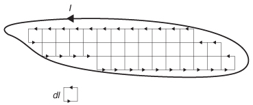
Note that the current element Id ![]() is a small part of a closed current loop and that an arbitrarily shaped loop can be constructed by the superposition of many such closed elemental loops of current, as shown in Figure 2-18. Subsequently, the Biot-Savart law can be written in terms of an integral:
is a small part of a closed current loop and that an arbitrarily shaped loop can be constructed by the superposition of many such closed elemental loops of current, as shown in Figure 2-18. Subsequently, the Biot-Savart law can be written in terms of an integral:
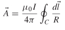
Careful observation of (2-85) allows us to calculate the form of the magnetic vector potential ![]() . Equation (2-83) states that the magnetic field is the curl of
. Equation (2-83) states that the magnetic field is the curl of ![]() . The trick is to manipulate (2-85) into the form of a curl so that
. The trick is to manipulate (2-85) into the form of a curl so that ![]() can be found. The right-hand term of (2-85) has a term that can be equated to the gradient of 1/R in spherical coordinates (see Appendix A):
can be found. The right-hand term of (2-85) has a term that can be equated to the gradient of 1/R in spherical coordinates (see Appendix A):
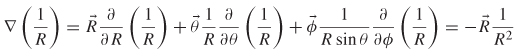
Figure 2-18 Any current loop can be constructed from many elemental current loops dI.
Substituting (2-86) into (2-85) gives
The del operator (![]() ) does not operate on source variables and therefore does not affect Id
) does not operate on source variables and therefore does not affect Id ![]() . Therefore, it is acceptable to rewrite (2-87) in the form of a curl:
. Therefore, it is acceptable to rewrite (2-87) in the form of a curl:

Also note that the negative sign has been eliminated because it indicates current direction, which is comprehended by the vector Id ![]() . Comparing (2-88) to the definition of the magnetic vector potential in (2-83), we can deduce the form of
. Comparing (2-88) to the definition of the magnetic vector potential in (2-83), we can deduce the form of ![]() :
:
2.5.2 Inductance
Suppose that two current loops are in close proximity to each other as shown in Figure 2-19. If a steady-state current (I1 ) is flowing in loop 1, it produces a magnetic field B1, as predicted by (2-85). If some of the magnetic field lines pass though loop 2, the flux passing through loop 2 is calculated using the form of equation (2-17):
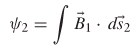
Note that the flux in loop 2 is proportional to ![]() l and is therefore also proportional to I1. This allows us to define a constant of proportionality, more commonly known as the mutual inductance:
l and is therefore also proportional to I1. This allows us to define a constant of proportionality, more commonly known as the mutual inductance:

Substituting the (2-83) into (2-90) gives the flux passing through loop 2 in terms of the magnetic vector potential, where S2 is the surface enclosed by loop 2:
Now we can simplify using Stokes’ theorem and substitute (2-89) for ![]() [Jackson, 1999]:
[Jackson, 1999]:
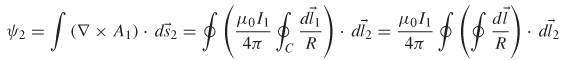
Figure 2-19 Mutual inductance caused by magnetic flux from loop 1 passing though loop 2.

Since ψ2 = L21 I1 [from (2-91)], the mutual inductance between loops 1 and 2 is determined by dividing (2-93) by the current in loop 1:
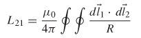
Equation (2-94), called the Neumann formula, involves integration around both loops 1 and 2. Note two very important concepts that can be derived from equation (2-94).
1. The mutual inductance is a function of the size, shape, and distance between the two loops.
2. The mutual inductance from loop 1 to loop 2 (L21) is identical to the mutual inductance from loop 2 to loop 1 (L12).
If we consider the implications of Faraday’s law (![]() ×
× ![]() +
+ ![]()
![]() /
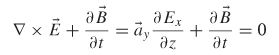
/ ![]() t = 0), another very important concept used throughout signal integrity can be surmised. For simplification, let’s assume that we only have a component of the electric field in the x-direction and it is propagating along z so that
t = 0), another very important concept used throughout signal integrity can be surmised. For simplification, let’s assume that we only have a component of the electric field in the x-direction and it is propagating along z so that ![]() =
= ![]() xEx(z, t). Faraday’s law is then reduced to
xEx(z, t). Faraday’s law is then reduced to
Equation (2-95) says that a time-varying magnetic flux ![]() generated from loop 1 and passing through loop 2 will induce an electric field and subsequently a voltage in loop 2. Faraday’s law can be rewritten in terms of circuit parameters:
generated from loop 1 and passing through loop 2 will induce an electric field and subsequently a voltage in loop 2. Faraday’s law can be rewritten in terms of circuit parameters:
Figure 2-20 Voltage sources induced by the time-varying currents in loop 1.
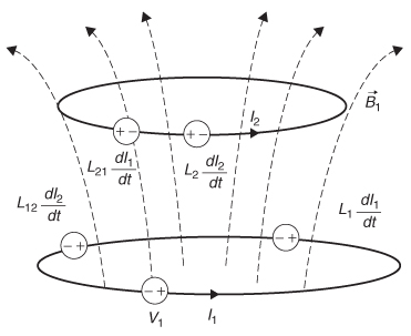
Therefore, every time you change the current in loop 1, an electromotive force (i.e., a voltage) is induced in loop 2, which causes current to flow. In addition to inducing a voltage on loops in the vicinity, changing current in loop 1 will change the magnetic flux flowing through itself and, consequently, induce a voltage in itself. This is called the self-inductance:

Similar to the mutual inductance, if the current changes a voltage is induced in the loop:
By observing (2-98), the units of inductance are determined to be volt · seconds per ampere, also known as henries. Figure 2-20 shows the voltage elements superimposed on the magnetically coupled loops corresponding to the mutual and self-inductance values calculated with (2-96) and (2-98). Note that the voltage sources were chosen to be positive and the negative sign is accounted for with the direction of current flow.
Example 2-5 Equivalent Circuit of a Magnetically Coupled System The magnetically coupled circuit can be understood more easily if conventional circuit theory is applied. Figure 2-21 shows the circuit for the magnetically coupled loops, assuming that the second loop is terminated in a resistor RL and each wire has a resistance of Rw. Kirchhoff’s voltage relations can be written for each loop:
Figure 2-21 Circuit for Example 2-5, showing magnetically coupled loops.
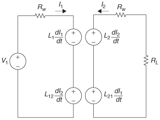
Loop 1:
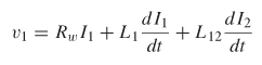
Loop 2:
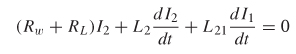
Note that inductance is always a positive quantity that can be compared to a mass in a mechanical system. Large masses are difficult to move, making it difficult to accelerate in any direction. Similarly, the greater the inductance, the more difficult it is to change the current because of the back emf (back voltage) generated in a direction to oppose the current, which is enforced by the negative sign in (2-98). This is called Lenz’s law.
2.5.3 Energy in a Magnetic Field
If a circuit has a finite amount of inductance, it takes energy to make a current flow because it requires work to overcome the back EMF voltage described by Lenz’s law. The work done on a charge against this back EMF is - v, from (2-98). The negative sign dictates that it is work being done against the EMF, not work done by the EMF. Since current is charge flow per unit time, the work done per unit time is derived from (2-58) and given by
Integrating the second half of (2-99) will provide the total work done and thus energy in the magnetic field in terms of the current and the inductance:
Note that (2-100) only depends on the loop geometry (which is where the inductance comes from) and the steady-state current.
It is often useful to represent the total energy in terms of the magnetic field. To translate inductance, which is a circuit quantity to a field quantity, equation (2-97) is used.
Recalling equations (2-90) and (2-92) and invoking Stoke’s theorem as in (2-93), the flux can be equated as follows:
Therefore, the work calculated in (2-100) can be rewritten
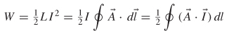
Expressing (2-103) in a volume integral allows us to use Ampère’s law (![]() ×
× ![]() / μ0 =
/ μ0 = ![]() ) in place of I:
) in place of I:
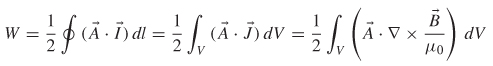
Conjuring up more mathematical trickery from Jackson [1999] allows us to rewrite (2-104) in a simplified form using the following vector identity:
Rearranging the terms and utilizing the definition of the vector magnetic potential,
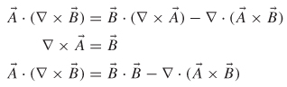
allows the work to be expressed in terms of the magnetic fields:
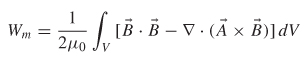
which can be simplified:
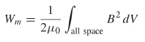
This leads to the definition of the volume energy density, which expresses the stored energy in a magnetic field:

2.6 POWER FLOW AND THE POYNTING VECTOR
As electromagnetic waves propagate through space, they carry power. The goal of this section is to derive a relationship between the electric and the magnetic field vectors and the power transferred. To begin this derivation, the energy stored in both the electric and magnetic fields must be quantified within a volume of space. Consider Figure 2-22, which depicts a cubic volume of space with an electromagnetic plane wave propagating through it. To quantify the total power, which is the transfer of energy over time, propagating through the cube, all sources of energy must be accounted for. The power balance equation can be expressed as
where PA is the power flowing through the surface of the far end of the cube of space with area A, as shown in Figure 2-22, PS represents any sources of power within the cube, PL represents the losses within the cube that dissipate power as heat (such as resistive losses), and PEM represent the power contained within the electromagnetic waves that propagate into the cube. If we assume a source-free and loss-free medium, the power flowing into the cube must equal the power flowing out of the cube, where the minus sign convention is chosen because the power is flowing out of the surface:
Figure 2-22 Volume of space used to calculate power flow and the Poynting vector.
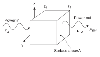
To quantify (2-109) in terms of the electric and magnetic fields, we begin with the volume energy densities for an electric and a magnetic field, which were derived earlier and listed here for convenience.
Integrating the sum of (2-75) and (2-107) over the volume of the cube will give total energy:
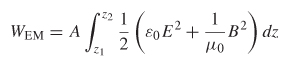
Since power is energy transfer per unit time interval, PEM is calculated by taking the time derivative:
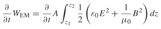
Defining the fields in time-harmonic form lets us express (2-111) in terms of the partial time derivatives:
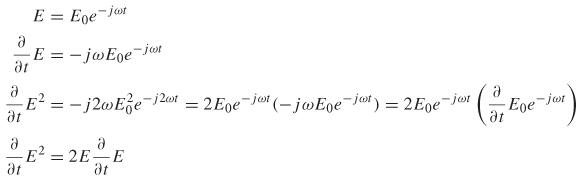
Similarly,
which allows (2-111) to be rewritten as
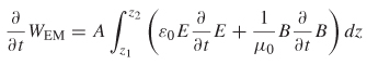
Now, for a plane wave propagating in the z-direction, the contributions of the fields in the y-direction were calculated earlier with equation (2-29):
and the contributions in the x-direction are given by
Note that ![]() = 0 since it is assumed that there are no sources in the volume under consideration.
= 0 since it is assumed that there are no sources in the volume under consideration.
Substituting (2-29) and (2-30) into (2-112) allows us to simplify the equation:
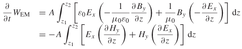
Note that the form of the integrand in (2-113) looks like a curl multiplied by a vector. This tells us that (2-113) might be simplified if we use the vector identity introduced earlier:
(2-105)![]()
Note that from (2-24), ![]() x(
x( ![]() Hy/
Hy/ ![]() z) = -
z) = - ![]() ×
× ![]() and
and ![]() y(
y( ![]() Ex/
Ex/ ![]() z) =
z) = ![]() ×
× ![]() . Therefore,
. Therefore,
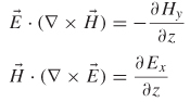
This allows us to rewrite (2-113) in terms of the cross product of the electric and magnetic fields:

Note that the final term in (2-114) is equivalent to a volume integral, where Adz = dV. This allows us to use the divergence theorem to eliminate the del operator:
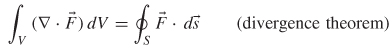
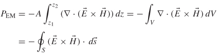
This allows us to define the Poynting vector, which represents the flow of power per unit area through a surface S at an instant in time.
Note that the direction of the power flow is perpendicular to both ![]() and
and ![]() .
.
2.6.1 Time-Averaged Values
When considering the electromagnetic power delivered by a sinusoidal time-varying field, practical measurement considerations tend to favor the time-averaged value of the power rather than the instantaneous value described in (2-115). This is because the time-averaged power entering a passive network, as measured with a watt-meter, is a measure of the power dissipated by heat in all the resistive circuit elements. In the laboratory, the time average of a time-harmonic function is taken over an interval of many periods. For a steady-state sinusoidal function, the average of one period will be the same as the average over many periods, since each period looks identical. The time average of the Poynting vector is defined as the area under the function for one period, divided by the duration of the cycle:
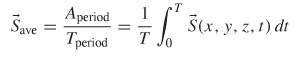
Although the math is not shown here, Jackson [1999] shows the derivation of the time average value for the Poynting vector:
where the star represents the complex conjugate.
It is sometimes useful to represent the magnitude of the Poynting vector in terms of the electric or magnetic fields and the intrinsic impedance defined in equation (2-53). Integrating sinusoidal functions as described in (2-116) will yield the time-averaged Poytning vector in terms of the ![]() and
and ![]() fields [Johnk, 1988]:
fields [Johnk, 1988]:
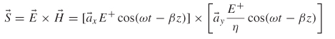
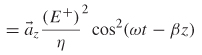
To obtain the time-averaged value of (2-120), remember that sin2 θ + cos2 θ = 1. Therefore, over a complete cycle, the average of cos2 θ is equal to the average of sin2 θ and sin2 θ = cos2 θ =½ Subsequently, the time-averaged value of a cosine-squared term over a complete cycle is ½:
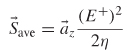
Similarly, the Poynting vector can be expressed in terms of the magnetic field:
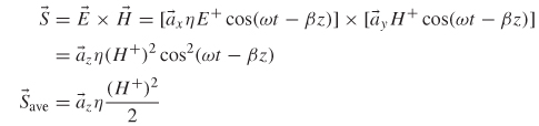
2.7 REFLECTIONS OF ELECTROMAGNETIC WAVES
So far, we have considered the propagation of electromagnetic waves in a simple, infinitely large medium. However, most practical problems involve waves propagating in multiple dielectric media. Since each medium will have different electric characteristics, it is essential to understand how a propagating electromagnetic wave will behave when it enters a region where the properties of the medium change.
Generally, when an electromagnetic plane wave propagating in medium A enters region B, where the properties of the dielectric change, two things happen: (1) a portion of the wave is reflected away from region B, and (2) a portion of the wave is transmitted into region B. When these plane waves encounter planar interfaces, both the reflected and transmitted waves are also planar, so their directions, amplitudes, and phase constants can easily be calculated. The simultaneous existence of both the transmitted and reflected waves is a direct result of the boundary conditions that must be satisfied when solving Maxwell’s equations at the interface between the two regions. We begin with a plane wave incident on a perfect conductor.
2.7.1 Plane Wave Incident on a Perfect Conductor
Consider a plane wave propagating in medium A in the z-direction. Assume that the medium in region α is a simple, loss-free medium and medium B is a perfectly conducting metal plane, as shown in Figure 2-23. Assume that the electric field is oriented in the x -direction, necessitating that the magnetic field
Figure 2-23 Incident electromagnetic wave propagating in dielectric region α and impinging on a perfect conductor.
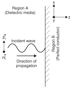
be oriented in the y-direction. The incident fields propagating in medium α are given by
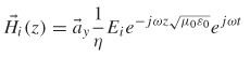
Since the boundary is normal to the incident waves, the reflected portion will be reflected back in the -z-direction. Subsequently, the reflected electric field will have the form
Since the electric field of the reflected wave is propagating in the -z-direction, the magnetic field must also flip and point in the -y -direction, to maintain the proper relationship between the electric and magnetic fields:
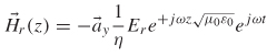
To calculate the values of the reflected and transmitted waves we must consider what happens when an electromagnetic field impinges on a perfect conductor. Equation (2-7) implies that an electric field impinging on a conductor with conductivity α will produce a current density ![]() :
:
(2-7)![]()
For a perfect conductor, σ = ∞. However, since the real world limits currents to finite densities, equation (2-7) implies that infinite conductivity will produce infinite currents inside a perfect conductor, which is impossible; therefore, the electric field inside the perfect conductor must be zero. If the electric field is zero, the magnetic fields must also be zero. This allows us to deduce the boundary conditions for both ![]() and
and ![]() at the interface between a dielectric medium and a perfect electrical conductor (PEC). Since the fields in region α are finite and the fields in region B (the PEC) are zero, we can deduce that the wave impinging on the conductor must induce a wave equal but opposite to the incident wave at the surface, so the fields in the conductor are zero. The boundary condition at the surface (z = 0) of the PEC requires that the tangential electric field must vanish for all xand y to ensure that the electric field inside the conductor is zero. Applying the boundary conditions to both the incident and the reflected portions of the electric field gives
at the interface between a dielectric medium and a perfect electrical conductor (PEC). Since the fields in region α are finite and the fields in region B (the PEC) are zero, we can deduce that the wave impinging on the conductor must induce a wave equal but opposite to the incident wave at the surface, so the fields in the conductor are zero. The boundary condition at the surface (z = 0) of the PEC requires that the tangential electric field must vanish for all xand y to ensure that the electric field inside the conductor is zero. Applying the boundary conditions to both the incident and the reflected portions of the electric field gives
![]()
which produces the relationship between the incident and reflected electric fields for a electromagnetic wave impinging on a PEC:
This means that when an electromagnetic wave is incident normal to a perfect electrical conducting plane traveling in the + z-direction, it will experience a 100% reflection back toward the - z-direction with the same magnitude as the incident wave with a negative amplitude. This is the same as saying that the magnitude of the reflected wave will remain constant but the phase will be shifted by 180°. This is shown in Figure 2-24.
Figure 2-24 Incident electromagnetic wave propagating in dielectric region α and impinging on a perfect conductor, showing that 100% of the wave is reflected back in the - z-direction.
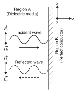
Figure 2-25 Incident electromagnetic wave propagating in dielectric region α and impinging on dielectric region B, showing that a portion of the wave is reflected back in the - z-direction and a portion is transmitted in the +z -direction.

2.7.2 Plane Wave Incident on a Lossless Dielectric
In Section 2.7.1 we considered the special case where a propagating electromagnetic plane wave was incident on a plane boundary where the second medium was a perfect conductor. Now we consider the more general case where the second medium is a lossless dielectric. When a plane wave impinges on an area with a different dielectric, a portion of the wave is reflected and a portion of the wave in transmitted into the new medium, where it continues to propagate, as shown in Figure 2-25.
If we assume that the incident fields are represented by phasors, we can separate the total plane wave into three parts:
1. Incident wave:
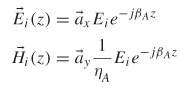
2. Reflected wave:
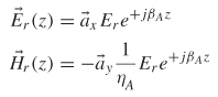
3. Transmitted wave: 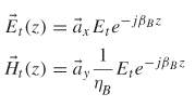
where = ![]() (where μx = μrx μ0 and εx = εrxε0 ) are the phase constants and intrinsic impedances of regions α and B, respectively.
(where μx = μrx μ0 and εx = εrxε0 ) are the phase constants and intrinsic impedances of regions α and B, respectively.
When a wave intersects a boundary between two lossless dielectric regions, the tangential components of both the electric and magnetic fields across the interface must remain continuous. In other words, the tangential component of the fields cannot change instantaneously. In our particular scenario, the plane wave is propagating in TEM mode in the z-direction, so both the electric and magnetic fields are oriented parallel (i.e., tangent) to the boundary of the dielectric interface. Subsequently, we can say that at the interface (z = 0), the sum of the incident and reflected waves must equal the transmitted wave:
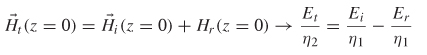
Since the incident waves are known, we can solve (2-128) and (2-129) simultaneously for the transmitted and reflected portions of the wave:
Equations (2-130) and (2-131) lead to the definition of the reflection and transmission coefficients:
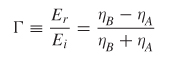

The reflection coefficient is a measure of how much of the wave is reflected back off the intersection between the two media, and the transmission coefficient tells how much of the wave is transmitted. If the reflection coefficient is zero, it means that the intrinsic impedance in the two regions is identical. If the intrinsic impedances are not equal, the reflection coefficient will be finite. Theseequations are used heavily in Chapter 3 when analyzing multiple reflections on transmission-line structures.
REFERENCES
Huray, Paul G., 2009, Foundations of Signal Integrity, Wiley, Hoboken, NJ.
Inan, Umran S., and Aziz S. Inan, 1998, Engineering Electromagnetics, Addison Wesley Longman, Reading, MA.
Jackson, J. D., 1999, Classical Electrodynamics, 3rd ed., Wiley, New York.
Johnk, Carl T. A., 1988, Electromagnetic Theory and Waves, Wiley, New York.
PROBLEMS
2-1 For a TEM plane wave traveling in the z-direction where Ex = 60 V/m, if λ = 20 cm and v = 1.5 × 10⁸, determine the frequency of the wave, the relative dielectric permittivity (εr), the phase constant, and the intrinsic impedance.
2-2 For the wave in Problem 2-1, write formulas for the time-domain expressions for the E and H fields, and plot them.
2-3 For the plane wave in Problem 2-1, how much power is being transported?
2-4 If a wire with a diameter of 1 in. is carrying a dc current of 1000 A, how much power would be delivered to the 100-Ω resistive load in the loop shown in Figure 2-26?
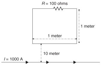
2-5 If two identical point charges are separated by 10 in. in free space and are experiencing a repulsion force of 1 N, what is the magnitude of each charge?
2-6 Assume that two infinitely long parallel wires are separated by a distance of 5 in. with currents that are equal but opposite. Find the current if the force per unit length is 0.25 N/m.
2-7 Determine the energy needed to assemble three point charges in free space from infinity to the following (x,y,z) coordinates: (0,0,0), (1 mm, 0, 0), (-1 mm, 0, 0).
2-8 For a parallel-plate capacitor in free space (εr = 1) with total change Q on one plate and- Q on the other with plate areas of α separated by the distance d, calculate the external force required to keep the plates stationary.
2-9 If a plane wave is propagating in the z-direction in free space and it impinges on a planar dielectric medium where εr = 9.6, how much of the wave is propagated? How much is reflected? If the electric field incident on the boundary has a value of 60 V/m, how much power is carried in the initial wave? How much power is reflected and transmitted? Show that power is conserved.
2-10 If the electric field in an area of space is known to be ![]() =br3
=br3 ![]() r (where b is a constant) in spherical coordinates, find the charge density ρ and the total charge within a sphere of diameter d.
r (where b is a constant) in spherical coordinates, find the charge density ρ and the total charge within a sphere of diameter d.