
Particle S warm Simulation 169
0 1 2 3 4 5
x 10
4
6
8
10
12
14
16
18
Generation
Performance
Asexual
Sexual
Mature Age
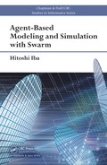
FIGURE 6.28:
Performance comparison.
ten generations. As can be seen in Fig. 6.28, sexual reproduction after the
mature age (800) performs better than asexual reproduction, which is tested
statistically.
In a sec ond experiment, the bacteria in the lower left-hand corner (called
the Garden of Eden, a square of 75 × 75 cells) are replenished at a much
higher rate than normal (Fig. 6.29(a)); the normal ba c terial deposition rate is
roughly 0.5 bac terium per (GA) generation over the who le grid. In the Garden
of Eden, this rate is 0.5 over the 75 ×75 are a, i.e., a rate roughly
512×512
75×75
= 47
times grea ter than normal. As the (GA) g e nerations proceeded, the cruisers
evolved as before. But within the Garden of Eden, the jitterbugs were more
rewarded for their jittering around small areas (see Fig. 6.27). Thus, two kinds
of “species” evolved (i.e., cruisers and twirlers) (Fig. 6.29(c)). Note how typical
gene codes of these two species differed from each other. In this second exper-
iment, three different strategies (asexual reproduction, sexual reproduction,
and sexual reproduction within a reproductive radius) are compared in four
different situations. The aim is to evolve a mix of bugs, namely, the cruis-
ers and twirlers. Two initial conditions are tested: a) randomized initial bugs
and b) cruisers already evolved. In addition, the influence of an e mpty area
in which no bacteria exist is investiga ted. Obviously this empty-area condi-
tion makes the pr oblem easier. T he res ults of these experiments are shown in
Table 6.4.
As shown in the table, sexual reproduction with a reproductive radius
is superior to the other two strategies and the performance improvement is
significant for more difficult tasks such as non-empty-area conditions.

170 Agent-Based Modeling and Simulation with Swarm
(a) (b)
(c)
FIGURE 6.29: Garden of Eden (a) 69th generation (b) 72, 337th generation
(c) 478, 462nd generation.
Therefore, it was confirmed that crossover is useful for the evolution of
predatory behavior. T he method described contrasts with traditional GAs in
two ways: the bugs’ approach uses search directions rather than positio ns,
and selection is based on energy. This idea leads to a bug-based GA search
(BUGS) whose implementation is described in the nex t section.
6.6.2 A bug- based GA search
Those individuals which perform the search in this scheme are called
“bugs.” The function that these bugs maximize is defined as:
f(x
1
, x
2
, ··· , x
n
) wh ere x
i
∈ Dom
i
, (6.26)
where Dom
i
represents the domain of the ith parameter x
i
.

Particle S warm Simulation 171
TABLE 6 .4: Experimental results (sexual vs. asexual selection).
Task Asexual Sexual Sexual
empty mutation crossover Proximity cr ossover
initial area mutation mutation
Random ◦
J
Cruisers ◦
J
Cruisers × △ △
Random × △ △
△ diffi cult ◦ possible fast
J
faster
Each bug in the BUGS program is characterized by 3 parameters:
Bug
i
(t) : po sition
~
X
i
(t) = (x
i
1
(t), ··· , x
i
n
(t)) (6.27)
direction
~
DX
i
(t) = (dx
i
1
(t), ··· , dx
i
n
(t)) (6.28)
energy e
i
(t) (6.29)
where t is the generation count of the bug, x
j
is its jth component of the
search space, and
~
DX
i
is the direction in which the bug moves next. The
updated position is calculated as follows:
~
X
i
(t + 1) =
~
X
i
(t) +
~
DX
i
(t) (6.30)
The fitness of each bug is derived with the aid o f the function (6.26). The
energy e
i
(t) of bug i at time (or generation) t is defined to be the cumulative
sum of the function values over the previous T time steps or generations, i.e.,
e
i
(t) =
T
X
k=0
f(
~
X
i
(t − k)) (6.31)
The format of a bug’s “chromosome” which is used in the BUGS program
is the bug’s real number e d DX vector, i.e., an ordered list of N real numbers.
With the above definitions, the BUGS algorithm can now be introduced:
Step 1 The initial bug population is generated with random values:
P op(0) = {Bug
1
(0), ··· , Bug
N
(0)}
where N is the population size. The generation time is initialized to
t := 1 . The cumulative time period T (called the Bug-GA Period) is set
to a user-specified value.
Step 2 Move each bug us ing eq. (6.30 ) synchronously.
Step 3 The fitness is derived using eq. (6.26) and the ener gy is accumulated
using:
for i := 1 to N do e
i
(t) := e
i
(t − 1) + f
i
(
~
X(t))
172 Agent-Based Modeling and Simulation with Swarm
Step 4 If t is a multiple of T (T -p e riodical), then execute the GA algorithm
(described below) called BUGS-GA(t), and then go to Step 6.
Step 5 P op(t + 1) := P op(t), t := t + 1, and then go to Step 2.
Step 6 for i := 1 to N do e
i
(t) := 0
t := t + 1. Go to Step 2.
In Step 1, initial bugs are generated on conditions that fo r all i and j,
x
i
j
(0) := Random(a, b) (6.32)
dx
i
j
(0) := Random(−|a − b|, |a − b|) (6.33)
e
i
(0) := 0 (6.34 )
where Random(a,b) is a uniform random genera tor between a and b. The
BUGS-GA period T sp e c ifies the frequency of bug reproductions. In general,
as this value becomes smaller, the perfor mance becomes better, but at the
same time, the converg e nce time is increased.
For real-valued function optimization, real- valued GAs are preferred over
string-based GAs (see [58] for details). Therefore, the real-va lued GA approach
is used in BUGS-GA. The BUGS version of the genetic algorithm, BUGS-
GA(t), is as follows (Table 6.5):
Step 1 n := 1.
Step 2 Select two parent bugs Bug
i
(t) and Bug
j
(t) using a probability dis-
tribution over the energies of all bugs in P op(t) so tha t bugs with hig her
energy are selected more frequently.
Step 3 With probability P
cross
, apply the uniform crossover operation to the
~
DX of copies of Bug
i
(t) and Bug
j
(t), forming two offspring Bug
n
(t+1)
and Bug
n+1
(t + 1) in P op(t + 1). Go to Step 5.
Step 4 If Step 3 is skipped, form two offspring Bug
n
(t+1) and Bug
n+1
(t+1)
in P op(t + 1) by making copies of Bug
i
(t) and Bug
j
(t).
Step 5 With probability P
asex
, a pply the mutation operation to the two off-
spring Bug
n
(t + 1) and Bug
n+1
(t + 1), changing each allele in
~
DX with
probability P
mut
.
Step 6 n := n + 2.
Step 7 If n < N then go to Step 2.
The aim of the BUGS-GA subroutine is to acquire bugs’ behavior adap-
tively. T his subroutine works in much the same way as a real-valued GA,
except that it operates on the directional vector (
~
DX), not on the positional

Particle S warm Simulation 173
TABLE 6.5: Flow chart of the reproduction process in BUGS-GA.
Sexual reproduction:
individual energy gene individual energy gene
Parent
1
Bug
i
(t) E
1
G
1
⇒ Parent
′
1
Bug
n
(t + 1) (E
1
/2) G
1
Parent
2
Bug
j
(t) E
2
G
2
⇒ Parent
′
2
Bug
n+1
(t + 1) (E
2
/2) G
2
Child
1
Bug
n+2
(t + 1) (E
1
+ E
2
/4) G
′
1
Child
2
Bug
n+3
(t + 1) (E
1
+ E
2
/4) G
′
2
Reproduction condition ⇒
(E
1
> Reproduction energy threshold) ∧ (E
2
> Reproduction energy threshold)
∧ (distance between Parent
1
and Parent
2
< Reproduction Radius)
Recombination ⇒
G
′
1
, G
′
2
: uniform crossover of G
1
and G
2
with P
cross
, mutated with P
mut
P
asex
?
✟
✟
✟
❍
❍
❍
❍
❍
❍
✟
✟
✟
❄
❄
Yes
✲
No
Return
Asexual reproduction:
individual energy gene individual energy gene
Parent Bug
i
(t) E G ⇒ Child
1
Bug
n
(t + 1) (E/2) G
′
⇒ Child
2
Bug
n+1
(t + 1) (E/2) G
′′
Reproduction condition ⇒ (E > producible energy)
G
′
, G
′′
: mutation of G with P
mut
vector (
~
X). Positions ar e thus untouched by the adaptive process of the GA,
and are changed gradually as a result of increment by eq . (6.30). On the
other ha nd, fitness is evaluated using po sitional potential by eq. (6.26), which
is the same as for a real-valued GA. Furthermore, chromosome selection is
based on cumulative fitness, i.e., energy. The summa ry of differences between
a real-valued GA a nd BUGS is pre sented in Table 6.6.
The main difference lies in the GA target (i.e.,
~
X vs
~
DX) and the selec-
tion criteria (i.e., energy vs. fitness). Remember that the basic idea of this
combination is derive d from a paper [29] w hich simulated how bugs learn to
hunt bacteria (as describe d in Section 6.6.1.1).
Figure 6.30 shows the evolution (over 5 to 53 time steps) of the positions
and directions of the bugs in the BUGS program. These bugs were used to
optimize the following De Jong’s F 2 function (modified to the maximization
problem; see Appendix A.2 for details):
Maximize f (x
1
, x
2
) = −(100(x
2
1
− x
2
)
2
+ (1 − x
1
)
2
)
where −2.047 ≤ x
i
< 2.048. (6.35)
..................Content has been hidden....................
You can't read the all page of ebook, please click here login for view all page.