

Cellular Automata Simulation 189
FIGURE 7.7: Game of life.
As before, implementation by alloca ting one Bug (object) to one cell
can also be done. In this case, update rules are des c ribed in the “step”
method of Bug.java as follows. This can be thought of as an application
of simpleObserverBug2.
public void step(){
int i,j;
int sx, sy;
int num=0;
Bug b;
// Number of live cells around is obtained in ‘‘sum’’
for(i=xPos-1;i<xPos+2;i++){
for(j=yPos-1;j<yPos+2;j++){
if( !(i==xPos && j==yPos) ){
sx = (i+worldXSize)%worldXSize;
sy = (j+worldYSize)%worldYSize;
b = (Bug) world.getObjectAtX$Y(sx, sy);
if( b.isAlive() ) num++;
}
}
}
// Execution of update rules of life and death
if(is_alive){
if(num==2 || num==3){
next_is_alive=true;
}else{
next_is_alive=false;
190 Agent-Based Modeling and Simulation with Swarm
}
}else{
if(num==3){
next_is_alive = true;
}else{
next_is_alive = false;
}
}
}
On the other hand, w riting lattice plane and rules in one class using
“ConwayLife2dImpl” is also pos sible. Let us look at the stepRule method
inside ConwayWorld.java. Here, all coordinates (x, y),
sum += this.getValueAtX$Y(xm1, ym1); // down left
sum += this.getValueAtX$Y(x,ym1); // down
sum += this.getValueAtX$Y(xp1,ym1); // lower right
sum += this.getValueAtX$Y(xm1,y); // left
sum += this.getValueAtX$Y(xp1, y); // right
sum += this.getValueAtX$Y(xm1, yp1); // upper left
sum += this.getValueAtX$Y(x, yp1); // up
sum += this.getValueAtX$Y(xp1, yp1); // upper right
count the number of lives (1) in cells in the eight neighbors. However,
xm1 = (x + xsize - 1) % xsize; // left
xp1 = (x + 1) % xsize; // right
ym1 = (y + ysize - 1) % ysize; // down
yp1 = (y + 1) % ysize; // up
Dividing by xsize, ysize and obtaining the remainder is because it is con-
sidered to be connecting the vertical and horizontal (torus structure) of the
lattice plane. Moreover, the part below calculates the next sta te:
if(this.getValueAtX$Y(x,y)==1) // am I alive (1) ?
newState = (sum==2 || sum==3) ? 1 : 0;
else // if I am dead (0)
newState = (sum==3) ? 1 :0;
Let us try to implement the cellular automaton explained in Section 7.1
by applying Bug (Fig. 7.8). This sample pro gram is a 2 sta te 3 neighbor one-
dimensional automaton, and upda te rules are according to odd parity. In other
words, it takes the majority state in the thr e e cells as the next state. In fact,
a process such as the one given below is performed by laying Bug (object) in
the last line of a two-dimensional FoodSpace grid:
Step1 Bug looks at the state of the bait pla c e d in its neighborhood.
Cellular Automata Simulation 191
FIGURE 7.8 (See Color Insert): One-dimensional cellular automaton.
Step2 This state decides whether the bait sho uld be placed in the next time
or not.
Step3 FoodSpace is shifted one space up.
Step4 Bug place s the food.
Step5 Return to Step1.
Note that to change the rules of state transition, the contents of the method
“step” of Bug.java, which decides the next state, s hould be changed. For
example, it is as follows in the sample program:
public void step(){
int x;
int sx;
int[ ] v = new int [3];
// radius r is 1, therefore, an array of r + 1 + r =3 is prepared
// xPos is its own coordinates
// the three values xPos-1, xPos, xPos+1 are substituted in
v[0], v[1], v[2]
for(x = xPos-1; x < xPos+2; x++){
sx = (x + worldXSize) % worldXSize;
v[x - (xPos-1)] = foodSpace.getValueAtX$Y(sx, yPos);
}
// nextvalue is the next state of xPos
// next state is obtained after checking the parity of v[0], v[1],
v[2]
if( (v[0]+v[1]+v[2])%2 ==1 )
nextvalue = 1;

192 Agent-Based Modeling and Simulation with Swarm
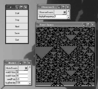
FIGURE 7.9: Execution of Wolfram’s experiment.
else
nextvalue = 0;
}
Furthermore, in or der to increase the states, follow the steps below:
(1) Add the number of colors equal to the number of states you want to use
in colorMap inside ObserverSwarm.java.
(2) Increase the types of bait equal to the number of states you want to use
inside Bug.java.
(3) Modify the state transition rules according ly.
To do the experiment by Wolfram as explained in Section 7.1, let us try to
improve the program. The execution example of the system for that is shown
in Fig. 7.9. Since in this program, the rule number can be entered in "Rule,"
observation of the behavior of vario us classes mentioned above is also possible.
Rule number can also be changed during execution, by the following steps:
(1) If during execution, press the Stop button.
(2) Enter the number to be changed in the "Rule" field. Then press the
Enter key.
(3) Press the "applyRule" button.
(4) If required when you pr e ss the "randomize" button, the cell state is
initialized randomly.
Cellular Automata Simulation 193
(5) Execution starts with new conditions when the "Start" button is pressed.
As the last example, we will explain the self-replicating loop of Langton.
This is a two-dimensional cell automaton with eight states and five neighbors,
and it is something that replicates its own pattern thro ugh 219 transition rules
(refer to Table 7.5). In this chart, the sequence of six numbers represents one
transition rule (in order, state before transition, states of four adjacent cells,
and state after transition). Four cells’ states are considered to be c lockwise,
and may be gin in any direction. For example, in the last rule: 7 0272 0 shows
that the next state o f the center cell, i.e., 7, will be 0 for the following four
cases:
0 2 7 2
272 770 272 077
7 2 0 2
Please note that, in the infinite space, situations not in transition states do
not occur. In fact, since the space is a to rus structure, the occurr e nce of
situations not in the tr ansition rules is possible. However, in that case the
state is updated to 0.
As defined in "initvalue" in FoodSpace.java, the initial state pattern is
a loop as follows:
2 2 2 2 2 2 2 2
2 1 7 0 1 4 0 1 4 2
2 0 2 2 2 2 2 2 0 2
2 7 2 2 1 2
2 1 2 2 1 2
2 0 2 2 1 2
2 7 2 2 1 2
2 1 2 2 2 2 2 2 1 2 2 2 2 2
2 0 7 1 0 7 1 0 7 1 1 1 1 1 2
2 2 2 2 2 2 2 2 2 2 2 2 2
Here, the part without numbers is the part with state 0. How self-replicatio n
goes on through transition o f initial patterns is shown in Fig. 7.10. The rep e -
tition of the extended protruded part bending to the left and the continuation
of the self-replication of the initial state loop can be observed. Cells’ states
loosely mean the following:
• State 0: Background with nothing
• State 1: Tr ansmission passage of signal
• State 2: Tr ansmission passage’s cover e d portion
• State 4 to 7: Transmitted signal
..................Content has been hidden....................
You can't read the all page of ebook, please click here login for view all page.