
184 Agent-Based Modeling and Simulation with Swarm
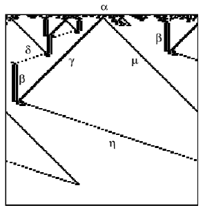
FIGURE 7.3: Explana tion of CA behavior from collision of particles (with
permission of Oxford University Press, Inc. [88]).
γ particles contain information that this is the boundary with a white region,
and a µ particle is a boundary with a white region. When a γ particle collides
with a β particle before colliding with a µ particle, this means that the in-
formation carried by the β and γ particles beco mes integrated, showing that
the initial lar ge white region is smaller tha n the initial large black region that
shares a bo undary. This is coded into the newly generated η particle.
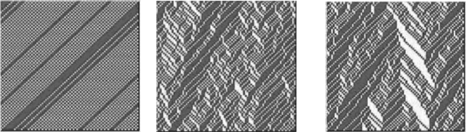
Stephen Wolfram [128] systematically studied the patterns that for m when
different rules (eq. (7.6)) are used. He grouped the patterns generated by one-
dimensional CA into four classes.
Class I All cells become the s ame state and the initial patterns disappear.
For example, all cells become black or all c e lls become white.
Class II The patterns converge into a striped pattern that does not change
or a pattern that periodically repeats.
Class III Aperiodic, chaotic patterns appear.
Class IV Complex behavior is observed, such as disappearing patterns or
aperiodic and periodic patterns.
Examples of these patterns are shown in Fig. 7.4. The following are the rules
behind these patterns (radius 1):
• Class I: Rule 0
• Class II: Rule 245
• Class III: Rule 90
• Class IV: Rule 110

Cellular Automata Simulation 185
(a) Class I (b) C lass II
(c) Class III (d) C lass IV
FIGURE 7.4: Examples of patterns.

186 Agent-Based Modeling and Simulation with Swarm
TABLE 7.4: Rule 184.
a
i−1
t
, a
i
t
, a
i+1
t
111 110 101 100 011 010 001 000
a
i
t+1
1 0 1 1 1 0 0 0
Here, transition rules are expressed in 2
2
3
bits from 000 to 111, and the number
of the rule is the decimal e quivalent of those bits. For instance, the trans itio n
rules for Rule 110 in Class IV are as follows [83]:
01101110
binary
= 2 + 2
2
+ 2
3
+ 2
5
+ 2
6
= 110
decimal
(7.9)
In other words, 000, 100, and 1 11 be c ome 0, and 001, 010, 011, 101, and 110
become 1.
Rule 110 has the following interesting characteristics in co mputer science.
(1) Is computationally universal [128].
(2) Shows 1 /f fluctuation [91].
(3) Prediction is P-complete [90].
Kauffman proposed the concept of the “edge of chaos” from the behavior of
CA as discussed above [67]. This concept represents Cla ss IV patterns where
periodic patterns and aperiodic, chaotic patterns are repeated. The working
hypothesis in artificial life is “life on the edge of chaos.”
7.1.1 Rule 18 4
Rule 184 is k nown as the Burgers cell auto maton (BCA), and has the
following important characteristics (Table 7.4).
(1) The number of 1s is conse rved.
(2) Complex changes in the 0-1 patterns are initially observed; however, a
pattern always converg e s to a right-shifting or left-shifting pattern.
Take a
i
t
as the number of cars on lattice point i at time t. The number
is 1 (car e xists) or 0 (no car exists). The car on lattice point i moves to the
right when the lattice po int is unoccupied, and stays on the lattice point when
occupied at the next time step. This interpretation allows a simple description
of traffic congestio n using rule 184.
BCA can be e xpanded as fo llows:
• BCA with signa ls: restrict traffic to the right at each lattice point
• Probabilistic BC A: move with a probability
Cellular Automata Simulation 187
(a) α = 1.0, no signal (b) α = 0.8, no signal (c) α = 0.8, signal type 110
FIGURE 7.5: Congestion simulation using BCA.
An in-depth explanation of CAs describing traffic congestio n is given in section
7.9.
Figure 7.5 shows a result of BCA simulation. Cars are shown in black
in this simulator. Continuous black areas represent congestion because cars
cannot move fo rward. Congestion is more likely to form when the probability
that a car moves forward α is small. Figure 7.5(a) shows how congestion forms
(black bands wider than two lattice points form where a car leaves the front
of the congestion and another car joins at the rear). A signal is added at the
center in Figure 7.5(c). The signal pattern is shown in blue when 1 and red
when 0, and the pattern in this simulation was 110 (i.e., blue, blue, red, blue,
blue, red,. . .).
The Swarm simulator using BCA is an applicatio n of one-dimensional CA,
and the par ameter probe in ObserverSwarm displays the fo llowing parameters.
• worldSizeX: size of the spac e (horizontal a xis)
• worldSizeY: size of the spac e (vertical axis)
• Alpha: pro bability that a ca r moves to the right
• Signal1: pattern of signal 1
• Signal2: pattern of signal 2
The proba bility that cars move to the right and the pattern of signals can
be changed during runs by clicking the “Stop” button, changing values, and
re-running. Here, after changing the parameters, you need to press “Enter”
and click the applyRule button.
A s imulation of silicon traffic based on these models is shown in Fig. 7.6.
A two-dimensional map is randomly generated, and cars are also placed at
random. Two points are randomly chosen from the nodes on the map and
are designated as the or igin and the des tina tion. The path from the orig in to
the destination is determined by Dijkstra’s algorithm. Here, a co st calculation
where the distances between nodes are we ighted with the density of cars in
each edge is performed to determine a path that avoids congestion. The signal

188 Agent-Based Modeling and Simulation with Swarm
FIGURE 7.6 (See Color Insert): Simulation of silicon traffic.
patterns are designed to change the passable edge in a given order at a constant
time interval.
7.2 Conway class with Swarm
A standard class to describe cellular automaton is
Class ConwayLife2dImpl
The advantages of using the Conway class are
(1) The des c ription of a cell automaton is easy.
(2) Faster execution of update rules is possible.
For example, let us ma ke a life game program (Fig. 7.7). You might guess that
in this game cells are spread all over the square lattice, and either take up life
(1, on) or death (0, off). The state of cells is updated by the following rules:
(1) If the s tate of cells is death, it comes back to life next time if out of the
eight surrounding places three are alive.
(2) If the state of cells is life, it stays alive next time if out of the eig ht
surrounding places two or three are alive. Else, it dies in the next time.
..................Content has been hidden....................
You can't read the all page of ebook, please click here login for view all page.