
214 Agent-Based Modeling and Simulation with Swarm
+getPercolationProb()
+showStats()
+showHist()
+checkT
oStop()
+graphInterval
-colorMap
-displayActions
-displaySchedule
-statActions
-statSchedule
ObserverSwarm
+checkToStop()
+getPattern()
+width
+height
ModelSwarm
+remainingQ()
+update()
+trace()
-traceCluster()
+getClusterNum()
+getClusterSizeData()
+getP
ercolationProb()
-largestCluster
-remainingPoints
-clusterData
-clusterSizeData
PatternSpace
1 1 1 1
+step()
EZGraph
+reset()
+update()
+output()
EZBin
1
1
1
1
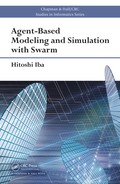
FIGURE 7.22:
The whole structure for percolation.
FIGURE 7.23: patternSpace: the dar k portion is the largest cluster.
FIGURE 7.24: Percolation probability.

Cellular Automata Simulation 215
FIGURE 7.25: Histograms in Swarm.
(2) Setting of title
(3) Setting of collection
(4) Setting of “selector” of probe
(5) Setting of number of “bin”
(6) Setting of upper and lowe r limits of display
7.9 Silicon traffic and its control
The following is an explanation of traffic modeling. Nagel and Shreckenberg
modeled traffic congestion using a one-dimensional CA [89]. In their model,
each cell corresponds to a position where cars can pass, and each cell can take
one of two states (one or no car is in the cell) in every time step. Every car
moves at a characteristic speed (integer value from 0 to v
max
). The speed of
the cars and the state of the cells are updated based on the following rules.
Acceleration Incr e ase the speed by one unit (v := v + 1) if the speed of a car
v is less than v
max
and the distance fro m the first car ahead is greater
than v + 1.
Deceleration Decrease the s peed of a c ar at i to j −1 (v = j −1) if the firs t
car ahead is located at i + j and j ≤ v.
Random number Decrease the speed of all cars by 1 (if larger than 0) at
possibility p (v := v − 1).
Move Move all cars at their res pective speed v.

216 Agent-Based Modeling and Simulation with Swarm
time
space (road)
FIGURE 7.26: An example of the flow of c ars.
The most important parameter in this simulation is the density of car s ρ,
defined as
ρ =
total number of cars
total number of cells
(7.14)
Figure 7.26 is an example of the flow of cars w ith v
max
= 5 and ρ = 0.1. Cars
move from left to right, and the right end is connected to the left end. The
numbers indicate the speed of the cars, and the dots show cells with no cars.
Consecutive cars at s peed 0 at the center indicate traffic congestion.
Nagel and Shr e ckenberg conducted various experiments and found that the
nature of conge stion changes at ρ = 0.08. Note that congestion is measure d by
the ave rage speed of all cars. Thus, the critical value for this traffic simulation
is ρ = 0.08.
7.9.1 Simulating traffic jams with Swarm
Nagels and Shrecke nberg performed the modeling o f traffic jams using a
one-dimensional lattice. In their model, e ach cell corresponds to the vehicle’s
passage, at each time-step, and the cells take one of the two states (vacant or

Cellular Automata Simulation 217
FIGURE 7.27 (See Color Insert): Simulating a traffic jam (with Slow-
toStart).
occupied by one vehicle). All the vehicles move with a specific speed (integer
number, 0 to v
max
). This model was visualized and implemented on Swarm.
To see the time change of one-dimensional cellular automaton (CA), it is
drawn on PatternSpace (Discrete2d). To implement a two-dimensional CA
like the life ga me, it is good to use DblBuffer2d, which has two buffers. For
example, the movement of a car with v
max
= 1 0, ρ = 0.1 is shown in Fig. 7.27.
The vehicle moves in the right-hand direction, and the right end a nd the left
end are connected. The top row shows the current ro ad conditions, and the
time passe d as we move down (displayed for 200 steps). In Swarm, the vehicles’
sp e e d is represented by shades of color s. In fact, green becomes dar ker with the
increase in speed, and the red beco mes darker as the speed decreases (as set
in colorMap). A chunk of red color is the point of occur rence of a traffic jam,
and the black part shows a cell without a vehicle. In Fig. 7.27, the occurrence
of a series of vehicles with sp e e d 0 in the middle is a traffic jam. We can see
that the traffic jam moves forward with time.
In this model, SlowtoStart has been introduced to realize the effect of
inertia. This is a rule that says once the vehicle has sto pped, it starts moving
after 1 time s tep even if the front is open to move. This is considered impor tant
to bring the model closer to actual metastability. If SlowtoStart is used, it takes
time to accelerate, which leads to more stationary vehicles and worsens the
traffic jam (Fig. 7.27). On the other hand, without SlowtoStart, the line of
the stationary vehicles w ill not elongate unless there is a slowdown due to a
random number, and therefore as a result, the traffic jam is eased (Fig. 7.28).
Recently ASEP (Asymmetric Simple Exclusion Process) has been studied
extensively as a model of traffic flow [99]. In this model, the maximum speed
of each vehicle existing in each cell is taken as 1; if the c e ll in front is vaca nt,
the vehicle moves to it with a probability p (stops with a probability 1 − p).
Let us take the inflow and outflow probabilities of new cars as α and β,
respectively (in other words, right and left ends are not connected, and the
number of vehicles is not fixed). Figure 7.29 shows the ASEP model simulation
in Swarm. Parameters are α = 0.3, β = 0.9, p = 0.5 for (a) free phase, α = 0.3,

218 Agent-Based Modeling and Simulation with Swarm
FIGURE 7.28 (See Color Insert): Simulating a traffic jam (without Slow-
toStart).
(a) free phase (b) shockwave phase (c) maximum flow phase
FIGURE 7.29: ASEP model simulation.
β = 0.3, p = 0.5 for (b) shockwave phase, and α = 0.6, β = 0.6, p = 0.5 for
(c) maximum flow phase. In this case, colorMap is set such tha t black p oints
show cells with vehicles, and the white part shows vacant cells. As explained
earlier, the topmost row is the current road s itua tion. As we go down, it shows
the time already passed. In the ASEP model, various mathematical analyses
are done for the equilibrium state [99].
7.10 The world of Sugarscape
In this section, we discuss Sugarscape models and their simulation. Sug-
arscape was presented by Joshua M. Epstein and Robert Axtell as an ex-
perimental model environment for creating artificial societies. Sugarscape is
based on the simulation of an unlimited number of ants walking around in
search of sugar. The model can construct artificial societies with the aim of
examining the mechanisms driving various social phenomena, and allows the
..................Content has been hidden....................
You can't read the all page of ebook, please click here login for view all page.