Extensions
THE 14 EXTENSIONS developed here are as follows:
1. Endogenous destructive radius
2. Age and impulse control
3. Flight rather than fight
4. Replication of the Latané-Darley experiment
5. Introduction of memory
6. Coupling of affect and cognition
7. Endogenous changes in weight strength through affective homophily
8. Growing the Arab Spring
9. Jury processes
10. Emergent dynamics of network structure
11. Vertical structure and multiple scales
12. The 18th Brumaire of Agent_Zero
13. Introduction of prices and seasonal economic cycles
14. Endogenous mutual escalation spirals
III.1. ENDOGENOUS DESTRUCTIVE RADIUS
Just as agents can differ in their search radii, so they may differ in their destructive radii. Thus far, this has been treated as a single exogenous global constant. It is more realistic—and reduces the number of freely adjustable parameters—to endogenize this action radius. It might, for example, be a function of affect, or of total disposition.152 In Figure 48, the destructive radius is a simple linear function of disposition and thus differs among agents (and varies in time). This is a fertile extension, especially in the various alternative interpretations of the framework.

FIGURE 48. Endogenous Action Radii
Health Interpretations
For example, where the action is vaccine refusal—itself an area rife with emotional contagion153—some agents foreswear all vaccines within a large pharmaceutical radius, while others refuse only a narrow set (a small radius). In an eating interpretation, some indulge in bingeing across many food groups, while others confine themselves to one. In the obesity interpretation, for example, a large binge radius may be the result of a specific deficiency in dopamine receptor availability.154
Now interpret yellow patches as healthy financial assets, and neighboring yellow patches as “similar” ones (stocks in the same industry, for example). Assets turn orange when they suddenly lose value. The destructive radius is the set of assets dumped in response. This can certainly grow with fear and contribute to cascading crises through contagion. In Figure 48, the rightmost agent’s affect is quite low and his destructive radius is confined to one orange site. But the upper left agent’s fear is high, so in response to a single orange devaluation, he dumps a large radius, including healthy yellow assets.
III.2. AGE AND IMPULSE CONTROL
Large action radii might well be interpreted as evidence of poor impulse control or some specific deficiency in executive function. For example, in distinguishing between minors and adults, the U.S. legal system recognizes a difference in juvenile and adult impulse control. The psychology literature surrounding impulse control over the life course is large but reinforces the general pattern: the younger you are, the worse your impulse control (Mischel et al., 2011). Thus far, agents have not advanced in age. So, here we’ll do a double extension: we’ll have them age, but we’ll also have impulse control increase with age. We will think of impulse control as the gap between one’s affect and one’s destruction. For agents with poor control, the damage is far out of proportion to affect, while mature agents can align the two. Specifically, let us posit that when one is born (age zero), impulse control is nil, and one’s damage radius exceeds one’s affect by a factor k > 0. If this impulsive excess is assumed to shrink linearly with age, we arrive at the following functional form:
![]()
NetLogo Code for aging and for this function are provided in the relevant Applet. But, the younger you are, the more your damage exceeds your affect (i.e., the worse your impulse control). The two approach equality as agents approach the maximum age. Figure 49 gives a simple example. All three agents are stationary in the active quadrant, and so are getting comparable stimuli. The upper agent goes first at age 8. The lower agent goes second at age 22, and the third goes at age 36. Their radii are successively smaller, reflecting their increased impulse control with age.155

FIGURE 49. Age and Impulse Control
Obviously, a wide variety of other effects of age can be modeled. Indeed, impulse control itself might be unimodal, declining again with age (e.g., with dementia). Beyond cognitive effects, loss of visual acuity (e.g., contrast sensitivity)156 could be directly represented as a reduction in the spatial sampling radius, while decline in aerobic capacity157 could be represented as a reduction in the distance traveled per step. The general loss of mobility with age obviously affects the elderly’s ability to evacuate in disasters or migrate from politically or environmentally hostile areas, which brings us to the topic of flight in general.
In the exposition thus far, agents have responded to aversive stimuli with direct action on a neighborhood of sites. Destruction—a “fight” response—has been our prime example. Another possible response, of course, is flight. A reasonably general model should permit both fight and flight. The latter is easily arranged in our framework. In fact, the NetLogo Applet provided on the Princeton University Press Website offers users a simple switch. If it’s in the “on” position, agents fight (destroying aversive patches). If it’s in the “off ” position, they flee aversive stimuli. A direct comparison of fight and flight cases—where everything else is the same—is quite interesting.
Beginning with the fight case, for illustrative purposes, we will increase the retaliatory damage radius to 2 in each N, S, E, and W direction so that 12 sites are taken out. With agents in fixed positions (since we are contrasting to flight), a representative run is depicted in Figure 50.
Movie 5 shows that for the arbitrary settings (see the Parameter Table, Appendix IV) employed, the agents fight (retaliate on yellow sites) in a certain order: the southern agent goes first, then the western, and then the eastern. The last is moved to do so through the weighted (solo) dispositions of the first two.

FIGURE 50. Fight [Movie 5]
This is also the same sequence in which the agents begin to flee, as shown in the four snapshots of Figure 51.
I highly recommend the movie version, Movie 6 on the book’s Princeton University Press Website, because it clearly shows the upper-right agent being “dragged” out by the other two. This is the analogue of them “convincing” him, through their weights, to finally act as they have.
So, here are two runs in which the only change is flight versus fight. Everything else is identical, including the random seed and all the stochastic activations generated. Suppose we now ask the question: How, if at all, do the disposition trajectories differ in these two (fight vs. flight) runs? And, if they differ, why?

FIGURE 51. Flight [Movie 6]

FIGURE 52. Fight vs. Flight Dispositions Compared
They differ radically, as shown in Figure 52. Under fight (left), net disposition exceeds zero briefly but then remains low throughout. Under flight, it grows dramatically, settling down to sustained levels only when agents are clear of the entire stimulus area. Why are they so different? Because the stationary fighters eliminate the stimulus and never move into new active areas. The refugees, by contrast, cross the entire field of active stimuli as they evacuate, as it were, continuously increasing their affect, their probability, and the weighted sum of their colleagues’ values, all of which is aggregated to form their disposition. If evacuation subjects the refugee to a relentless field of adverse stimuli, shelter-in-place may be the less traumatic course—if it is feasible.
An area where the dilemma of shelter-in-place vs. evacuate arises very sharply is in chemical, biological, and radiological contamination scenarios (Fischhoff, 2005). Obviously, evacuation through a contaminated zone might be riskier than staying put. But if the contaminant is purely airborne, then depending on the wind field, the fluid dynamics, and available transport capacity, evacuation might dominate. For an urban-scale simulation combining computational fluid dynamics and agent-based modeling, see J. M. Epstein, Pankajakshan, and Hammond (2011). Mainly, it is clear that the areas of refugee behavior and crisis evacuation could be studied in this framework.
We will return to the topic of flight when we replicate the famous Latané-Darley experiment. There, the orange patches represent smoke, and—unlike the preceding example—once a patch turns orange, it stays orange; the smoke does not dissipate but eventually fills the room.
Such situations also occur in economics. Some assets (e.g., houses) can lose value and never recover. So, imagine agents as investors, each of whose “portfolios” is the set of all patches within their financial vision. Yellow patches have high value. If a patch turns orange, it suddenly loses value—and does so permanently. As the market collapses, investors migrate their portfolios from low-value patches to high-value ones. We see capital flight, in other words, as agents (located at the center of their portfolio) migrate in the southwesterly direction in asset space. Interagent weights capture contagion effects, and the most financially fretful can, just as before, “pull” other agents into financial flight. See Figure 53.
With no recovery of value (no reversion to yellow), the agents encounter even more aversive stimuli along their path. Consequently, everyone’s affective, probability, and disposition curves—all amplified by contagion—are even higher than before. Net disposition to flee one’s portfolio, shown in Figure 54, contrasts with the preceding two examples.
Physical flight figures centrally in one of Latané and Darley’s classic experiments in social psychology. A small extension of the basic model will permit us to replicate this in the Agent_Zero framework.
III.4. REPLICATING THE LATANÉ-DARLEY EXPERIMENT
Much empirical work with agent-based models (including my own) aims to replicate large systems, such as infectious disease dynamics, stock-market dynamics, or distributions of firm sizes, city sizes, and the like. So, it is natural to question whether a three-agent model could hold the slightest empirical interest. It happens that many of the most famous experiments in social psychology involve only three people. Two of these are the Milgram (1963) experiment and Latané and Darley’s 1968 experiment. We will “replicate” the latter of these. That is to say, we will see if Agent_Zero can behave essentially as humans behaved in this experimental setting.
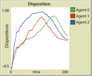
FIGURE 54. Disposition to Flee Portfolio
The Latané-Darley experiment is very clear. It compares behavior in the absence of others to behavior in the presence of others. In the first case, the subject is seated alone in a room. Smoke begins to enter the room. He becomes agitated, eventually afraid, and when his affect and risk appraisal exceed some level, he exits the room and reports the smoke. In the second preparation, the subject is seated in the room with two strangers (who, unbeknownst to the subject, are confederates of the experimenter). Smoke enters the room, just as before. The confederates take no notice whatever and continue filling out forms. In this case the subject takes much longer to exit the room and report. So, the same physical environment stimulates different behavior. Can we generate that in our simple agent model? With one very simple extension, we can.
Without loss of generality, the skeletal equation for two agents posits that Agent 1’s net disposition (subtracting the threshold) is given by
![]()
Since Agent 2 is a confederate and knows the smoke to be a ruse, his V and P are both zero and, in the model, should have no effect on Agent 1. Agent 2’s own threshold does not figure in Agent 1’s disposition, as has been assumed throughout. We appear to be at a loss for any mechanism that would alter Agent 1’s behavior. Suppose, however, that Agent 1 were to impute some threshold to Agent 2 and incorporate it in equation [39]. Denote this imputed threshold as ψ12.158 Then the ![]() equation becomes
equation becomes
![]()
With three agents, if we assume ψ12, ψ13 > 0, we generate the qualitative result of interest.
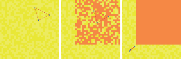
Using ψ12 = ψ13 = 1.5, Figure 55 offers two snapshots of the experiment recorded by hidden ceiling cameras (as it were) looking down on events. The orange patches are smoke filling the room.
The solo agent of Figure 55 exits after around 25 time intervals, while in the trio treatment (right panel), he takes three times as long. These screen shots were taken just as the subject exits the room. Notice that there is less smoke on the left than on the right. Complete movies of the solo and trio cases are given as Movies 7 and 8 on the book’s Princeton University Press Website.159
So, in a very simple sense, we have replicated Darley and Latané’s basic qualitative result: Subjects behave differently in the two cases, and we have the same direction of change as they observed.
Now, why is this happening? Since they know the smoke to be a ruse, the confederates’ affect (their Vs) and their appraisals of risk (their Ps) are both zero. So, how are they influencing the subject’s behavior at all? What mechanism, in the model (as against the brain), is producing the different behavior in the two cases? Threshold imputation is the mechanism.
Without loss of generality, assume Agent 1 to be the subject. For him to flee the room when alone, all we require (suppressing time) is that V1+P1>τ1. But imputing thresholds to others, his disposition becomes
![]()
For the confederates, V2 = P2 = V3 = P3 = 0, leaving

FIGURE 55. Solo vs. Trio Latané-Darley [Movies 7 and 8]
![]()
For ![]() to be positive in this case, we require not merely that V1 + P > τ1 but that V1 + P1 > τ1 + ω21ψ12 + ω31ψ13. This is a higher threshold as long as ψ12 and ψ13 are positive and, accordingly, it takes longer to exceed it!160 This is plausible. First, simply as fellow humans, they have some, perhaps tiny, weight on the subject agent (indeed it suffices for only one of their weights to be positive). Second, even though they are confederates, there is some level of danger that would stimulate them to act, or at least, so thinks any normal Agent 1. So, as long as he imputes even the smallest threshold to them, his overall threshold will rise in their presence. In fact, he will more likely impute high thresholds to them, making for the dramatic difference we see! Here, then, is a simple generative mechanism for bystander effects.
to be positive in this case, we require not merely that V1 + P > τ1 but that V1 + P1 > τ1 + ω21ψ12 + ω31ψ13. This is a higher threshold as long as ψ12 and ψ13 are positive and, accordingly, it takes longer to exceed it!160 This is plausible. First, simply as fellow humans, they have some, perhaps tiny, weight on the subject agent (indeed it suffices for only one of their weights to be positive). Second, even though they are confederates, there is some level of danger that would stimulate them to act, or at least, so thinks any normal Agent 1. So, as long as he imputes even the smallest threshold to them, his overall threshold will rise in their presence. In fact, he will more likely impute high thresholds to them, making for the dramatic difference we see! Here, then, is a simple generative mechanism for bystander effects.
Notice that threshold imputation retrodicts that a single confederate, rather than Darley and Litane’s original two, can suffice to delay the subject’s exit,161 which they also found (Latané and Darley, 1968). Ceteris paribus, we would further retrodict that the effect would be weaker in the single confederate case—the subject should leave later than when alone, but earlier than when there are two confederates. This, too, was found.
Notice that no specific functional forms for the deliberative or affective components (e.g., the Rescorla-Wagner equations) entered into this discussion. We thus see that the skeletal equations alone, the full differential equations, and the agent-based model are all illuminating, as is the dialogue among them.
On the affective side, agents can show inertia. When trials (attacks) cease, the strength of their association between the indigenous population and violence can fall at some rate, the extinction rate. If this rate is low, then there is substantial persistence of affect. By contrast, in estimating probabilities, the agents developed thus far have no memory, or inertia, whatsoever. At every iteration, they use only the current relative frequency of orange (to total) agents within their “vision” to estimate the attack probability.
This seems somewhat implausible for humans. If the attack (i.e., adverse event) rate has been consistently high for the last 10 days, the mere fact that it is zero today may not lead us to forget the entire history and assume a rate of zero for tomorrow. We certainly might reduce the expectation of attack, but the history casts some shadow on projections of the immediate future. Exactly how it does so is a vastly complex matter and depends on the history and the type of memory.
Since I am conceptualizing this as part of Agent_Zero’s deliberative, empirical, data-based, component, it would fall under what neuroscientists call declarative memory capacity. And since it involves a sequence of discrete aversive occurrences, it would engage what is termed episodic memory.162 Episodic memory undoubtedly involves a widely distributed network of brain systems. But the hippocampus and parahippocampus are centrally implicated in this capacity. The latter is hypothesized to play the greater role in the immediate updating of the event history, which is stored more generally in working memory controlled by hippocampus (Eichenbaum, 2000; Smith and DeCoster, 2000). On neural mechanisms of memory, see Kandel (2001).
As emphasized throughout, I am not modeling these (or any other) brain regions. My aim is to offer a simple plausible model of performance, shaped by our evolving knowledge of process and by the broader empirical literature. For these purposes, many mathematical—signal processing—strategies present themselves. In selecting one, let us begin by recalling the kind of signal Agent_Zero gets from his stochastically aversive environment over, for instance, 100 periods.

FIGURE 56. Fixed Agents in Stimulus Field
Figure 56 gives a typical snapshot of the agents. Agents 1 and 2 are in the hostile northeast quadrant of our space. The attack rate is 50.
Each period they “calculate” the relative frequency of orange outbursts within their vision (here vision = 4). Their resulting frequency time series are shown in Figure 57.
There are two things to notice, one individual, and one social. First, the signals for Blue and for Red are highly variable.163 And, depending on action thresholds, this might produce equally variable action dispositions and wildly erratic behavior, whipsawed by environmental variability. This happens, but one’s model should at least permit the representation of less-jittery behavior. The second thing to notice is social: with memory zero in a spatially stochastic environment, the (spatially proximate) agents, in addition to being volatile, are only weakly correlated. Presented with signals of the sort plotted in Figure 57, the range of methods for extracting underlying regularities is vast, from Fourier analysis to extract periodicities, as conducted unconsciously by our Organ of Corti (Wagenaar, 1996) to wavelets and neural networks (Akay, Akay, and Welkowitz, 1994). However, the simplest filter used on high-volatility data is the moving average. Here, one uses the average of the most recent m readings, where m is the memory, also called the sampling window or reading frame. So, if m = 10, one uses the most recent ten observations. Every time step (e.g., day), the most recent is added, and the least recent is dropped.164

FIGURE 57. Unprocessed Frequency Signal
Before, the agent used simply his estimate of relative frequency within the spatial sampling radius (v) at each time, RFv(t). Using the moving average over the preceding m periods, his probability estimate becomes
![]()
which obviously reduces to the previous case for m = 1 (i.e., processing only the current period). This produces smoother dynamics for each individual and (for our neighbors) greater consensus among them, as shown in Figure 58, for a memory window, or “reading frame,” of 25 periods (all other parameters are as in Figure 57).
Neighboring agents standing in a turbulent bathtub will experience very different signals on short time scales. But over a large window, their average signals will be more closely correlated.

FIGURE 58. Moving Average (25)
Limits of the Moving Average
Numerous refinements are possible. For one, in a moving average each memory receives equal weight, when memory can decay with time, an effect often handled with linear or exponential weighting.165 More interesting cognitively, there can also be powerful anchoring effects (Tversky and Kahneman, 1974). My favorite of their demonstrations works as follows: Different subjects are read a string of numbers and asked to estimate their product. When a series of integers is presented from highest to lowest, their product is systematically estimated as far larger than when the same sequence is presented from lowest to highest. That is, if numbers are read aloud in the order 8 × 7 × 6 × 5 × 4 × 3 × 2 × 1, the product is systematically estimated as being far larger than if the numbers are announced as 1 × 2 × 3 × 4 × 5 × 6 × 7 × 8. We “anchor” on the first number we hear—the 8 vs. the 1 (Tversky and Kahneman, 1974, p. 1128). The moving average is insensitive to presentation order. One could capture anchoring by assigning a maximum weight to the first item presented and then having weights successively decline as successive items are presented. The recency effect (e.g., Deese and Kaufman, 1957) would be just the reverse, with maximum weight always shifted to the most recent item presented.
Moving Median
Another simple way to confer stability on the agent’s remembered distribution of sample estimates is to use the moving median rather than the moving average. Of course, the moving median ignores outliers—such as new extreme evidence. It is thus less vulnerable to anchoring. In some cases, this is realistic, as when people fanatically stick to their opinions despite new counterevidence. Sometimes, however, we do the opposite, giving undue weight to extreme events. And, of course, people may differ as well in the length of their memory and in their processing of it.
The NetLogo Code allows the user to choose any memory window and either the moving average or moving median. We will use the moving average in a number of extensions that follow, perhaps most colorfully in extension XII, The 18th Brumaire of Agent_Zero. But we turn now to a set of couplings between components of Agent_Zero.
III.6. COUPLINGS: ENTANGLEMENT OF PASSION AND REASON
Thus far, I have modeled the affective, deliberative, and social components as independent; they all affect disposition, but none depends on—is an explicit mathematical function of—the others. They are decoupled. But, in fact, we have considerable evidence that they are entangled. Here I explore some simple ways of modeling the influence of affective dynamics on (a) probability estimates and (b) network structures. These extensions, neither of which increases the number of freely adjustable parameters in Agent_Zero, are as follows:
1. Probability estimate is influenced by affect.
2. Interagent network weights vary with affective strength and homophily.
Emotional Amplification of Probability Estimates
Throughout, I have modeled Agent_Zero’s probability estimates as being independent of his own affect. To be sure, the probability estimates have been biased. But it has been a sample selection bias. Affect, per se, has not been a source of bias. One of the more interesting and well-established things about humans is that our emotions do bias our estimates of relative frequency—and do so in a systematic direction. In general, this phenomenon falls under what Paul Slovic termed the affect heuristic (Slovic et al., 2007; Kahneman, 2011). More recently, Lerner, Gonzales, Small, and Fischhoff (2003) found that “In a nationally representative sample of Americans (N = 973, ages 13–88), fear increased [terrorist] risk estimates. …”
So, what is the simplest way to extend the model to permit this? Mathematically, we require that the higher the emotion (e.g., fear), the greater the upward bias. However, if the emotionally neutral probability estimate is already 1.0, there is no possible increase, whereas if the initial estimate is close to zero, the room for upward bias is great. If affect is at its absolute maximum, let’s assume that probability is estimated at 1.0, although lower upper bounds are plausible.
In addition to these functional desiderata, let’s also avoid introducing any new variable into the model. One simple way to do all this is as follows: If Pn is the emotionally neutral estimate (which may still be biased statistically), then the emotionally affected estimate, Pe is given by
![]()
When V is zero, there is no emotional bias and Pe = Pn. When V is 1, there is maximum emotional bias and Pe = 1.
This works nicely, as the plots in Figure 59 suggest. The y-intercept is the initial estimate of P and always ranges from 0 to 1; we show different plots for different Pn values. The greatest impact of emotional bias occurs where the Pn is lowest. This accords with the experimental results of DeSteno, Petty, Wegener, and Rucker (2000).
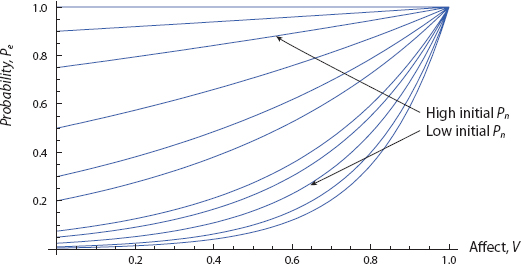
FIGURE 59. Probability Estimate as Function of Affect
We will introduce this variation into the agent model shortly. But, just to keep the agent-based model honest, as it were, we will first incorporate it into the mathematical version. Recall the skeletal equation166
![]()
Here, affect (V) has no effect on probability judgment (P). If we now introduce the preceding affect-dependent variation, we obtain
![]()
Now we can ask, What is the effect of Agent j’s affect on Agent i’s total disposition? This is the cross-partial derivative, ![]() .
.
![]()
But the limiting value of this cross-partial, as Vj approaches zero, is
![]()
This is quite intriguing. If weight is unity, then, as affect is dialed down, the impact of j’s affect on i’s disposition approaches 1 plus the binary entropy of j’s probability distribution. If j is certain, this entropy is zero and the partial is just ωji as in [45].167 But otherwise, j’s estimate affects i’s disposition in an information-theoretic way. Again, this result is independent of the specific functional forms chosen for V and P.
Political Corollary
Observe also that entropy, −p ln p, is hump-shaped (unimodal) with minima of zero at p = 0 and p = 1. So, to maximize her marginal effect on i’s disposition, j should, in fact be “evenhanded,” expressing a probability estimate of 0.5. If politicians knew this theorem, political debate might be far less polarized.

FIGURE 60. Stationary Agent in Stimulus Field
Equation [48] is, as noted, a limiting case. But, precisely such an asymptotic connection to entropy would be hard to notice from agent simulations alone, and serves once more to illustrate the usefulness of having mathematical and computational versions “talk to one another.”
Now let us return to our agent, situated in a spatial field with aversive stimuli, as shown in Figure 60.
We immobilize our subject and bombard her with aversive orange stimuli. With no affective influence, her increasing fear has no effect on her estimate of orange relative frequency (probability), as shown in Figure 61.
However, if affect/emotion influences probability judgment as specified in equation [44], then probability escalates under the identical affective trajectory,168 as is shown in Figure 62.

FIGURE 61. No Affective Amplification

FIGURE 62. Affective Amplification
Mutual Amplification
The individual’s dispositional dynamics (since it varies as the sum of affect and probability) will be amplified accordingly, as will the agent’s level of action, be it retaliatory violence, pandemic flight, or financial panic. Under this kind of emotional amplification, the network of coupled agents can easily work itself into a mutually reinforcing dispositional frenzy, with precious little hard empirical evidence, as illustrated by the low initial P curves of Figure 59. Again, this is far from canonically rational behavior, but is well within the behavioral compass of Agent_Zero society.
Zillmann’s Experiment Revisited
We discussed the general interaction of emotional arousal and cognitive/evidentiary inhibitors of retaliation earlier in connection with the experiment of Zillmann et al. (1975). Zillmann does not propose a mathematical relation. But the one we’ve introduced is broadly consistent with the pattern he observed. Specifically, in our development thus far, we have been interpreting P as the empirical component of our disposition to act. Hence, we can interpret (1 − P) as the mitigating evidence against action. Previously, we postulated that the P-value is amplified by emotional arousal (e.g., fear) as
![]()
But then the mitigating evidence, 1 − P, is damped accordingly: as the level of arousal (V) increases, the weight placed on mitigating evidence (1 − P1 – V) decreases. In the limit of maximum V, it is ignored entirely, since in that V = 1 case, we have
![]()
as per Zillmann et al. (1975). Here, then, is a candidate mechanism that could, in principle, be tested in a laboratory.
Group Implication
Turning as always to the group implication, we observe that if everyone is subject to affective amplification as before and their dispositions are strongly coupled (high weights), then extremely explosive dispositional dynamics can arise from stimuli that would not suffice to trigger any individual’s isolated action.
Agent_Zero Does Jury Duty
This problem is recognized in the rules of evidence in jury trials. It is understood that emotionality—high V produced by inflammatory evidence—can bias a juror’s estimate of the guilty probability (Pe). Moreover, the present model would suggest that with sufficient weight, the biased opinion of even one juror could, through contagion, produce a majority guilty verdict, where no juror operating alone would render one. For evidence of powerful conformity effects in jury processes, see Sunstein and Hastie (2008); Hastie (1993); and Hastie, Penrod, and Pennington (1983). We will model a jury trial shortly. To do so, we need a model of endogenous weight dynamics.
III.7. ENDOGENOUS DYNAMICS OF CONNECTION STRENGTH
To this point, interagent connection strengths—the weights—have been exogenous constants assigned at the start of each run. We now wish to generalize this picture in several respects. To begin, we introduce dynamic connection weights by making connection strength an endogenous function of affective similarity (or homophily if you prefer). We suggest how social media can function to amplify these affective dynamics and ultimately embolden political resistance, as seen in the 2011 Arab Spring, a “toy” version of which is generated. Obviously, parables of emotionally charged health behaviors (e.g., fear of autism and vaccine refusal) and other collective phenomena can be generated as well. One could, of course, make connection strength depend on cognitive rather than emotional affinities. And we briefly discuss how this also can be done in the framework. But we start with affective homophily.
“Birds of a feather flock together.” This is homophily, the tendency to associate most closely with those most similar to oneself. Homophily is an important phenomenon in explaining network formation and the dynamics of network structure. It is very important from a policy standpoint. Suppose you observe that some bad habit is prevalent in a certain social network and that you wish to reduce its prevalence. The effectiveness of various policies will hinge on whether (a) people “caught” the bad habit through contagion on the network, or (b) they joined the network in the first place because they wanted to be with habituated others. So, is observed prevalence the result of contagion or homophily?169 If the mechanism is contagion, then “busting up” the network may affect prevalence by blocking spread. But if homophily was the mechanism of network formation, there is no spread to block, and the same strategy will have no effect. Indeed it could even backfire, as when military attacks on a social network simply increase antiattacker sentiment, boosting recruitment through affective homophily. We begin by exploring a simple picture of affective homophily, taking up other types of homophily below.
Considering Agent i and Agent j, suppose we define their affective homophily (hij) as 1 minus the absolute value of the difference between their affects. Here, we don’t care whose affect is larger or smaller; we care only about the size of the gap, hence the absolute value. But, we want the measure to be maximal (i.e., 1.0) when the difference is zero. So, for the hij(t) we use 1 minus the unsigned affective difference170—that is,
![]()
Using this alone as the weight of i on j (and vice versa) would have two shortcomings. First, it ignores magnitudes. If two agents feel absolutely nothing (both have affect of zero), their connection weight will be 1, exactly as if they had equal but maximal affect. One would assume that the latter passionate pair would form a stronger bond than two literally indifferent nudniks. A second problem with simply using hij as the weight is that, assuming runs begin with everyone at zero affect, this functional form forces all initial connection weights to be 1.0, which seems amiss. A remedy to both problems is to premultiply equation [51] by the sum of the affective magnitudes, vi + vj.171 Then weight is given by
![]()
This has the properties we want: (1) it distinguishes the case of equal and passionless from that of equal and passionate, through the magnitude term, and (2) in runs beginning with zero affect, the weight begins at zero rather than 1.172
Weight Surface
As a function of vi and vj, we see the ωij surface in Figure 63. It has two distinctive features. We see a ridge rising from 0 to 2 as vis are held equal and increased from 0 (passionless) to 1 (passionate). But we also see that emotional polarization reduces weight, which is also 0 when v1 = 0 and v2 = 1, for example.
Using equation [52], the final model will actually give crude, but I think novel, answers to the basic questions: How do networks change? Why do networks happen? Or, speaking more technically:
1. How may weights change endogenously?
2. How can these underlying continuum dynamics generate network structure proper (the binary formation and dissolution of edges)?

Just to suggest the range of dynamics—first excluding space, and then reintroducing it in the agent version—we toss the ball back to differential equations and offer three runs. The first uses the classical Rescorla-Wagner model for v(t). The second introduces different exponents (the δs, introduced in equation [24] of Figure 23, and the third adds heterogeneous learning rates (α, β). Throughout, the initial value of v (affect) is 0 for all agents, and for all agents, λ (the maximum associative strength) is 1.0. The probabilities (P) are identical and are an arbitrary constant. Having reviewed the behavior of this purely mathematical version, we then introduce space and the agent model and show how fundamentally different behaviors emerge. All differential equations and their numerical Mathematica solutions are given in Appendix II and the Mathematica Notebook.
The central departure, of course, is in making the weights dependent on affect. Substituting expression [52] for each weight into our skeletal disposition formula for Agent 1, we obtain

The bracketed term is simply our new affect-dependent weight. Analogous expressions can be obtained for the other agents. Notice that, while this looks more complicated than the original model with weight an exogenous constant, it actually endogenizes weight, eliminating N(N − 1) freely adjustable parameters for each population size N. Now for some illustrative runs.
Case 1. Classical Setup
In the classic Rescorla-Wagner setup, δs (introduced in equation [24], Figure 23) all equal zero. As a first run, we will impose this homogeneity. As in the earlier mathematical development, we imagine a continuous stream of trials. Agents will also have the same α and β, and P-values are identical. This of course dictates that all dispositional, affective, and weight trajectories are identical across agents. They are displayed in Figure 64 for an action threshold of 1.5.
The upper (common) curve plots Dnet, disposition minus threshold. It begins negative, then crosses the action threshold (zero in the net-of-threshold form) at roughly t = 2 and rises with increasing affect. Affect is the lowest curve and rises from zero to its maximum of 1.0 for each agent. The middle curve is weight. At the outset, there is no network at all—weights are zero. But with homophily maximized (since affects are equal), weight increases with the sum of paired affective magnitudes, topping out at 2.0, as expected. We go from no network to a maximally weighted one by the mechanism offered here. Now, let us introduce heterogeneities

FIGURE 64. Homogeneous Classical Agents
Case 2. Heterogeneous Exponents
Leaving everything else exactly as it was, recall the generalized Rescorla-Wagner model, equation [24] of Figure 23. The generalization introduced a parameter δ controlling the “S-curviness” of the associative strength function v(t). For δ = 0, we get the original Rescorla-Wagner model (which is always concave down). Here, let us assume that each agent has a different δ. Assume that δ0 = 1 and δ1 = 0.8, making them (distinct) S-curve learners, while δ2 = 0 (classical). Dispositional dynamics are quite different across agents, as shown in Figure 65.
Although the disposition curves ultimately increase, each changes concavity multiple times. The weight trajectories for this same run, shown in Figure 66, are of central interest, showing an ebb and flow of connection strength finally converging to a single maximum. Notice that all weights begin at 0 (no network) and that the green relationship between Agents 0 and 1 nearly collapses at t = 50 but recovers and ends strong.
The weight trajectories are clearly nonmonotonic. However, they are provably convergent to a unique equilibrium value of 2λ. Specifically, while the dispositional dynamics are coupled, the affective dynamics proper [the v(t) equations] are not. Each converges to its maximum associative strength, here the common value, λ. In the limit,173 therefore, all affects are equal, and so the affective differences are all zero. Hence, the bilateral weight expressions (equation [52]) all reduce to the sum of paired affects. But, as just noted, these are both equal to λ, so their sum is 2λ, as claimed.174

FIGURE 65. Heterogeneous Exponents

FIGURE 66. Nonmonotonic Weights under Heterogeneity
In general, each agent i could have a different λi. Then, for every ij, the equilibrium weight is
![]()
which obviously reduces to 2λ in the preceding case.175
Affinity Trajectories
At any time, there are three interagent weights defining a point in 3-space. So, over time, they trace out a particular space curve. One might term this the group’s affinity trajectory. For the weights just plotted, this affinity trajectory is shown in three dimensions in Figure 67. It converges to the point (ω12(∞), ω23(∞) ω31(∞)). If we assume a positive Rescorla-Wagner affective extinction rate (discussed in Part I), this equilibrium point is the origin.
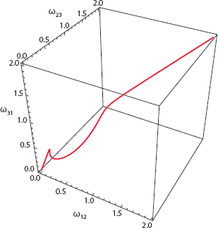
FIGURE 67. Affinity Trajectory
Case 3. Heterogeneous Exponents and Learning Rates
The out-of-equilibrium dynamics get more complex if we now add to the preceding different learning rates, the α’s, and β’s. If we simply call their product k, and set k1, k2, and k3, respectively, to 0.01, 0.04, and 0.08, the group’s affinity trajectory is very different, including a sharp hysteresis, as shown in Figure 68.
We will discuss link thresholds fully later. But, to anticipate slightly, let us assume—as seems defensible—that when the affective difference between two agents is sufficiently close to 1.0 (say 0.95) the link between them is broken. Under this interpretation, all these diagrams tell stories of endogenous changes in network structure (the pattern of links per se). Links dissolve, and then are re-established as affective differences rise and fall.
If we now move to the agent world and add a spatial distribution of stochastic aversive stimuli, the affinity and structural dynamics are more complex still and no equilibrium is assured. This is a central difference between the mathematical and agent models. A single example will suffice to illustrate the point.176

FIGURE 68. Affinity Hysteresis
Agent-Based Model: Nonequilibrium Dynamics
In fact, as we will see, in the spatial agent version, weight trajectories need not converge. Here is another example in which the mathematical and agent versions enrich one another. Without the mathematical version, one might not notice the convergent tendency in the first place. But with the mathematical version alone, you might never discover that divergence is possible. The agent model exhibits this. With both mathematics and agent-based modeling, you just learn more.
Case 4. Spatial Agents
To see the affinity dynamic in action, I present a familiar case. The run starts with all three agents in their initial positions before any attacks, with all connection weights initially equal to zero. Then attacks begin. These increase the v-values of the agents and, in turn, the interagent weights, which grow in the crucible of combat. The thickness of each link will equal the weight of that link. So, as these weights change through our affective homophily dynamics, so will the thickness of these links. Initially, the picture is as shown in Figure 69.177

FIGURE 69. Initial Weights Zero [Movie 9, start]
As things unfold, the experiences and affective trajectories of the agents begin to diverge. And the network structure encoded in the weights evolves accordingly, as shown (t = 500) in Figure 70.
Agents 2 and 3 develop the closest relationship, followed by that between Agents 2 and 1. Finally, when the entire yellow population has been annihilated, the agents’ pairwise relationships are not what they were before the war, as shown in Figure 71.
At this point, all aversive (Orange) stimulation has stopped and with it, any further change in weight. The entire evolution is recorded in Movie 9, on the Princeton University Press Website.
This equilibrium is sensitive to extinction rates. Here, affective extinction was zero. If the extinction rate is positive, then each agent’s affect eventually damps to zero; at this point their affective strengths are zero, as in turn are their weights, and the agents go their separate ways in life.

FIGURE 70. Endogenous Weight Dynamics [Movie 9, continued]

FIGURE 71. Endogenous Weight Dynamics [Movie 9, terminus]
As noted earlier, a general model should generate not only dark parables of baseless massacre but also parables of hope. And it does. An example unfolding at the time of this writing is the wave of anti-autocratic revolutions in the Middle East. A salient aspect of this so-called “Arab Spring” is the unprecedented central role of social media and endogenous networks in the dynamics.178 The Agent-Zero framework generates this parable also.
III.8. GROWING THE 2011 ARAB SPRING
Not all antiautocratic revolutions eventuate in functioning democracies. The Iranian revolution installed a theocracy, for example. The variant I am about to show, therefore, is meant to represent only the initial resistance and overthrow phases of a stylized revolution: the Tunisian, Egyptian, and Lybian revolutions of 2011 being recent examples. The long-term evolution of these political systems is not modeled.
Here we interpret the space as an initially monolithic ruling authority. The binary action available to the agents is to actively resist or not. Yellow squares are government entities—the police, the intelligence apparatus, government-controlled media, and so forth. Now we interpret orange activations as instances of government corruption (e.g., nepotism, bribery, abduction, human rights abuses). These are the stimuli that increase the agent’s affect V(t) against the government—by our usual Rescorla-Wagner mechanism. In addition, agents are sampling within their vision to estimate the relative frequency of orange—the probability P(t) of a randomly selected government entity being corrupt. Let us refer to the sum of these as the agent’s grievance. But, grievance alone does not a Molotov cocktail make. What is the risk of open resistance? The threshold term represents this.
If even the slightest expression of dissent will result in execution, the deterrent threshold τ is very high. On the other hand, if the direct open exposure of government corruption is tolerated, then the threshold is low. So, we can think of one’s total disposition as grievance minus threshold (similar to the Epstein Civil Violence Model179). But this is just our standard skeletal formula:
Of course, the entire point of suppressing freedoms of assembly and speech is to keep people in isolation. In the Arab Spring, social media played a huge role in thwarting these classic repressive measures, allowing networks to form and weights to increase to the point where dispositions to protest exceeded thresholds and the state was swept away in a flood of resistance (formerly dark red, now jasmine colored). Social media certainly did not create the underlying grievance. But, through dynamic network effects, it powerfully facilitated its amplification, emboldening the ultimately victorious rebels.
Let us generate this result in the Agent_Zero framework, beginning with no social media.
No Social Media
The left frame in Figure 72 shows our agents at t = 0. The right frame shows them in a sea of government corruption. With no social connection or reinforcement, the isolated Blue agents simply endure the ongoing corruption; there are no jasmine outbursts of resistance.
Although their antigovernment affect rises to its maximum possible levels (right frame of Figure 73), solo dispositions (since they are isolated) to openly resist do not exceed the risk threshold, and no rebellious action occurs. In sum, with all connection weights zero (left frame of Figure 73), no individual’s disposition can amplify any other’s. And despite antigovernment affect rising to maximal levels, no rebellious action occurs.
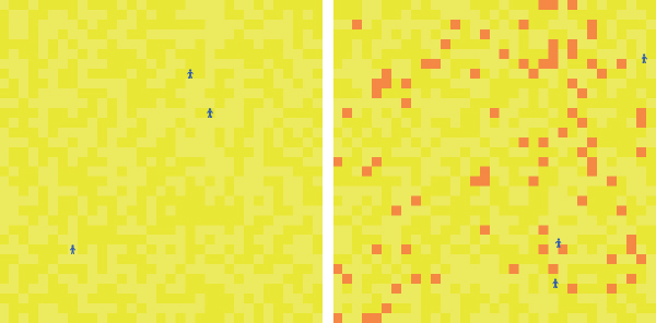
FIGURE 72. No Social Media

FIGURE 73. Weights and Affect with No Social Media
Endogenous Weight Adjustment through Social Media
If we now introduce the earlier apparatus of endogenous network weight adjustment, a radically different story unfolds. All other parameters are exactly as in the preceding run. But now weights can increase as before. The six panels of Figure 74 tell the story. In the upper two panels, we see connection weights growing through affective homophily (common opposition to the regime). Total (no longer isolated) dispositions thus come to exceed thresholds, and in the second pair of panels, local uprisings occur, replacing the government with jasmine.
Finally, in the third pair of panels, the jasmine revolution is complete and there are strong bonds among the victors. The jasmine revolution is recorded in Movie 10.
Notice, moreover, that with social connection, the level of antigovernment affect necessary to complete the revolution (Figure 75) is actually lower than the level attained in the earlier unconnected case where revolution never occurs (Figure 73).
Why is this happening in the model? It is because, during the course of the revolution, Orange stimuli (instances of corruption) are being overwritten (rooted out and eliminated) by jasmine patches (the damage radii), so the stimuli (the conditioning trials) are decreasing in frequency as the regime is eradicated. Hence affect never rises to the former level!180
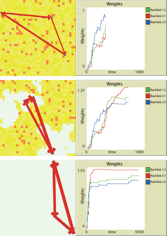
FIGURE 74. Growing the Arab Spring [Movie 10]
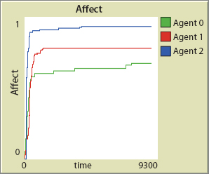
FIGURE 75. Affect During Revolution
Revolt of the Swarm
Perhaps the most remarkable thing about the Arab uprisings of 2011—and the feature that sets network effects into such sharp relief—is this: they have been leaderless. Name the Lenin, Mao, or Khomeini of the Tunisian or Egyptian Revolutions. Though ongoing at the time of this writing, the Libyan, Syrian, Yemeni, and Bahraini rebellions are equally leaderless. As if to echo Tolstoy, Engels famously remarked that “If Napoleon had been lacking, another would have been found.” But here, no alter-Napoleon is even necessary. It is truly the network—the swarm—that is making the revolutions. At the time of this writing, Occupy Wall Street demonstrations have spread widely around the world, also with no particular leader. Social media have made this possible, permitting affective (even dispositional) homophily to strengthen ties from the bottom up, and on a global scale. This is a fact fully appreciated by repressive regimes, of course, who—in many Arab countries—shut down Internet service to prevent organized rebellion. It is the Internet equivalent of a physical curfew. But freedom of cyber-assembly is a portentous development. It may usher in an age of leaderless revolutions.
In revolutions, existing legal systems are often destroyed. But the same Agent-Zero framework can be used to model legal systems in operation. In the examples thus far presented, emotional, deliberative, and social forces operate concurrently. In a trial by jury, certain of these are sequenced. Most distinctively, social interactions within the jury proper are forbidden until the jury is sequestered. At this point, powerful social effects are known to operate, driving jurors to conform to a majority (recalling the Asch experiment) as it unfolds behind closed doors. Of course, a complex emotional and deliberative evolution has already taken place for those who are empaneled. We wish to model three phases in the Agent_Zero framework: the pretrial public phase, the courtroom trial phase, and the jury deliberation phase. Each will be assumed to last 30 days.
Imagine a celebrity trial such as the O. J. Simpson case. Long before there was a courtroom trial, there was a vibrant public discussion of O. J.’s guilt. Let orange patches represent assertions of O. J.’s guilt. Yellow patches take the default position—innocent until proven guilty. Imagine three Blue agents who do not know one another and who have no idea that they are fated to become jurors. As they go about their business in the landscape of public opinion, they are bombarded with stimuli regarding the impending trial. In Figure 76 they are shown positioned randomly in the public space. The courtroom is the gray square that is empty in this phase of the process. One can imagine different neighborhoods with different modal attitudes toward O. J.
As usual, these stimuli are processed by our Blue agents. Their affect V toward O. J. is being driven by the flow of orange stimuli, just as before. And they are recording the ratio P of orange to observed patches as the crude empirical measure of O. J.’s culpability.
Employing the memory apparatus developed earlier, we assume that each Blue agent has a memory of 90, meaning that her most recent 90 probability estimates, or impressions, if you prefer, are stored.181 We also assume that the moving average over this sample is employed in forming her overall disposition regarding O. J.’s guilt. The P used in computing each agent’s disposition, in other words, is this moving average.

FIGURE 76. Landscape of Public Opinion [Movie 11]
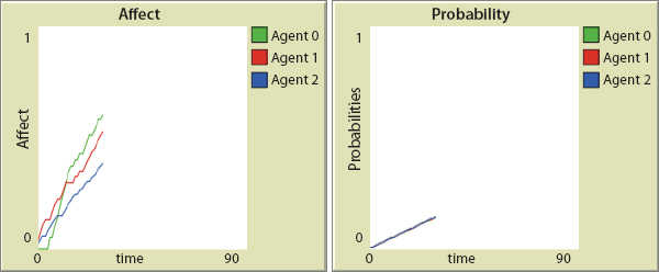
FIGURE 77. Affective and Deliberative Dynamics, Public Phase
These Phase 1 affective and deliberative components are plotted in Figure 77. Agents are exposed to effectively identical activation patterns, so their probability estimates are identical. But, because they have heterogeneous learning rates, their affects differ. These (minus their identical thresholds) are combined to produce in each agent a net disposition to pronounce O. J. guilty if asked. If this exceeds zero, they vote guilty; otherwise, innocent. Of course, this changes over time, as shown in Figure 78. At this point none of our jurors-to-be believe Mr. Simpson to be guilty.

FIGURE 78. Disposition to Convict Dynamics, Public Phase
Importantly, interagent weights are zero in this phase. The agents are still complete strangers. This is about to change.
Phase 2. Courtroom Trial Phase
We imagine that our three agents are chosen to become the jury in the court-room trial. Now the venue changes from the court of public opinion to the courtroom proper—the upper-right square. Previously, this was an empty gray, while the public area was alight with orange and yellow assertions. Now these landscape colors are reversed. As in Phase 1, interagent weights remain zero, since technically, jurors do not communicate in this trial phase. However, it is no longer the barber, the coworker, or the pundit who is offering orange and yellow stimuli. It is the lawyers for the prosecution and defense. Pursuant to rules regarding evidence, for example, the pattern of stimuli can change abruptly from Phase 1. Indeed, where Phase 1 may have generated a social majority opinion of guilt, evidence presented in court may favor the defense. Yellow (innocence presumptions) indeed outnumbers orange in the courtroom proceeding, as depicted in Figure 79.182
Whether this sways the jurors from their pretrial dispositions depends on a number of factors represented in the model.

FIGURE 79. Jury in the Courtroom [Movie 11, continued]
Extinction
Try as they may to suppress it, jurors often carry their pretrial affect into the courtroom. For some, emotions fade. In the language of the Rescorla-Wagner model, extinction occurs. In others it does not. Jury selection tries to weed out candidates who have an obvious emotional investment in one verdict over another. But, as we have already discussed at length, people may not be aware of their actual emotions, and despite appearing impartial under questioning, they may well harbor deep unconscious associations and presumptions of guilt or innocence. We can explore the effect of low and high extinction rates on the affective levels in place when the trial phase starts. Continuances may provide a time window in which some extinction can occur.
Memory
In the public pretrial phase, the agents will have formed probability judgments as well. Using the memory apparatus developed earlier, we imagine the jurors carrying forward a moving average of their estimates (relative frequency of orange within vision) over a memory window. For those with high memory, these pretrial probabilities will be insensitive to new data for a number of periods. Those with short memory will exhibit more rapid adaptation to the new courtroom evidence. For expository purposes, we will assume that all agents have memory 90 and that the moving average (rather than the moving median) over this window is the P-value used in computing each agent’s disposition to convict.
How much change occurs in these affective and probabilistic components also depends on the duration of the trial phase. As noted, I have divided the pretrial, trial, and jury phases equally at 30 periods. But, as in the real world, these can be quite arbitrary, and continuances and changes of venue may affect the course of events. The latter is explored later.
Finally, when all testimony and evidence for the prosecution and defense have been presented, the jury is instructed and sequestered in the jury chamber to arrive at a verdict. Now, for the first time, the jurors interact directly with one another. The social dynamics within juries can be very complex, with subnetworks vying for unattached jurors, who may join by affective homophily, or agreement on other dimensions. Here, we will focus on affective homophily, as modeled earlier. Just as before, inter-juror weights are given by the product of strength and homophily:
![]()
And, as before, each juror’s net disposition to convict is given by

If we depict the jury chamber as a small brown (oak-paneled) room, the picture of interagent weights and the sharp potential effect on verdicts is illustrated in Figure 80.
Some pairs are more closely bound (thicker links) than others, and the effect of weights can be huge, as shown by the sharp dispositional jump they induce, compared to the dispositions the jurors had before this phase. Weights are “off” until this phase but jump abruptly when affective homophily is discovered and bonds are formed, as depicted in the weight plots of Figure 81.

FIGURE 80. Jury Chamber [Movie 11, terminus]

FIGURE 81. Interjuror Weights
This can eventuate in sharp changes in the disposition to convict, compared to earlier phases, as illustrated in Figure 82.
Indeed, no jurors would have convicted before this jury phase, but they are unanimous in rendering a guilty verdict, having interacted directly. The entire history is recorded in Movie 11.

FIGURE 82. Jump in Conviction Dispositions through Endogenous Weights
The rationale for various well-known legal tactics emerges naturally from the framework. One of these is a change of venue.
Change of Venue
If a judge deems a fair and impartial jury to be impossible in a particular location, a change of venue may be granted and the proceedings moved to a community less affected by the crimes in question. The 1992 trial of Los Angeles police officers in the beating of Rodney King, for example, was moved from Los Angeles County, where the events took place (and were widely covered and inflamed the community), to Ventura County. As another example, having petrified the entire Washington, DC, area in 2002, the snipers John Muhammad and Lee Malvo were tried in southern Virginia.
The objective of changing venue is to minimize pretrial emotional bias. The present model suggests that the effect can be dramatic, but for a subtle reason. For example, in the preceding run, pretrial conditioning occurred and dispositions to convict were rising before the courtroom phase began (see Figure 77). A perfectly effective change of venue would eliminate this pretrial learning, and jury opinions regarding guilt would be based solely on courtroom proceedings. To capture this, we rerun exactly the same example as before, but without the pretrial stimuli. The result of this perfect change of venue is a concluding unanimous verdict of innocent, as shown in the terminal Figure 86 (four below). However, a number of mechanisms are involved.
Recall that, in the prior example, the courtroom evidence (in contrast to the court of public opinion) favored innocence. So, while some probability of guilt is assigned, it is low, as shown in Figure 83.

FIGURE 83. Probability of Guilt

FIGURE 84. Affect with Presentation of Evidence
Juror affects do rise with the presentation of evidence, but the levels are modest, as plotted in Figure 84.
Then the jurors retire to deliberate. Here they interact directly with one another for the first time. Their weights on one another depend on affective homophily, and those with similar feelings are mutually reinforcing. But, as indicated in Figure 85, the levels of affect, and hence the weights, are far lower than before (as also indicated by the lighter red links in the right frame).
This results in less dispositional amplification by homophily-based weight growth. In contrast to the previous unanimous guilty verdict, we now see a unanimous disposition to acquit! This is shown in Figure 86.

FIGURE 85. Weaker Dispositional Amplification and Lighter Network
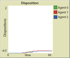
FIGURE 86. Unanimous Disposition to Acquit
Mechanism
Notice that, by our dynamic weight mechanism, the effect of a change of venue extends all the way into the private jury room. How? Pretrial affective growth is eliminated. So, only the affect accumulated in the trial phase proper is carried into the jury chamber. This is lower than it would be without the change of venue. But, because it is lower, the interagent weights—which depend on both strength and homophily—are also lower. These made all the difference before! Hence the intrajury momentum and peer effects, so decisive in the former run, are suppressed in this venue, resulting in a verdict of innocent. So, the model suggests that changes of venue may have unappreciated effects, shaping social dynamics within juries at times and places far from the scene of the (alleged) crime.183
III.10. EMERGENT DYNAMICS OF NETWORK STRUCTURE
One might define the term network structure as the continuous vector of interagent weights defined on [0, 2λ]. Typically, however, the term “network structure” is understood in the tradition of graph theory. Structure proper concerns the pattern of internode edges, or links, not their strengths. With some important exceptions,184 in this literature, links exist or not; it is a binary matter. And the analysis proceeds from there to study various statistics, such as the network’s degree distribution, clustering coefficient, and myriad other features.
We, too, want to study the dynamics of structure proper. How then can we map our continuous dynamics of connection strength—of interagent weights—onto a dynamic of binary structure? One solution explored here is to introduce thresholds and posit that a link exists if and only if the internode strength exceeds threshold. As we know from the foregoing, the time series of connection strengths based on affective homophily can be extremely spiky and volatile. But a link threshold filters these spiky dynamics onto binary {0,1} step functions, whose value is unity (i.e., a link exists) if the link threshold is exceeded and zero otherwise (no link exists). Mathematically, letting L(t) be the binary link function, and τL the link threshold, we simply define the Boolean link between Agents i and j as:
![]()
Equivalently, using the Heaviside unit step function introduced earlier, this is185
![]()

FIGURE 87. Episodes of Connection
This projects the continuous strength dynamics on the real interval [0, 2λ] onto a discrete structure dynamic on the binary set {0, 1}.186 Structure thus emerges as a kind of projection, or filtered version, of underlying connection strength dynamics. So, the model crudely addresses the questions: Why does network structure happen? And why might it change?
As an example, in the time series of Figure 87, we define weights as in equation [52]. Weights vary between 0 and 2. If the link threshold (black) is set to some intermediate value, we see that links form and dissolve as the undulating affinity landscape rises above and falls below the threshold. There are some fully connected periods (where all weights exceed threshold), some completely disconnected episodes (where none do), and some episodes in which only two of the three nodes are connected, as where only the green curve (the link between Agent 0 and Agent 1) exceeds threshold.
Networks “happen,” in other words, when weights “break the surface” defined by these thresholds, as suggested in Figure 88, with a blue subsurface.
Network Structure Dynamics as a Poincaré Map
Thus we see that network structure as classically defined (binary) is an epiphenomenon of underlying similarity dynamics (continuous). It is a suspension,187 somewhat analogous to a Poincaré map. The threshold is the Poincaré section. These breachings of the surface (the threshold) generate the discrete time return map of an underlying continuous dynamic. [On Poincaré maps, see Guckenheimer and Holmes (1983), Wiggins (1990), Strogatz (2001), and J. M. Epstein (1997)]. In this view, then, dynamic network structure is the binary (step-functional) projection of an underlying continuum affinity phenomenon.
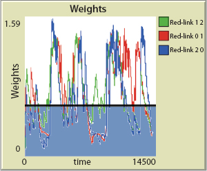
FIGURE 88. Networks with Threshold

FIGURE 89. Network Dynamics on Affective Similarity
Obviously, the binary dynamics of network structure change if we change the link threshold (the Poincaré section). Figure 89 shows the surface just depicted as the middle threshold, but with a higher and lower one shown as well. Given the lowest threshold, the network is fully connected throughout. As all this is happening, the degree distribution of the network and innumerable other measures of connectivity are also changing.

FIGURE 90. Network Dynamics on Cognitive (Probability) Similarity
This is network dynamics on affective (V) similarity. But using the same algebraic form of equation [52] with P instead of V, one could study network dynamics on cognitive similarity—that is, on the similarity of probability estimates on the same landscape. That picture is given in Figure 90, also with three thresholds.
However, unlike the high-threshold dynamic on affect, the high threshold (upper black line) here produces disconnection at essentially all times. Comparing the low threshold cases, on affect full connection obtains; while on probability, there are many (and well-packed) periods of complete disconnection. This comparison suggests what is, of course, true: some of our affect-based networks (dog lovers) may be thriving while deliberation-based networks (chess clubs) are in decline.
Many other network visualizations are possible. Obviously, one can literally draw links forming and dissolving as agents interact spatially. Thinking again of affective homophily, if we posit a link threshold of 0, full connection obtains; while at a threshold of 1, connection is extremely sparse. Movie 12 shows an animation of connection dynamics at an intermediate threshold of 0.5. Here connections form and break in the course of the run. (All code, once again, is provided on the Princeton University Press Website). The upper-left frame of Figure 91 shows the agents on a completely quiescent landscape. Since there is no stimulation, affect remains 0, so connection weights are also 0. Connectivity changes as agents move into and out of stimulus zones, as shown in the other three frames, captured at arbitrary times. Of course, weights never decline if there is no affective extinction rate. Here, we assume a positive extinction rate.188 In yellow zones, there is no stimulus, so affective extinction is unchecked. This can lead to link weakening and breakage, as in the right frames.

FIGURE 91. Endogenous Network Structure. [Movie 12]
Another visualization of structural dynamics is to display the derived step functions themselves. We illustrate this in stages.
First, for arbitrary parameters, we give time series of raw affect itself (Figure 92).
Second, in Figure 93, we plot the weights on affective similarity (as in equation [52]) with no binary filter—that is, no L-function introducing a link threshold and mapping values to {0, 1}.


FIGURE 93. Dynamic Weights
The next three figures, Figures 94–96, give this weight plot, filtered to produce different dynamic network-structure trajectories. The first sets the link threshold to 0.25, meaning a link is established if and only if the weight (ωij) exceeds 0.25. Since this is relatively weak, the network quickly becomes fully connected and stays that way. Note that a link exists if the value is 1 and does not exist if it is 0. I include the range −1 to 2 rather than only the operative range, 0 to 1, merely for visual clarity. All the action is on {0, 1}.
Link Threshold 0.25
Periods of full connection become rarer as we hike the link threshold to 0.5.

FIGURE 94. Threshold 0.25
Link Threshold 0.5

Finally, disconnection dominates at threshold 1.0, with no periods of full connection, as shown in Figure 96.
Link Threshold 1.0

FIGURE 96. Threshold 1.0
Network Structure an Epiphenomenon of Affinity Dynamics
So, in this conceptualization, underlying affective dynamics (grounded in a classic learning model on a dynamic landscape of stimuli) generate time series of interagent weights (based on a strength-scaled homophily measure). But this same weight dynamic generates network structure proper (the pattern of binary edges and nodes) when it is mapped onto a binary step function through a link threshold. Each different link threshold generates a different dynamic network structure for the same affective affinity evolution, just as a different Poincaré section may generate a different return map for a fixed dynamical system.189 Agent behavior (to rebel or not) depends on total disposition minus the action threshold. As we have shown, each dispositional trajectory (and hence action history) is compatible with many different dynamics of network structure, defined narrowly as the set of binary internode connections. Every choice of a link threshold selects one of these dynamic evolutions of network structure proper. In the Arab Spring example, if one posits a threshold of zero, then full connection occurred very early in the affective dynamics.
The preceding model of attachment by strength-scaled homophily (whether affective or probabilistic) offers a completely different network formation mechanism than preferential attachment (PA). There, the probability of a new node attaching (making an edge) to a node k is proportional to the latter’s degree—the number of nodes to which k is already connected. Thus, well-connected nodes enjoy an (increasing) advantage in collecting new partners. The idea has a long mathematical lineage.190 In 1976, de Solla Price introduced a general cumulative advantage distribution to explain dynamics in which “success seems to breed success.”191 In 1999, Barabasi and Albert (1999) presented a model in which PA was shown to generate scale-free power-law degree distributions observed in many large networks, including the World Wide Web.
It may well be that PA has been a central mechanism in the formation of the World Wide Web. But, in many contexts, and in my preceding model, attachment is unrelated to degree, depending instead on an associative dynamic.
Degree-Independent Attachment Models and an Hypothesis
In research on the coevolution of networks and political attitudes, Lazar (2001) uses the absolute value of an attitudinal (though not literally affective) difference as his measure of political similarity, and establishes empirically that “homophily in political views contributes to tie formation.”192 In a different study, Levitan and Wisser (2009) demonstrate a strong correlation between attitude strength and social ties. This relationship, like Lazar’s, is unrelated to degree. But unlike Lazar, they ignore homophily. My model includes both a strength term (e.g., the sum of affects) and a homophily term. I certainly would not claim that either of these studies directly tests my model (or even defines terms in exactly the same way). But the model does offer a testable hypothesis, namely, that ceteris paribus, the tie probability increases with the product of affective strength (vi + vj) and affective homophily, 1 − | vi − vj |.
It would, of course, be interesting to see whether a scaled-up version of the model could generate the observed dynamics of real-world networks or simply generate known network structures, such as are hypothesized for obesity, smoking, and other behaviors.193
My exposition here has been predominantly on affective strength and homophily. But it could be on similarity of probability measures, or dispositions, or spatial proximity, as well. Again, for various link thresholds, these would generate a diversity of network structure dynamics that could be compared to data.
Albeit crudely, this captures a central fact about people. We belong to many networks at any one time. We can belong to a network based on data and empiricism, P(t), and an entirely different network based purely on emotional, V(t), similarity. They are both dynamic and may overlap at various times, or not. To expand on Spinoza, then: we are not just social animals. We are many social animals at once!
While many of the earlier computational parables have been dark, the parable of the Arab Spring shows that, unlike economics (discussed further shortly), the science of Agent_Zero is not necessarily dismal. Lynchings and liberations are both generable.
III.11. MULTIPLE SOCIAL LEVELS
Now, all examples thus far involve the activation of the yellow spatial sites. Call these the Level_1 activations. Then Level_2 agents take these as their Rescorla-Wagner conditioning trials and take actions accordingly. Thus far, only those two layers have been in play. But there is no reason to stop there. One could posit Level_3 agents who take the deeds of Level_2 agents as their stimuli. They train on those stimuli by the same general Rescorla-Wagner scheme and also act accordingly. Presumably, their behavioral repertoire—their possible actions—would be qualitatively different from those of Level_2 agents (e.g., they might have the option of regulating Level_2 agents). This process of adding levels can, of course, be continued. In general, the deeds of Level_n agents are the stimuli for Level_(n + 1) agents. A concrete example for two levels follows.
Agent_Zero as Witness to History
Recall our very first parable, the slaughter of innocents. For the perpetrators of slaughter, the stimuli (the Rescorla-Wagner training trials) were the orange activations on the landscape, interpreted as attacks by insurgents. When the perpetrator’s threshold was exceeded, he indiscriminately wiped out all patches—orange or yellow, guilty or innocent—within some destructive radius, coloring them a dark blood red. That was the end of it. No agents ever came along and took the dark red patches as their stimulus. Let us introduce such an agent—she could be a UN peacekeeper. We color her green, as shown in Figure 97.

FIGURE 97. Level 2 Green Agent
For this agent, it is not the orange patches, but rather the blood red ones (the dead, in other words) that are her training trials. Activations on the landscape (Level_1) stimulate the Blue perpetrators (Level_2); their deeds stimulate our Level_3 Green agent. She roves the landscape like the two Blue perpetrator agents. She may come upon killing fields in the course of her random walk. She updates her affect exactly like all other agents—according to the Rescorla-Wagner scheme—but the other agents’ victims (the dark reds) are her stimuli, not the orange patches that stimulate the killers. Every time she sees a red patch (a dead agent), she updates her affect. We record this event by having her paint the patch grey. (You may imagine that she erects a grey tombstone or, more likely, files a grey report).
Illustrative Run
In this run, it takes her (a Level_3 agent) a while to discover the terrible truth about what is happening at Level_1. In this particular random walk, she hasn’t encountered any killing fields at the point shown in Figure 98.

FIGURE 98. Killing Fields Not Yet Discovered (links for visualization only)

FIGURE 99. Killing Fields Marked
But eventually she does. Soon, she encounters killing fields, begins updating her affect, and begins marking the killing sites (Figure 99), perhaps to document events for the Level_4 International Court of Justice in The Hague.
Even at this stage, her (Green) Rescorla-Wagner acquisition curve is flattening out (Figure 100). Her associative capacity is approaching its limit, and each new discovery is less impactful than the last (diminishing marginal impact is evident, in other words), even as she paints the world grey (Figure 101).194
This, of course, is but one multilevel interpretation. The dark red patches could be vaccines refused and the Green agent a public health authority observing instances of this behavior—and becoming energized (through Rescorla-Wagner updating) to intervene and change it. Or the dark red patches could be assets abandoned in a financial panic, and the green agent the Federal Reserve growing ever more fearful of deep economic repercussions.

FIGURE 100. Affective Dynamics

FIGURE 101. Holocaust Revealed
The point is that, in the main exposition, we have not gone beyond the dark red patches (jasmine for the Arab Spring). But they can themselves serve as the stimuli for a higher layer of agents, whose actions (grey patches) can serve as stimuli for a yet higher layer, and so on. We can add layers recursively in this way to build up a multilayered model in addition to the two-layered (patches and rover agents) one that has been our focus. Within each layer, moreover, social dynamics can unfold through weights and homophily, by the same apparatus we’ve used at the lowest agent level. As emphasized earlier, the Rescorla-Wagner model applies not only to fear but to other emotional learning. So, one layer could be growing more fearful through its learning dynamic, while a different layer could be growing more happy.195 All in all, a society of tremendous depth and richness can be generated in this recursive fashion, with different network, action, and emotional extinction dynamics unfolding at the different levels. One could even allow Level_n agents to reach down and act directly on agents far below them in the hierarchy. All this strikes me as an important line of future work.
III.12. THE 18TH BRUMAIRE OF AGENT_ZERO
To this point, agents have not had offspring. Many agent-based models include some form of reproduction. Some have also explored the intergenerational transmission of genes, cultures, and immune systems, idealized in various ways (Epstein and Axtell, 1996; Miller and Page, 2007, Ch. 10). Here, let us attempt something different, an intergenerational parable inspired by Marx. In The Eighteenth Brumaire of Louis Bonaparte (1869; 1972 ed.), he writes,
Men make their own history, but they do not make it just as they please; they do not make it under circumstances chosen by themselves, but under circumstances directly encountered, given, and transmitted from the past.
Then, inimitably, he writes,
The tradition of all the dead generations weighs like a nightmare on the brain of the living.
How might we interpret and generate this parable in Agent_Zero? The first (nonitalicized) passage requires that agents be born into preexisting circumstances. This we can represent by having them begin life in the immediate (von Neumann) neighborhood of their parent, ensuring that their “directly encountered” environment is, as per Marx, not of their own choosing. His (italicized) continuation, however, is the enticing and more elusive part, the idea that parents transmit a “tradition” that “weighs” on their offspring.
Transmission of Chronicles
How might we get at this? As a crude beginning, recall that, in each period agents are making a social appraisal, “calculating,” as it were, the relative frequency of enemies (orange) within their vision. Employing the memory apparatus developed earlier, they carry a string of the m most recent such appraisals. We have called m the memory length and the string that agent’s memory. Parents do, in some sense, impart memories to their children—chronicles of their culture’s achievements, its persecutions, its days that will live in infamy. The parent may be gone, but the parent’s story, her chronicle, her “tradition,” if you will, lives on in the offspring. While we inherit our parents’ chronicles, we also leave home, have new experiences, and accumulate a new string of social appraisals. The parental nightmare—distrust of yellow sites, for instance—can be overwritten by happier stories, or—to be sure—by new nightmares! We will tell the happier parable in code.
To wit, we imagine the world as divided into a hostile north and a peaceful south. The parent lives her life in the violent north (as in the upper left panel of Figure 102). Accordingly, her narrative (her period-10 memory string) consists entirely of high values—appraisals of high likelihood that any agent within vision is an attacker, an enemy.
At a randomly chosen time, she clones an offspring. The parent passes an exact copy of her memory—her experiential chronicle—to the child. And then she expires (her grave is marked by an X in the right panel), becoming Marx’s dead generation. So, at this moment, the “tradition of the dead generation weighs like a nightmare on the brain” of our newborn. But the child begins to move away and begins to overwrite the inherited chronicle with his own. Eventually, after some time in the violent north, the child migrates to the sunny south (Figure 103), where his experiences are all peaceful (run the Applet on the book’s Princeton University Press Website to generate this spatial history).
His social appraisals eventually overwrite the transmitted story of yellow hostility until he is liberated from it. The dead generation’s nightmare is lifted.
The story of this awakening is recounted in his memory strings, which begin with a duplicate of the parent’s nightmare. But through migration and new experiences, zeros invade. The parental nightmare is ultimately displaced by a narrative of peace (all red zeros), as shown in Figure 104.


FIGURE 103. Migration
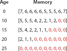
FIGURE 104. Inherited Chronicle Overwritten
The particular story is not as dismal as Marx’s. But we will turn now to what Carlyle dubbed “the dismal science,” economics.
III.13. INTRODUCTION OF PRICES AND SEASONAL ECONOMIC CYCLES
In very general terms, we have discussed a number of economic interpretations of the model: contagious financial panic, fear-inspired dumping of assets, and capital flight. But, we have not introduced prices in any explicit way. And, to economists, prices are the sine qua non of true economic models. But, prices are so easily introduced that a brief discussion is warranted.196
The general model, recall, would apply to settings where decisions depend on affect (passion), calculation (reason), and social network effects. In choosing products (e.g., a brand of ice cream), the associative strength of its consumption with pleasure v, our calculation of its health implications (probability P of diabetes given consumption), and the prevalence of consumption among my weighted friends all enter in. But, obviously, so do prices. The natural place to introduce them is in the threshold term. Let us imagine the binary action of interest to be the purchase of some good197 and make the threshold a nice orthodox convex function of exogenous price (p). Specifically, set

All else fixed, consumption decreases as price increases, because the threshold rises with price, but it does so at a diminishing marginal rate.
The economist, Wesley Mitchell (1927, p. 236) wrote that, “Two types of seasons produce annual recurring variations in economic activity—those which are due to climates and those which are due to conventions.”
As a trivial conceptual demonstration of the former, consider the demand in New Zealand for fresh fruits and vegetables—apples and kiwi fruit, for example. Local production stops for winter. So, the price increases to cover transportation costs from elsewhere. Seasonal fluctuations in price result, as shown in Figures 105 and 106.198
Ceteris paribus,199 demand and price move in opposite directions, so these price fluctuations generate anticorrelated demand dynamics. Thinking of disposition as the disposition to purchase at prevailing prices (so, as in neoclassical perfect competition, Agent_Zero is a price taker), we can easily mimic this cyclical demand dynamic by forcing the threshold seasonally. As an off-the-shelf function, I have let the threshold vary as the cosine of elapsed time, as is often done in modeling seasonal epidemics (J. M. Epstein et al., 2007; Earn, Rohani, Bolker, and Grenfell, 2000; Koelle, Pascual, and Yunus, 2005; Ellner et al., 1998; Aron and Schwartz, 1984). This produces the inverse “price-demand” cycles shown in Figure 107.200
Prices and demand are negatively correlated and cycle periodically, as in the fresh-fruit examples.
Exogenous Climatic Variation
In this example, seasonally varying production costs are driving the price fluctuations. It is more expensive to produce, refrigerate, and transport this commodity, fruit, from Florida to New England in winter than to produce and consume it locally in New England in the summer. And these increased winter costs are passed on to consumers as a higher price in New England. In the argot of textbook economics, the supply curve shifts left raising (equilibrium) prices at each quantity of output.201
Apples
September 2004—November 2009

FIGURE 105. Apple Prices. Source: Statistics New Zealand Tatauranga Aotearoa
Food Price Index
Kiwifruit
September 2004—November 2009

FIGURE 106. Kiwifruit Prices. Source: Statistics New Zealand Tatauranga Aotearoa
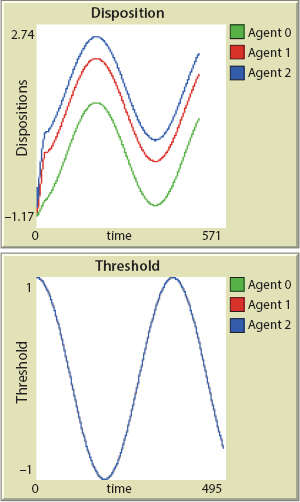

FIGURE 108. Demand for Sporting Goods Spikes at Christmas: eBay Category Trends (skiing and snowboarding).
Endogenous Conventional Variation
However, changes in demand (rather than supply) can occur due to seasonal fluctuations in affective dynamics, holidays being a prime example; these are Mitchell’s “conventions.” Skates and snowboards presumably cost no more to produce in December than in June. But their prices spike at Christmas. In this case, affect and the disposition to purchase are seasonally forced. There is also clear extinction of affect after the stimulus of the holiday is turned off, and the price data show a decrease accordingly. See Figure 108, depicting the annual spikes in Christmas sales of sporting goods.
Seasonal Demand
How shall we generate this in the Agent_Zero model?202 We will exercise the model in yet another way, allowing the landscape to oscillate seasonally. But we now interpret our space as the shopping district of a major city. Yellow patches are products of any sort. Orange patches are products that are Christmas specific and/or bear Christmas-specific advertising. In the former (Christmas-specific) category would fall Christmas trees (real or artificial), decorations, lights, electric plastic Santas and reindeer for your roof, and Christmas carol CDs. Products that are not Christmas specific but bear Christmas-specific advertising could include skates, bikes, sleds, and holiday hams,203 seasonally festooned with red and green ribbons.
These orange activations are the stimuli associated with the season, and they increase v.204 The same process also increases P, the local relative frequency of orange. We interpret this as the probability that, when you walk into a mall, for example, you will encounter a Christmas purchase candidate—either Christmas specific or strongly Christmas associated through advertising. As usual, v and P combine to produce a purchase disposition that is compared to a threshold (that can be price dependent, as above). The dispositions of other people also have weight and are detectable by their holiday clothing, caroling, gift-laden shopping bags, and text messages and cell-phone calls about good deals just around the corner (which we would thus include in the agent’s “vision,” or shopping radius). These are the weights, ωji. As per the familiar skeletal equations, all this is added up and compared to the individual’s action (purchase) threshold. If total disposition exceeds τ (or τ(p) as before), the shopper takes binary action, buying all items in some radius. If the radius is 0, she buys only the orange product. If the radius is 1, she might buy a Christmas-specific sweater (orange patch) but also a generic Burberry’s scarf and hat (yellow patches). The shelves where these items were stocked are colored dark red, indicating “sold.” Stimuli and dispositions drop sharply after the holiday, the Christmas tree lights go back in the attic, and in the off-season the shelves are restocked and the cycle repeats again the next year. We generate this “Christmas tale” next.
Before Christmas season we see our three erstwhile shoppers walking randomly around the Upper East Side against a background of yellow off-season shopping opportunities (left panel, Figure 109). But as the Christmas season begins, the landscape lights up with seasonal offerings, shown in orange (middle panel, Figure 109).
And before too long, affect and probability drive dispositions over the shoppers’ (heterogeneous) thresholds and the shopping sprees begin, leaving a trail of empty shelves (dark red) where our agents have made purchases, as shown in the rightmost frame. Christmas offerings and other seasonal stimuli then end, the landscape reverts to yellow (as on the left), the probability of finding a Santa suit for sale drops precipitously, and the holiday affect slowly wanes (extinction)—and with it, the Christmas-specific buying disposition. The cycle repeats on an annual basis, as shown in the three panels in Figure 110, giving probability, affect, and net purchase disposition for our three (heterogeneous) agents over three roughly 365-day years.

FIGURE 109. A Christmas Cycle [Movie 13]
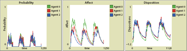
FIGURE 110. Deliberation, Emotion, and Disposition to Purchase over Three Christmas Seasons
In Movie 13, posted on the book’s Princeton University Press Website, you will see different spatial patterns of available products and buying each season.
Aggregate demand (the sum of all net dispositions) over two years is shown, in Figure 111, to very crudely mimic the previous two-year sporting goods sales data.
Given sufficient action radii, it may be that very little Christmas-specific advertising is required to “tip” the system into seasonal consumption spikes. The framework allows exploration of this possibility.205

FIGURE 111. Cyclical Aggregate Demand
Serial Dispositional Satisficing
One could extend this by endowing each shopper with an initial budget, B0, which simply depletes as purchases are made. At any time, the agent’s net budget is simply the amount remaining. Net disposition to purchase an item at a given price, p, is D − τ(p), as before. Purchase opportunities are encountered at random as the agent moves about the shopping-scape, and purchases are made serially whenever the following simple satisficing206 condition is met: net disposition and net postpurchase budget are both positive.207 One could even complete this bare-bones sketch by modeling patches as firms owned and operated by Agent_Zero–type CEOs, who set prices (p) to cover costs and reap profits.208
Neuromarketing
Beyond holiday cycles, one can see how a neuroeconomically sophisticated producer would seek to maximize Agent_Zero’s disposition to consume her product. The model quite naturally reflects that producers can focus their advertising on affect (“Campbell’s soup is mmmmm good”) on health deliberation (Healthy Choice soup is low fat), on social appeal (“Nobody doesn’t like Sara Lee”), on prices (“Buy one, get one free”), or some mix of these.209
In any case, my earlier remarks about using the Agent_Zero framework to study financial contagions, the collapse of spatially explicit housing markets, or other cascading economic dynamics is far from idle. Given relevant data, the replication of historical episodes—economic and otherwise—could profitably be attempted. This may inspire the collection of relevant data, both economic and neurocognitive.
III.14. SPIRALS OF MUTUAL ESCALATION
As a concluding extension, I would like to “close the circle,” harking back to our opening examples of violent occupation by Blue Agent_Zero actors. Thus far, the patches—interpreted as a yellow indigenous population—have not been endowed with any agency. They simply go active (turning orange) at an exogenous user-specified rate. And, thinking of the opening civil violence examples, they don’t retaliate on their occupiers in any way. They can’t “shoot back,” as it were. Here, I will add both these elements of agency—adding an endogenous attack (i.e., rebellion) rate and the ability to return fire—in the simplest way. This will permit us to generate mutual escalation spirals.
Of course, both colonial and military history are full of cases in which repressive force by occupying powers has exacerbated underlying grievances. The occupier destroys the landscape and infrastructure and kills innocent civilians. This backfires and produces more rebels. These new insurgents inflame the hostile passions of the occupiers, who respond with more indiscriminate violence, producing more civilian casualties, which begets further rebels, in an upward spiral of mutual escalation. One has only to think of the current (2012) events in Syria as an immediate example, though history is replete with others. Sometimes the rebels prevail, and sometimes they are wiped out. These spiral dynamics and various outcomes can be quite naturally generated from the core model with a few simple alterations.
Endogenous Attack Rate and Retaliation
As before, the Blue occupier’s affect grows (à la Rescorla-Wagner) with aversive stimuli (rebel attacks). We apply the earlier-developed extension wherein the occupier’s damage radius increases with his affect.210 As this damage radius increases, so does the level of general destruction (including innocent civilians). Now we introduce our two extensions.
First, the attack rate itself (the frequency with which quiescent yellow patches go active, turning orange), which had been constant,211 now grows with the level of destruction.212 But this endogenous rebel attack rate produces a feedback effect: the higher indigenous attack rate produces a higher occupier affect, in turn producing a greater damage radius and more indiscriminate destruction. This produces a higher insurgent attack rate, inspiring more indiscriminant destruction, more insurgents, and so on, in the upward spiral. But who wins?
Thus far, the yellow patches have not been permitted to return fire. So, the second extension is to now assume that when a patch goes rebellious (turns orange), it has some user-specified probability213 of killing any occupier within range.214 We arm the patches and let them return fire. Mao’s famous dictum was that revolutionaries must “swim like fish in the sea,” vanishing into the general population (returning to the yellow appearance) after each openly rebellious act. Our rebels will do likewise.
These alterations suffice to generate upward spirals and the core result in which, unlike the opening parable of unbridled rampage, the rebels succeed in defeating the occupiers. As an existence proof (not a full robustness analysis), I offer the run of Figure 112.
Panel 1 (upper left) shows sporadic opposition activity before any destruction by occupiers. As destruction progresses, the rebellious attack rate itself grows, as shown in panel 2 (upper right). However, the Blue destructive radius also grows as the frequency of insurgent attacks increases. When their destructive radius reaches 2, the occupiers can destroy sites without actually stepping on them—from inside a protective radius—as also shown in panel 2. Notice that, operating from within these enclaves, the Blue agents are not subject to any direct stimulation. So, their affect does not update in the Rescorla-Wagner model. They continue killing with literally flat affect. However, the insurgents are assumed to have weapons that can reach 1 unit into these enclaves. So, when a Blue gets near an edge, he is vulnerable to the insurgent orange sniper (who, as per Mao, turns yellow again with some probability). One of the Blue occupiers has been picked off in panel 2, and a second in panel 3 (lower left). Finally, with half the country destroyed, the occupiers are thwarted (panel 4). At this point, most of the country is radicalized (orange). The remaining yellows are a mix of recent members of la resistance and remnants of the ancienne regime pretending to be. The entire revolution is shown in Movie 14.

FIGURE 112. Successful Revolution [Movie 14]
The insurgent attack rate has grown throughout, as evidenced by the increased frequency of orange sites. The plot of attack rate over time is clearly increasing, as shown in Figure 113. It rises from 10 to 52, a 5.2-fold in-crease. But this and the damage radius are closely coupled. In fact, tracking the Blue agent who lasts longest, his damage radius begins at 0.3 and ends at 1.6, a 5.3-fold increase. Escalatory mutualism is clear.
In a full extension the yellow patches would be Agent_Zero agents in all their glory, endowed with the same affective, deliberative, and social apparatus as the Blue occupiers. They would have a disposition to retaliate that could be affected by homophily dynamics (shared antioccupier affect for example) and endogenous network structure, as explored earlier. This full generalization is suitable for future research. Here, however, is a simple step in that direction which—by endowing the patches with minimal agency—generates the upward mutual escalation dynamic observed in many rebellions and anticolonial struggles. In addition to endowing all patches with agency (making them all Agent_Zeros), numerous lines of future research strike me as fertile.

FIGURE 113. Endogenous Rebel Attack Rate
152The coding change required to endogenize the destructive radius as a function of positive affect is trivial:
to take-action
ask turtles [
if disposition > 0 [ask patches in-radius (affect * 10) [set pcolor red − 3]]
]
end
Here, 10 is just a scaling factor and destruction is color-coded as pcolor red-3.
153For a well-researched popular account, see Mnookin (2011).
154Regression of dopamine receptor density on BMI exhibits a negative linear relation (Wang et al., 2001).
155To generate this particular picture, use the Applet provided on the Princeton University Press Website, with a random seed of 2, as per Appendix IV.
156Haegerstrom-Portnoy, Schneck, and Brabyn (1999).
157Harms, Cooper, and Tanaka (2011).
158The subscript order is reversed to suggest that, unlike the experience of weight, Agent 1 is actively imputing a value.
159Of course, each run of the model is a single sample path of a stochastic process. And we should never assume a particular realization to be statistically representative. But, in this case, we will prove analytically that the central ordering holds up for positive threshold imputations.
160Assuming monotonicity in time, of course—a weak requirement.
161This follows from equation [40]. With V2 = P2 = 0, the requirement becomes ![]() which exceeds τ1.
which exceeds τ1.
162See Smith and DeCoster (2000, p. 108): “Humans possess 2 memory systems. One system slowly learns general regularities, whereas the other can quickly form representations of unique or novel events.”
163The agents are motionless and their spatial sampling radius is 4.
164This is used, for example, in the game theoretic model of Best Reply to Recent Sample evidence (Axtell, Epstein, and Young, 1999, pp. 191–211).
165Technically, a moving average (MA) can also show decay. Suppose that we remember the most recent six events and that we receive a string of exactly six values, each of which is a 1. Assume that, from then on, we get no new input. How does the moving average evolve? The opening memory array would be (1, 1, 1, 1, 1, 1), and its MA is ![]() = 1. Then the array is (0, 1, 1, 1, 1, 1) and the MA is
= 1. Then the array is (0, 1, 1, 1, 1, 1) and the MA is ![]() . Next period, memory holds (0, 0, 1, 1, 1, 1), and MA =
. Next period, memory holds (0, 0, 1, 1, 1, 1), and MA = ![]() . Then the values will be
. Then the values will be ![]() , and, finally, 0. So, it does decay. For a point event, it simply drops to zero, and some form of weighting, such as exponential, could be introduced. It would then be interesting to explore cases where this exponential decay and the exponential decay of affect differ in various ways or are equal, a suggestion for which I thank Robert Axelrod. Obviously, I am not claiming to have resolved this issue, only to show that the Agent_Zero framework includes memory, and can accommodate a wide range of treatments.
, and, finally, 0. So, it does decay. For a point event, it simply drops to zero, and some form of weighting, such as exponential, could be introduced. It would then be interesting to explore cases where this exponential decay and the exponential decay of affect differ in various ways or are equal, a suggestion for which I thank Robert Axelrod. Obviously, I am not claiming to have resolved this issue, only to show that the Agent_Zero framework includes memory, and can accommodate a wide range of treatments.
166Here, we return to the form without any imputation of thresholds. As the latter are constants, they do not affect the derivatives of interest here. Neither do the thresholds; this derivative will be identical to that computed on net disposition.
167If Pj = 0, the entropy is 0 by convention, since technically the ln P term goes to negative infinity as P approaches 0.
168Ceteris paribus, the same random seed (here equal to 1) will produce identical runs.
169This is a statistically complex matter when dealing with data (Shalizi and Thomas, 2011). Of course, we know the mechanism is homophily here.
170Notice that there are only three links because the functional form imposes the symmetry hij = hji. The same will hold for weights, ωij.
171One could normalize by 2 to bound weights to the unit interval, but at this scale it’s cleaner not to.
172As earlier noted, it is clear that ωij = ωji.
173The limiting value as t approaches infinity.
174Normalization to eliminate the 2 introduces unnecessary clutter at this 3-agent scale.
175x(∞)denotes the limit, as t approaches infinity, of x(t).
176Other weight-adjustment schemes are suitable for a longer study.
177Numerical values used are given in the Appendix IV table of assumptions and are also available from the Source Code in the Applet.
178This is not to deny an important role for the “social media” of the day in earlier bottom-up revolutions. Samizdat in the USSR, Cato’s Letters in the American Revolution, and audio cassettes of Khomeini speeches in Iran would be examples.
179J. M. Epstein (2002).
180This mechanism is reminiscent of the fight-vs.-flight example, in that stationary fight eliminates stimulus, whereas flight requires passage through a stimulus-rich environment. When actions endogenously change the environment, counterintuitive results may occur.
181In this 90-day process, therefore, all probability estimates are remembered.
182Hence, the relative frequency of orange is lower than in Phase 1.
183It is interesting to compare jury trials to elections. The perfect change of venue eliminates Phase 1—the public square phase—of the dynamic. The voting booth removes Phase 3—a nonanonymous voting process. In an election, the analogue of the public phase is the precampaign jockeying and buzz around potential candidates. Then there is the formal phase of official campaigning and formal debate (a term I use advisedly), the “courtroom,” where candidates present their respective cases. But then, votes are cast privately in the voting booth. So, the momentum of the jury room itself (Phase 3) is minimized.
184Famously, Granovetter (1983) distinguishes between weak and strong ties. These do not change dynamically.
185By the symmetry of formula [52], Lij = Lji.
186If one wanted an everywhere differentiable version, one could define L as a sigmoid of ωij confined to the range [0,1] and tune the function to differentiably approximate the step function as closely as desired.
187See Jackson (1992).
188See the Appendix IV table of numerical values.
189The converse does not obtain. Different dynamical systems could generate the same return map, given a fixed Poincaré section. The same holds for binary network structure in this model. If one doubles all amplitudes with frequency fixed, the continuous dynamic is different, but its binary projection is not.
190See Simon (1955) and Yule (1925).
191See Price (1976).
192See Lazer (2001) and Carpenter, Lazer, and Esterling (2003).
193See Christakis and Fowler (2007) and the methodological literature surrounding their work, beginning perhaps with Lyons (2011) and Shalizi and Thomas (2011).
194This brings to mind the important phenomenon of “psychic numbing” documented in Slovic (2007).
195I thank Julia Chelen for this thought.
196Again, detailed assumptions are provided in the table of Appendix IV, and the Source Code contained in the Applet for this run.
197To accord with our binary action model, one can assume this good to be indivisible, in the terminology of microeconomics.
198Seasonal Price Fluctuations for Fresh Fruit and Vegetables (n.d.).
199We ignore Giffen goods and assume strictly negative price elasticity of demand, for example.
200All agents have the same threshold, and 2 is drawn last, so the curve is blue.
201A textbook economic supply curve rises to the right. The neoclassical parable here is that, as prices increase, the prospect of profit stimulates new firms to enter the market. The horizontal sum of outputs at which each producer maximizes profit (the output quantities at which each firm’s marginal production cost equals the exogenous market price) constitutes the market supply at that price. If the exogenous price falls, the entire supply curve shifts to the left, by the same reasoning. In perfect competition, there are no barriers to entry, and no producer can affect price. Firms are “price takers.” But this leaves no way to account for price dynamics. After all, if every producer is a price taker, who changes prices?
202There are (at least) two ways of doing this in the equation-based versions of the model. One is to seasonally force the affective differential equations, setting: dv/dt = αβ(λ − v)ksin(ξt), for example. Another approach would be to apply a seasonal forcing to the solution v(t) of the unforced differential equations, when composing the Disposition. One could also force the probability seasonally. The spatial forcing adopted affects V and P at once, and exercises the model in a new way. I thank Julia Chelen for invaluable consultation on this.
203The unconditioned stimulus (US) would be the innate gustatory enjoyment and sustenance provided by ham. The conditioned stimulus (CS) would be the Christmas-specific presentation thereof: green and red ribbons and other seasonal adornments, placement in decorated areas of the store, and so forth.
204Ambient seasonal stimuli—ubiquitous Christmas music and street decorations, Santas on every corner, and the smell of roasting chestnuts—could all increase v0.
205I thank Michael Makowsky for this suggestion. If it is, in fact, true that advertising by a few can tip the system into a shopping frenzy, then whether or not to advertise might be cast as a Prisoners Dilemma.
206“Satisficing,” like “bounded rationality,” is Herbert Simon’s term.
207Unlike most consumers, our agents won’t go into debt.
208For example, based on emotions (gut feelings, V, about the market), data (P), and the influence (ω’s) of other executives, an Agent_Zero CEO might end up negatively disposed toward advertising (idealized as a binary matter). Her products would then never turn orange. But she might still profit, as many yellow products are consumed in the general holiday surge, a kind of externality.
209One might explore the associative strength between consumption (the CS) and pleasure (the CR) as a basis for so-called brand loyalty. Similarly, so-called umbrella branding may exploit stimulus overgeneralization, so that merely bearing the name Porsche or Sony confers credibility, even if the product is sunglasses, not cars or TVs. I thank Robert Axelrod for this suggestion.
210To some extent things will escalate without this. Since the attack rate grows endogenously, the occupiers are getting more aversive stimulus, so their disposition exceeds threshold more frequently. So the frequency of attacks, but not their destructive radii, will grow in any case.
211Thus far, it has been a constant set by the user, using the attack_rate slider in the model’s NetLogo interface.
212Technically, before, we used total disposition. Here, it is pure affect that grows endogenously. The level of destruction is the number of dark red patches (colored red-3). The attack rate begins at a low background level of 10 and then updates endogenously as follows:
to update_attack_rate3
ifelse count patches with [pcolor = red − 3] = 0;
[set attack_rate3 10]
[set attack_rate3 10 + 100 * count patches with [pcolor = red − 3] / 1089]
end
The constant 1089 is the default number of patches in the NetLogo interface. Division by 1089 thus places an upper bound of 110 on the attack rate in this extension. For complete code, see the Princeton University Press Website.
213We assume these are uniformly distributed for expository purposes.
214In the base run, I assume this range to be the von Neumann neighbors. Think of this as the patches’ vision. The pershot probability of killing an occupier is 0.05. The specific code block is:
to retaliate-orange
ask patches
[
if pcolor = orange + 1 and any? turtles in-radius 1 and random 100 < 5
[ask turtles in-radius 1 [ die ]]
]
end
As always, full code is included in the Applet on the Princeton University Press Website.