PART I

Mathematical Model

IN THIS PART, we specify explicit mathematical models for the emotional, deliberative, and social components of the Agent_Zero framework. These choices are not cast in stone, and different components should certainly be explored, as discussed in the Future Research section. First, however, we review some underlying neuroscience of fear and its throne: the amygdala.³⁹

This review is worthwhile because the Rescorla-Wagner equations (used for the affective model component) do not presuppose that fear acquisition is largely unconscious, while this is a crucially important fact from a social science standpoint, and the amygdala discussion demonstrates that it is a neuroscientifically sound modeling assumption. Also, important evidence of emotional contagion comes from fMRI studies of the amygdala, and if we didn’t know anything about the amygdala, these images would mean very little.

Understanding, then, that unconscious fear acquisition is what we have in mind, we now discuss the elementary neuroscience of fear as prelude to the famous Rescorla-Wagner equations of conditioning, all en route to our more general model of behavior in groups.

I.1. THE PASSIONS: FEAR CONDITIONING

Humans are born with a variety of innate endowments or capacities. One of these is the capacity to acquire fear (and other) associations through a process of synaptic change in which, as Donald Hebb (1949) presciently put it, “neurons that fire together wire together.” That is, after certain⁴⁰ pairings of an initially neutral stimulus (e.g., a tone) and a stimulus that is innately aversive (e.g., a shock), the initially neutral stimulus will evoke the same response as the innately aversive stimulus. This associative process—often termed conditioning⁴¹—is generated by synaptic change, or “plasticity.” For a lucid nontechnical exposition, see LeDoux (2002). We, of course, cannot cut open a human and observe her fear, but we can intelligently speak of a fear circuit—a distributed neurochemical computational architecture⁴²—whose proper functioning is of obvious evolutionary value and whose activation is strongly correlated with physical, autonomic, and other observable symptoms of fear (e.g., freezing). Indeed, LeDoux and others have mapped the fear circuit’s operation in considerable detail and have made huge strides in explaining the observed capacity for associative fear acquisition, retention, and extinction by Hebbian plasticity and long-term potentiation at the cellular-synaptic level (LeDoux, 2002, pp. 79–80).

The same Hebbian picture is mirrored in the higher-level Rescorla-Wagner (RW) equations, which we shall employ in the affective component of the model. These operate not at the neuronal level but at the level of the person, or subject, where certain conditioning stimuli (the bell) become associated with specific unconditioned stimuli (the shock) through repeated pairings. There is certainly an underlying mathematical theory of neuronal function (action potentiation and firing), of which the cornerstones are the famous Hodgkin-Huxley model (Hodgkin and Huxley, 1952) and its relatives, notably the Fitzhugh-Nagamo (Fitzhugh, 1961) model. As suggested earlier, one can imagine filling in the gap between the cellular-synaptic account and the high-level RW equations with such intermediate models.⁴³ This is an important scientific challenge. Here, we attempt only a crude plausible synthesis of simple emotional, cognitive, and social components. But to begin at the beginning, let us examine some basic features of fear.

Fear Circuitry and the Perils of Fitness

A snake is suddenly thrown in your path. You automatically freeze. Why? From an evolutionary perspective, a reasonable hypothesis is that we freeze (are “scared stiff”) because the predators faced by our evolutionary ancestors used motion detection to home in on prey, and animals (i.e., species) that didn’t freeze were wiped out.⁴⁴ Animals hard-wired to freeze enjoyed a selective advantage, in other words, and have passed the relevant wiring down as part of our genetic endowment.

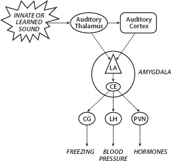
FIGURE 1. Auditory Amygdala Stimuli and Defense Responses. Source: LeDoux (2002, Figure 5.6)

Wiring: The Amygdala in a Nutshell⁴⁵

As LeDoux writes, “The basic wiring plan is simple: it involves the synaptic delivery of information about the outside world to the amygdala, and the control of responses that act back on the world by synaptic outputs of the amygdala. If the amygdala detects something dangerous by its inputs (discussed further below) then its outputs are engaged. The result is freezing, changes in blood pressure and heart rate, release of hormones, and lots of other responses that are either preprogrammed ways of dealing with danger or are aspects of body physiology that support defensive behaviors.” (LeDoux, 2002, pp. 8–9). A simple depiction is given in Figure 1 for an auditory threat stimulus.

Having classified an auditory stimulus as threatening (innately or through conditioning), the auditory thalamus projects (emits an action potential) to the lateral amygdala (LA) and auditory cortex, which also projects a more refined signal to the LA. The central amygdala (CE) then activates various systems to produce responses, such as those shown: freezing, increases in blood pressure, and the release of various hormones. (Further responses are discussed later.)

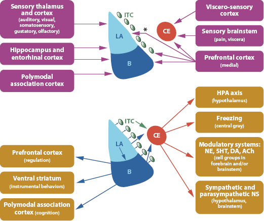
FIGURE 2. Amygdala Inputs and Outputs. Inputs to some specific amygdala nuclei. Asterisk (*) denotes species difference in connectivity. (Bottom) Outputs of some specific amygdala nuclei. 5HT, serotonin; Ach, acetylcholine; B, basal nucleus; CE, central nucleus; DA, dopamine; ITC, intercalated cells; LA, lateral nucleus; NE, norepinephrine; NS, nervous system. Source: Rodrigues, LeDoux, and Sapolsky (2009)

In somewhat greater detail, the neural mechanism of amygdala inputs and activation, and amygdala output, are conveyed in the diagrams of Figure 2. Inputs are depicted in the top, and outputs are shown in the bottom diagram (Figure 2).

The blue almond-shaped structure here corresponds to stunning micrographs of stained brain slices like the one shown below in Figure 3 (LeDoux, 2008).

One essential point is that this architecture supports a critical delay between unconscious and conscious responses to stimuli.

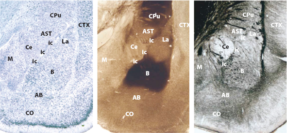
FIGURE 3. Key Areas of the Amygdala. Key areas of the amygdala, as shown in the rat brain. The same nuclei are present in primates, including humans. Different staining methods show amygdala nuclei from different perspectives. Left panel: Nissl cell body stain. Middle panel: acetylcholinesterase stain. Right panel: silver fiber stain. Abbreviations of amygdala areas: AB, accessory basal; B, basal nucleus; Ce, central nucleus; itc, intercalated cells; La, lateral nucleus; M, medial nucleus; CO, cortical nucleus. Non-amygdala areas: AST, amygdalo-striatal transition area; CPu, caudate putamen; CTX, cortex. Source: LeDoux (2008, p. 2698); reprinted courtesy of Joseph E. LeDoux

Inputs: High Road and Low Road

For example, “auditory inputs reach the lateral amygdala⁴⁶ from the auditory thalamus and auditory cortex … These provide a rapid but imprecise auditory signal to the amygdala. Cortical inputs from the auditory and other sensory systems … provide the amygdala with a more elaborate representation than could come from the thalamic inputs. However, because additional synaptic connections are involved, transmission is slower” (Ledoux, 2007). Hence, LeDoux (2002) calls these “the low road and the high road,” as depicted in Figure 4.

I instantly freeze at the snake (low road) but then evaluate it as being a benign garter snake (high road), not a true black mamba, for instance. While the extreme rapidity of the unconscious response is of immense evolutionary value, we will see that, from a social standpoint, the lag between it and conscious appraisal is a decidedly mixed blessing.

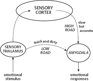
FIGURE 4. Low Road and High Road to Fear. Source: LeDoux (2002, pp. 61–63, Figure 5.7)

Outputs

Continuing, “once the amygdala detects a threat, its outputs lead to the activation of a variety of target areas that control both behavioral and physiological responses designed to address the threat,” (Rodrigues, LeDoux, and Sapolsky, 2009, p. 294). Beyond freezing, amygdala activation induces the release of numerous neurotransmitters (e.g., serotonin and dopamine), increasing arousal and vigilance. Endocrine and autonomic responses are also dramatic, “including increased blood pressure and heart rate, diverting stored energy to exercising muscle, and inhibiting digestion” (Rodrigues, LeDoux, and Sapolsky, 2009, p. 295).

The pupils dilate to allow more light to enter. The heart rate picks up, and the heart muscle contracts more strongly, driving more blood to the muscles. Contractions of selected vascular channels shift blood away from the skin and intestinal organs toward the muscles and the brain. Motility of the gastrointestinal system decreases, and digestive processes slow down. The muscles along the air passages of the lungs relax, and respiratory rate increases, allowing more air to be moved in and out. Liver and fat cells are activated to furnish more glucose and fatty acids—the body’s high-energy fuels—and the pancreas is instructed to release less insulin. The reduction in insulin allows the brain to draw off a sizeable fraction of the glucose entering the bloodstream because, unlike other organs, the brain does not require insulin in order to utilize blood glucose. The neurotransmitter that triggers all these changes is norepinephrine (Bloom, Lazerson and Nelson, 2001, p. 172).

For wonderful discussions, see also Darwin’s The Expression of Emotions in Man and Animals (1872).⁴⁷ Contemporary scientific publications present these input-output (and additional feedback) pathways in various levels of detail. Highly detailed is LeDoux (2007).

On the experience, or “feeling,” of fear, Öhman and Wiens (2003, p. 270) paraphrase LeDoux (1996):

The fear module is primitive in the sense that it was assembled by evolutionary contingencies hundreds of millions of years ago to serve in brains with little cortices. However, it now operates in a human brain capable of advanced thought, language, and the conscious experience of emotion. Humans can talk about emotions, and they have emotional experiences. Awareness of an emotion not only depends on the recognition of an emotional stimulus but also originates primarily in feedback from the emotional responses that are elicited by the stimulus. For example, experiencing a racing heart when a shadow appears from a dark alley contributes to the feeling of fear. In fact, in perhaps the most classic of all classical contributions to the psychology of emotion, William James (1884) proposed that such feedback is the emotion. To paraphrase, you feel the emotion when you experience its effect on your body. Thus the feeling of fear is the experience of an activated fear module.

Current research on the neurophysiology of fear shows James to have been remarkably prescient, despite lacking any modern tools. Very importantly, from a social standpoint, the fear circuit can be activated, and fear conditioning can occur, unconsciously.

Unconscious Activation and Conditioning

In humans, “the fear module can be activated, and fear conditioning can occur without our conscious awareness.” Indeed we need not ever become conscious of it. As LeDoux continues, “… unconscious operation of the brain is the rule rather than the exception throughout the evolutionary history of the animal kingdom. … And this, moreover, confers a selective advantage … if we had to consciously plan every muscle contraction our brain would be so busy we would probably never end up actually taking a step or uttering a sentence” (LeDoux, 2002, p. 11). Among the many demonstrations that amygdala activation per se need not be conscious, the so-called backward masking experiments are particularly elegant.

In backward masking, “an emotionally arousing visual stimulus is flashed on a screen very briefly (a few milliseconds) and is then followed immediately by some neutral stimulus that stays on the screen for several seconds. The second stimulus blanks out the first, preventing it from entering conscious awareness (by preventing it from entering working memory)” (LeDoux 2002). But the first still elicits the full suite of physiological responses—increased heart rate, blood pressure, sweaty palms, and so forth. “Since the stimulus never reaches awareness (because it is blocked from working memory), the response must be based on the unconscious processing of the stimulus rather than on conscious experience of it. By short-circuiting the stages necessary for the stimulus to reach consciousness, the masking procedure reveals processes that go on outside of consciousness in the human brain” (LeDoux, 2002, p. 208). In short, the stimulus makes it to the amygdala by the quick and dirty “low road,” but its arrival in working memory (the high road) never occurs. Cacioppo et al. (2007) write, “The amygdala is particularly sensitive to fear faces (Adolphs et al., 1999; Breiter et al., 1996) even when they are presented so rapidly as to not be consciously perceived (Morris, Öhman, and Dolan, 1999; Whalen et al., 1998). For another nice discussion of backward masking, see Penrose, 1999.⁴⁸

As recent evidence of our capacity for unconscious conditioning proper, a very interesting study by Arzi et al. (2012) demonstrates that associative learning can occur even while we are asleep.

Delayed Feelings

If we do become conscious of fear-inducing stimuli, moreover, we may do so only after the physiological responses. Only after we have ducked from the darting bat do we notice that our heart is pounding, and we ask, “Whoa, what the heck was that!?” The conscious experience of fear, in other words, is a brain state induced by the unconscious activation of neurophysiological precursors driven by the amygdaloid complex (LeDoux, 2002, p. 208). Or, to paraphrase William James (1884), We don’t run because we fear the bear. We fear the bear because we run.⁴⁹

Adaptive Innate Capacity

A range of stimuli will elicit this unconscious activation—we instinctively crouch protectively at unexpected explosions nearby or when unexpected projectiles dart at our heads. In other words, certain sensory inputs will innately generate the threat response. In rats, for example, cats are in this set of innate threats. In fact, rats bred in colonies completely isolated from cats for many generations will freeze upon first exposure to cat urine (LeDoux, 2002, p. 4).

Notice, however, that animals equipped only with a fixed set of specific threats would be vulnerable to novel ones. So, it would be advantageous if the set could be expanded to include novel threats. And it obviously can. Pleistocene man never encountered a BMW, but we freeze when a car whips around the corner at us, just as he froze when huge animals charged suddenly from the tall brush. We are harnessing the same innate fear-acquisition capacity—the same innate neurochemical computing architecture. Miraculously, synaptic plasticity permits us to adapt the evolved machinery to encode novel threats. Detailed neurochemical accounts are given in LeDoux (2002, pp. 89–90).

Retention

There is little point is learning to fear hippos on Monday and then forgetting to on Tuesday. So, the retention of acquired fear associations is obviously essential in such cases and is achieved by various forms of long-term potentiation (LTP) at the synaptic level. This is also becoming understood neurochemically and is treated in Bauer, Schafe, and LeDoux (2002). Like unconscious fear acquisition, this fear retention is also significant socially, as we will discuss later in connection with “extinction.”

Observational Acquisition

Finally, it would also be advantageous if one could condition on the aversive experience of others—if you could acquire fear of the red-hot stove by watching me get burned, without having to get burned yourself. As we will review, this too is possible. Indeed, so-called mirror neurons may have evolved for this very purpose (see the discussion on p. 62). The result is that fear is, in a defensible sense, contagious (Hatfield, Cacioppo, and Rapson, 1994). This will be further discussed shortly.

All in all, then, as LeDoux observes, “It is a wonderfully efficient way of doing things. …” Rather than create a separate system to encode each new danger, “just enable the [single] system that is already evolutionarily wired to detect danger to be modifiable by experience. The brain can, as a result, deal with novel dangers. … All it has to do is create a synaptic substitution whereby the new stimulus can enter the circuits that the pre-wired ones used” (LeDoux, 2002, pp. 6–7).

Perils of Fitness

It is indeed a most wonderful machinery. But it is also terrible: it makes us deeply vulnerable to the unconscious construction and retention of racial, ethnic, and other fears and biases [on race, LeDoux (2003); Telzer et al. (2012); on racial face masking, Öhman (2005)]. It predisposes us to rash, often violent, overreactions and opens us to all manner of nefarious manipulation. Indeed, fear conditioning has been a fundamental tool in most propaganda since time immemorial.⁵⁰ But, equally disturbing, fear can spread in a completely decentralized manner, propelling mass violence, financial crises, and deeply misguided health behaviors for example. See LeDoux (2002, p. 124):

As Pavlov suspected, defense conditioning plays an important role in the everyday life of people and other animals. It occurs quickly (one pairing of the neutral and aversive stimulus is often sufficient) and endures (possibly for a lifetime.) These features have no doubt become part of the brain’s circuitry due to the fact that an animal usually does not have the opportunity to learn about predators over the course of many experiences. If an animal is lucky enough to survive one dangerous encounter, its brain should store as much about the experience as possible, and this learning should not decay over time, since a predator will always be a predator. In modern life we sometimes suffer from the exquisite operation of this system, since it is difficult to get rid of this kind of conditioning once it is no longer applicable to our lives, and we sometimes become conditioned to fear things that are in fact harmless. Evolution’s wisdom sometimes comes at a cost.” [Emphasis added.]

In other words, fitness is perilous: the innate fear module is double edged. The self-same rapid-fire, unconscious, nondeliberative fear-association machinery that allowed us to avoid predators on the African savannah leaves us profoundly vulnerable to manipulation, to unreflective acquisition of biases, and to being swept up in mass hysterias from Salem witches to genocides to the run on banks that precipitated the Great Depression.

Know Thyself

Self-knowledge (and self-control) requires that we recognize these powerfully evolved forces. Denying their existence simply increases our vulnerability to them and to their manipulation. That we possess this fear-conditioning apparatus is beyond reasonable dispute. This, however, is emphatically not to say that human behavior is determined by conditioning. First, the capacity to extinguish conditioned fear is also part of the innate human endowment, is also backed by overwhelming experimental evidence, and is also being mapped neurochemically. This is discussed later under the topic of extinction. But, beyond that, a central point of the present model is that unconscious conditioned fear may be modified both by conscious deliberation and (often unconscious) social influence. This is not to say that the overall outcome is necessarily “better than” the purely fear-inspired one; only that, as a scientific matter, (a) conditioning can be transitory and (b) much beyond conditioning is going on. Fear conditioning is incontrovertibly a part of the human condition (pun intended), and it is part of my model, along with much else.

Nomenclature of Conditioning

With all this as background, we review some standard nomenclature adopted by Pavlov in his monumental study, Conditioned Reflexes: An Investigation of the Physiological Activity of the Cerebral Cortex.⁵¹ This terminology is necessary to present the Rescorla-Wagner model. To begin, the following are now standard definitions.⁵²

Definitions

US: unconditioned stimulus [food]

UR: unconditioned response [food-induced salivation]

CS: conditioned stimulus [bell]

CR: conditioned response [bell-induced salivation]

Initialize

CS (bell) alone → 0 (no response)

US (food) alone → S (salivation)

Associative Learning

CS–US pairing trials: bell/food, b/f, b/f, …

When Conditioned:

B alone → S … CR = UR

The US is called unconditioned because no conditioning is required for it to elicit the response. For Pavlov’s dog, food (US) induces⁵³ salivation without any conditioning. Hence salivation is termed the unconditioned response (UR). The conditioned stimulus (CS), by contrast, initially elicits nothing. Pavlov (1903) actually repeated his experiments with a number of different conditioning stimuli, including the famous bell. Through repeated pairings with the US, the CS acquires salience and eventually alone elicits a response, called, naturally, the conditioned response (CR). Because it emerges through repeated associations of the US and the CS, the conditioning process is also called associative learning.

Hume’s “Association of Ideas”

Although a synaptic account of this process would require another 300 years of research, Hume recognized the general phenomenon of conditioned association, and even saw this as his signal contribution.⁵⁴ In An Enquiry Concerning Human Understanding (1748; 2008 ed., pp. 106–7), he writes “… after the constant conjunction of two objects … we are determined by custom alone to expect the one from the appearance of the other … Having found in many instances, that two kinds of objects—flame and heat, snow and cold—have always been conjoined together; if flame or snow be presented anew to the senses, the mind is carried by custom to expect heat or cold.” It is not by reasoning, moreover, that we form the connection. “All these operations are a species of natural instinct, which no reasoning or process of the thought and understanding is able either to produce or to prevent” (Section V, Part I).

Hume even recognized the benefit (though perhaps not the cost) of a lag between reflexive response (low road) and deliberation (high road). He writes that, since this innate associative capacity

is so essential to the subsistence of all human creatures, it is not probable that it could be entrusted to the fallacious deductions of our reason, which is slow in its operations; appears not in any degree in infancy;⁵⁵ and at best is, in every age and period of human life, extremely liable to error and mistake. It is more conformable to the ordinary wisdom of nature to secure so necessary an act of the mind, by some sort of instinct or mechanical tendency, which may be infallible in its operations, may discover itself at the first appearance of life and thought, and may be independent of all the laboured deductions of the understanding [emphases added] (Section V, Part I).

It is difficult to fathom so modern a perspective from someone born (in 1711) a century before Darwin (b. 1809), who would discover that Hume’s “ordinary wisdom of nature” is none other than natural selection. Through the researches of Pavlov, de Cajal, Hodgkins and Huxley, and many others, we now do know something of the “mechanical tendency” Hume intuited. But it was only in the mid-20^th century that mathematical models of condi-tioning emerge.

En route to a very famous one of these, modern nomenclature uses V for the Associative Strength of the CS and US. It is the extent to which the CS (the Bell) elicits the UR (salivation), or, equivalently, it is the proximity of the CR to the UR.⁵⁶ Obviously, V changes over time, with repeated pairings, and in a manner usefully captured by the Rescorla-Wagner equations (to be presented shortly).

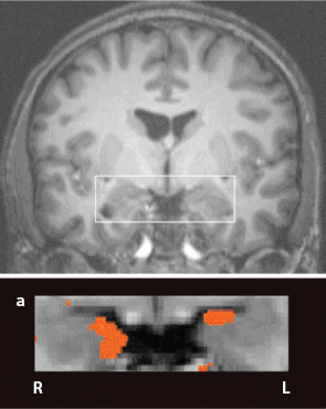
FIGURE 5. Postconditioning Amygdala fMRI. Source: Reprinted by permission from Macmillan Publishers Ltd: Nature Neuroscience (Olsson and Phelps 2007, p. 289), copyright 2007

One exemplary experiment (Olsson and Phelps, 2007) uses color as the CS, electric shock as the US, and repeated color-shock conditioning trials. After a number of these color-shock pairings, the associative strength (V) of color and shock is sufficiently great that the color (the CS) alone elicits the anticipatory shock fear, measured by conductive skin response (CSR) and by functional magnetic resonance imaging (fMRI). The fMRI image in Figure 5 shows the (blood-oxygenation-level-dependent) BOLD signal in the subject’s amygdala on presentation of the CS after fear conditioning. This will prove to be of central interest below.

All brain imagery needs to be interpreted with great care (Vul et al., 2009a, b). A black-lung X-ray does not depict the feeling of respiratory distress and this fMRI does not depict the feeling of fear. But someone with a black-lung X-ray will almost certainly have trouble breathing. In medicine, feelings are symptoms. The instrumental readouts are signs. But signs are often correlated with symptoms, and that is my basic presumption here. There are many and varied correlates of fear, as reviewed earlier. Amygdala activation is a central neural one.⁵⁷

Theory of Conditioning

There is a basic mathematical theory of the conditioning process that we shall adopt, recognizing that numerous refinements and extensions are possible. These are high-level—low-dimensional—equations developed in 1972 by Rescorla and Wagner. They do not represent the neural level at all. Their fidelity is explained by the contemporary neuroscience. They are analogous to the Kermack-McKendrick disease-transmission model (Kermack and McKendrick, 1927), which gives a very useful account of disease transmission through well-mixed populations without representing the microbiological interaction of pathogen and host immune systems, which, of course, explains transmission. From a neuroscience perspective, the Rescorla-Wagner model is a highly aggregate relationship describing an associative process generated by Hebbian plasticity at the synaptic level. It is a summary relationship explained by physicochemical synaptic interactions, which are quite well understood. So, here we are representing gross fear-learning dynamics that are explained by a lower neural level. For our social science objectives, this is a suitable modeling resolution.

The Rescorla-Wagner Model

The Rescorla-Wagner model (1972) is a cornerstone in the mathematical theory of conditioning and will form the basis for Agent_Zero’s emotional module.⁵⁸ Though I will generalize it slightly to accommodate a broader range of conditioning trajectories, for present purposes, Rescorla-Wagner works nicely. It is

Exposition

Imagining a fear-conditioning exercise of the sort discussed before, let t index the paired presentations of the US and CS. So t = 1 is the time of first pairing; t = 2 is the time of second, and so forth. (One could assume that trials are a Poisson arrivals process, for example. Here, we assume these are equally spaced and identical in duration and all other respects). At each pairing there is some associative strength between the CS and the US—some degree to which the CS alone elicits (i.e., the CR approximates) the UR—for instance, the extent to which the bell alone (CS) elicits the salivation (in milliliters) normally elicited with no conditioning by food (the US). This is the value of v_t, the associative strength at trial t.⁵⁹ The pretraining association is v₀ and could be positive but will here be zero. Before any training, in other words, the bell alone elicits no salivation.

The Rescorla-Wagner model concerns the change in associative strength as trials proceed. The left-hand side is the difference between v_t+1 and v_t. If we, advisedly, use the loaded term learning to denote this difference, we can coherently ask the question, When does learning stop? It stops when the left-hand side equals zero—when there is no change between v_t and v_t+1. The right-hand side must also equal zero, which occurs when v_t reaches the value λ, since α and β are constants (to be discussed shortly). Hence, λ represents the maximum associative strength attainable in the training process of interest and might also have been denoted v_max. So, if the association is already at capacity, no further gain in association is possible. Hence, the difference between λ and v_t is interpreted as surprise (This is sometimes referred to as the subject’s prediction error). Once the associative strength of chocolate and sweetness is unity, we are not surprised when chocolate is, in fact, sweet. But our first taste of chocolate is pleasantly surprising. Finally α and β are nonnegative constants representing the salience of the CS and the salience of the US, respectively. They are often termed learning rates. High surprise and salience can produce very rapid conditioning. For Little Albert—recalling James Watson’s infamous experiment of the 1920s—the clang of a hammer on a metal bar (the US) is salient and highly aversive, while the little furry white mouse (the CS) is initially salient and snuggly.⁶⁰ It is shocking to the infant Albert that the two would be associated so—with Watson’s repeated pairings of the clang and the mouse—little Albert “learns” quickly to fear the mouse. Albert, in fact, generalized this to fear all furry animals. If either the mouse or clang had lacked salience, he might have had a pet rabbit (no aversive association would have been formed).

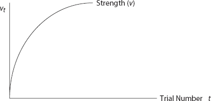
FIGURE 6. Rescorla-Wagner Associative Strength Trajectory

Observe that with, α and β positive and v increases with each trial, but at a decreasing rate, approaching λ asymptotically. Learning—the change in association—is greatest at the outset, declining as the maximum association is approached,⁶¹ as shown in Figure 6.

Unless otherwise stipulated, the variable, t, will denote trials. The Rescorla-Wagner model is a first-order initial value nonhomogeneous linear difference equation and is solvable analytically. To wit,

whose solution is:

The asymptotic value of v is λ, as it should be (that is, ). Now, analytical solution in hand, we can begin to ask a number of interesting questions about our disposition model.

Tipping Point

For example, assuming the preceding affective trajectory, at what trial will the individual “tip” into taking action? In the model (without deliberative or social modules yet), this occurs when v_t > τ, the action threshold, as shown in Figure 7.

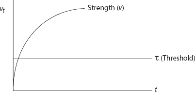
FIGURE 7. Rescorla-Wagner Trajectory and Threshold

Using the general solution, this is equivalently

We solve for the threshold time:⁶²

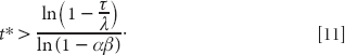
This makes good sense. Increasing the threshold delays the tipping. If either α or β is zero, tipping never occurs since

meaning that if both stimuli (CS and US) lack all salience, the action is never tripped.

For completeness sake, and because we will employ it below, the differential equation (as against the difference equation) version of the Rescorla-Wagner model is

With v(0) = 0, the solution is

The central point of the Rescorla-Wagner model, in either form, is that high surprise combined with high salience produces strong associative conditioning. To anticipate slightly, another distinctive feature is that conditioning depends on the aggregate stimulus, the sum of the v_i’s—the associative strengths taken over all stimuli—a point to which we will return.

Once again, the model does not assume that people are aware of these affective dynamics. Indeed, a central point of the preceding discussion is that, typically, they are not (Phelps in Lewis, Haviland-Jones, and Barrett, 2008, p. 236; LeDoux, 2002). We may not be conscious of our conditioning (i.e., the reduction in prediction error λ − v) even if we are conscious of the CS-US pairings. And, in backward masking, even these are not registered.

Social Examples

We are well acquainted with conditioning trials in which the CS is a bell, the US is food, and the CR is salivation or where the CS is a light, the US is a shock, and the CR is fear. But, there is every reason to postulate analogous patterns of profound social consequence, as suggested in Table 1. It is surprising and profoundly salient when an unfamiliar social group attacks others, or when a trust is betrayed. Associations born of shocking and salient social events can elicit extremely strong reactions, as suggested in Table 1.⁶³

Recognizing the model’s generality, let us focus on one of our social examples. The September 11, 2001, World Trade Center attacks were surprising and salient. One could argue that there were four primary conditioning trials, one for each tower plus one for the Pentagon attack and one for Pennsylvania flight 93. In fact, there were countless further exposures in the form of video replays of the aircraft impacts and subsequent collapse of towers, people leaping from buildings, terrified flight, and other images. The unconditioned response (UR) was fear and intense anger toward the perpetrators. The conditioned stimulus (CS) was the face of Osama Bin Laden or Mohammed Atta—the “Arab face,” as it were.

TABLE 1. Surprise, Salience, and Conditioning

CS	US	UR/CR
Light	Shock	Fear
Japanese face	Pearl Harbor	Rage/internment
Arab face	9/11	Rage/internment
Vaccine	Report of adverse reaction	Fear/vaccine refusal
Doctor	Tuskegee	Enduring distrust
Asset	Collapse	Dumping

The resulting associative strength was extremely high, as expected on good Rescorla-Wagner (RW) grounds.⁶⁴ Most Americans had little prior exposure to Muslims and certainly had never heard the phrase “Al Qaeda” before, so there was no damping of the association by prior conditioning. And, as expected, we saw rapid “learning,” in the RW sense. After the four direct trials and countless reexposures in all media, the average CR to symbols of the Muslim world (CSs) was very high up the learning curve.

“A comprehensive LexisNexis database survey of U.S. newspaper reports between September 1 and October 11, 2001, found an increase in hate crimes toward persons believed to be of Middle Eastern descent (from 1 to 100 events involving 128 victims and 171 perpetrators) across 26 states” (Swahn et al., 2003; Marshall et al., 2007, p. 311). Fourteen of these were murders. “Most [attacks] occurred within the period 10 days after the 9/11 attacks” (p. 311).

Remarkably, “only 42% of the victims were of Middle Eastern descent,” the remaining attacks being “against persons of color who are perceived to be vaguely reminiscent of the 9/11 terrorists” (Marshall et al., p. 311). Even a very broad and vague attribute (general skin hue) can serve as a CS. This is an example of stimulus overgeneralization, where subjects conditioned on a particular CS—an 800-hz tone—will respond to a very rough approximation of it (e.g., a 1000-hz tone).

Olsson and Öhman (2009, p. 736) write, “For example, there are now numerous demonstrations that unknown racial outgroup members, that is, individuals not belonging to one’s own racial group, can elicit a rapid threat response associated with the amygdala” (Cunningham et al., 2004; Phelps et al., 2000). They even speak of “the possibility of a hard-wired disposition to develop xenophobic responses” (p. 736). This is not to say that xenophobia itself is inevitable. Indeed, they also note that out-group dating experiences can nullify the effect. Why this in-group bias might have evolved is modeled in Hammond and Axelrod (2006a, b). The first fMRI study of prejudice was Hart et al. (2000; see also Cunningham & Van Bavel, 2009, p. 978).

Blocking and Selective Discrimination

Relatedly, I find it very revealing that the Japanese were the only ethnic group interned on a mass scale by the United States during WWII, even after 1944, when the United States was fully at war with Germany and Italy. In 1939, The German-American Bund had staged a 20,000-person pro-Nazi rally in New York’s Madison Square Garden. The Bund ran a dozen youth camps in various states and published eight newspapers. Once the United States entered the war, the Bund was banned, but, unlike the Japanese (who had never organized anything comparable), few German-Americans were interned. Even fewer Italian Americans were interned, despite fascist Italy’s alliance with Hitler. Beyond the unique scale of their internment, the Japanese were distinctive in that more than 60% of those interned were, in fact, American citizens.⁶⁵

This, too, is entirely consistent with the general version of the Rescorla-Wagner model, in which the total associative strength v^TOT is distributed over the sum of all conditioning stimuli of relevance. If we let stand for the associative load on the Japanese at time t, and the load on European axis powers, the total strength is given by⁶⁶

If the associative strength of is already close to λ, there is very little associative capacity left for In these terms, the associative load on the Japanese face was so large after Pearl Harbor (shocking and salient) and the ensuing war in the Pacific as to “block” a comparable association on Aryan features or Italian accents.

Interestingly, very few Japanese in Hawaii were interned.⁶⁷ It could be that they were grudgingly tolerated as essential to American naval base operations. But one could also explain this by Rescorla-Wagner: Japanese people were part of the fabric of Hawaiian society, composing a third of the population. Non–Japanese Americans living in Hawaii had accumulated sufficient positive experience (prior exposure) as to “block” the level of fear that continental Americans associated with the (far less familiar) Japanese after Pearl Harbor. Analogously, on 9/11, most Americans had no such prior exposure to Muslims, and no blocking of the maximal associative load occurred. The phenomenon of blocking has been studied extensively, beginning with the classic paper of Kamin (1969).

Betrayals Real and Imagined

Betrayals of trust are often very surprising and salient. The Rescorla-Wagner model may explain why they generally loom so large in human memory. The betrayal of trusting black Americans by the medical establishment at Tuskegee is a stark example. It was very surprising and highly salient. It actually continued until 1972 and so is a deep trauma well within the memory of black Americans today. Judas betrays Christ; Brutus betrays Caesar; Greek mythology is rife with betrayals (Clytemnestra betrays Agamemnon); “Uncle” Joe Stalin (ally in WWII) betrays the war allies by occupying Eastern Europe; the Jews allegedly “stabbed Germany in the back” after WWI.⁶⁸ Benedict Arnold betrays the colonies. They are instances of highly salient surprise. The “revelation” of betrayal by conspiracies is a trusted tactic among fear mongers to this day. See Richard Hofstadter’s (1964) wonderful essay, “The Paranoid Style in American Politics.”⁶⁹

By the same token, some salient surprises are reserved for occasions meant to elicit a burst of strong and happy associative strength—like marriage proposals. Many expectant parents choose not to learn the sex of their children till birth, preserving a highly salient surprise.

So, here we have our first building block of Agent_Zero—Rescorla and Wagner’s very elegant model of conditioning. We understand that this is an aggregate relation that is ultimately explained by the neuroscience, which licenses us to interpret the model as unconscious fear acquisition harnessing the same Pleistocene apparatus that got us here,⁷⁰ a neurophysical apparatus that was reviewed in some detail.

Now, as noted, a number of factors can militate against our blind submission to unconscious fear impulses. Counterevidence is one; peer pressure is another. These will both be further building blocks added to the model. But, even within the Rescorla-Wagner framework, there is allowance for the fading of fear.

Fear Extinction

Our synapses are plastic, and so are we—we can learn, and we can unlearn (Rescorla and Wagner, 1972). Conditioned associations are not necessarily permanent and often decay if pairing trails cease. This is called extinction,⁷¹ a term introduced by Pavlov. In the Rescorla-Wagner (RW) model, the extinction phase is handled very elegantly simply by setting λ, the limiting value of v, to zero (since all association is to die out), and the initial value of v to whatever value it had attained immediately when conditioning trials are terminated; let us denote this latter value v_max. In differential equation form (moving freely between discrete and continuous time), associative strength thus diminishes according to

The solution is the well-known formula for exponential decay,

Overall, then, the conditioning and extinction phases of an RW process are not symmetrical, and most likely involve different brain regions [as discussed shortly]. Conditioning is increasing and concave down, with an upper asymptote of λ. Extinction is decreasing and concave up, with an asymptote of zero. When conjoined the acquisition and extinction phases have a distinctive shape, with an abrupt change in concavity at the (nondifferentiable) acquisition-extinction transition point, as shown in Figure 8.⁷²

General Solution of the Two-Phased Model

Typically, the two phases (acquisition and extinction) are solved and discussed separately. I have not seen it observed that the entire two-phased model can be expressed using Heaviside unit step functions.⁷³ With t* the time at which trials cease, the full solution is then

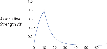
FIGURE 8. Acquisition and Extinction

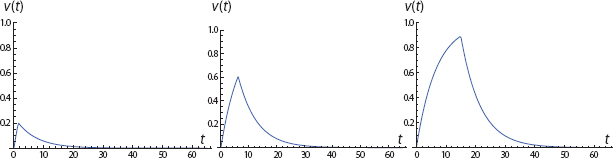
FIGURE 9. Final Acquisition Level and Initial Extinction Rate

This gives the entire learning and extinction trajectory. A movie of the entire acquisition and extinction history, as parameters are varied, is given as Animation 0 on the book’s Princeton University Press Website.⁷⁴

An impressive property of the two-phased model is that the (negative) extinction slope increases in magnitude with the terminal phase 1 conditioning level, as noted in the panels of Figure 9. The greater the acquisition level, the greater (i.e., steeper) the initial extinction rate.⁷⁵

The curious asymmetry of the model makes its extensive corroboration all the more impressive. Countless experiments with animals, including humans, have conformed to this basic relationship. For example, conditioning trials with humans exhibit the same qualitative profile as the following rat trials (Figure 10).

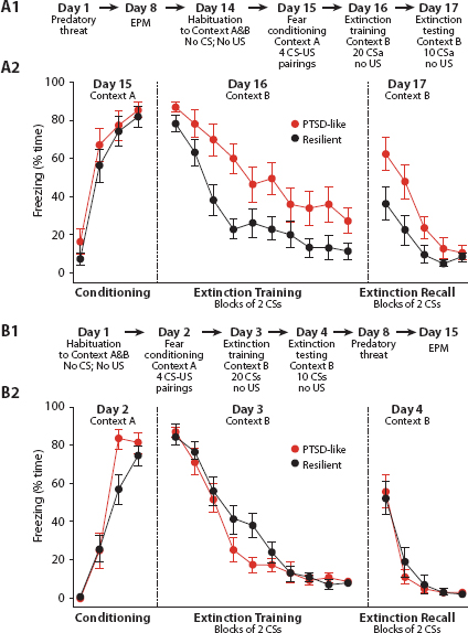
FIGURE 10. Acquisition and Extinction of Conditioned Fear Response for Predatory Threat. Source: Goswami et al (2010, p. 496)

Moreover, there are strong arguments as to why the animal models are reasonable predictors of human fear conditioning behavior (Bloom, Lazerson, and Nelson, 2001). Obviously, we do not fear what the rat fears, but we fear how the rat fears.⁷⁶ The same neuroanatomy and cellular-synaptic mechanisms have been preserved across vertebrate evolution. LeDoux calls these conserved structures “survival circuits.” In his most recent terminology, the fear circuitry we’ve reviewed is cast as an instantiation of these. For a full account see LeDoux (2012). A compendious review of the human conditioning literature is Sehlmeyer et al. (2009).

Although the Rescorla-Wagner model has been refined in Pearce and Hall (1980), Sutton and Barto (1998), and other descendants, the classic model deserves the status of other canonical models—the Kermack-McKendrick model of infectious disease; the Lotka-Volterra model of predatorprey cycles, the Richardson arms-race model, and so forth. Like fundamental models in many fields, it elegantly offers important insight and explains a wide range of observed phenomena.⁷⁷ It is a revealing simple model.

Affective Persistence: The Half-Life of Hatred

Because extinction is seldom immediate, affect (positive or negative) can remain above the action threshold long after the stimulus has stopped. Cycling back to our social examples, then, anti-Japanese sentiment generally continued beyond the war. The informal Jewish boycott of German goods persisted (indeed persists) long after WWII. As public health examples, the scars of Tuskegee still affect minority trust of the U.S. public health establishment (Corbie-Smith, Thomas, and St. George, 2002; Freimuth et al., 2001). Such distrust is evident in The Pittsburgh Barbershop study (Using Social Norms to Attack Prostate Cancer among African Americans, National Center on Minority Health and Health Disparities), in survey results on smallpox vaccine refusal (Lasker, 2004), and in the Washington, D.C. postal workers’ cipro (ciprofloxacin) refusal after the anthrax attacks of 2001(Quinn, Thomas, and Kumar, 2008; Quinn, Thomas, and McAllister, 2005). The last example is stark in that predominantly white Congressional staff were eager for cipro. The same general pattern occurred with H1N1 (swine flu) vaccine in 2009, despite the swine flu being declared a global pandemic by the World Health Organization.

Fear conditioning and the extinction of fear, in other words, are not symmetrical, a point made nicely by the Rescorla-Wagner model. It is amazing that seemingly remote processes can share the same mathematical description [e.g., the wave equation; see J. M. Epstein (1997)]. Even in social science, a huge number of social situations have the form of a Prisoners’ Dilemma, or a Coordination Game.⁷⁸ Here also, the extinction phase of Rescorla-Wagner is formally the same as radioactive decay. So, just as we could compute the tipping point earlier, let us compute the “half-life” of hatred, if you will. The half-life is, by definition, the time at which half the original “substance,” v_max, is gone. It is the time at which

An interesting property of exponential decay is that the half-life is independent of the initial level, as in this case, where the v_max’s cancel out.

Accordingly, logging both sides, we obtain

which is to say that the half-life is

This makes basic sense in that the smaller the decay rate (αβ), the greater the half-life (i.e., the longer it takes until half the initial stuff is gone).

Posttraumatic Persistence

Of course, the mere cessation of conditioning trials is not always sufficient to “reset lambda to zero” and induce the exponential extinction of fear. As LeDoux and Phelps write, “It is important to note … that the extinction of conditioned fear responses is not a passive forgetting of the CS-US association, but an active process, often involving a new learning” (LeDoux and Phelps, 2008, p. 164). In fact, acquisition and extinction of fear may be controlled by different regions—acquisition by the amygdala, and extinction by the ante-rior cingulate of the medial prefrontal cortex (mPFC). A 2005 PET study of women with PTSD resulting from childhood sexual abuse revealed “decreased function or failure of activation in mPFC during fear extinction, in women with abuse-related PTSD compared with controls” (Bremner et al., 2005).

Again, we are not modeling brain regions, but in modeling terms, we have license to say that λ doesn’t necessarily reset to zero when conditioning trials cease (simply because genocidal violence stops, for example).⁷⁹ Below, we exercise this license mathematically (see Figure 33) and show that a single agent’s PTSD can retard the recovery of the entire group. Then, in the agent-based model of Part II, we (I believe for the first time) “lesion” an agent—excising her “software amygdala”—and show the group-level effects.

The Rescorla-Wagner model will be generalized in several ways below. But it will form the backbone of Agent_Zero’s affective component. We turn now to the cognitive (evidentiary/deliberative/ratiocinative) building block of Agent_Zero, having agreed with Hume and countless others, that reason (not only passion) must play a role in any credible model of people.⁸⁰

I.2. REASON: THE COGNITIVE COMPONENT

However, reason is not here assumed to be perfect, but prone to informational limits and associated biases. There is, of course, a vast literature on bounded rationality since Herbert Simon coined the phrase (see Simon, 1982). One can imagine endowing agents with innumerable sources of error. Well-established and systematic departures from canonical rationality include: representativeness and availability biases, anchoring and adjustment, recency effects, the conjunction fallacy, confusion between frequency and magnitude, baserate neglect, and outright logical confusions, to name a few (see Gilovich, Griffin, and Kahneman, 2002; Kahneman, 2003). To start, however, I need the agents to estimate a probability. Why will this be important? Here is the motivation, as always in the context of our binary disposition model.

Imagine that I am confronted with another person, Mr. K, and the binary issue is whether to attack him or not. And, as per our earlier discussion, with no countervailing forces (e.g., fear of retaliation), I will fight K if my visceral feeling (V) that he is my enemy exceeds my action threshold T. If I feel nothing toward K and the data on him indicate a probability (P) of enmity below T, then I will not attack. Suppose now that my feelings (passion) exceed threshold but that my evidence (reason) does not. Then the emotional and cognitive circuits are giving me conflicting signals.⁸¹ Since, tautologically, I either attack or do not, one of these prevails. Exactly how this happens is not well understood but normally comes under the heading of “executive function,” in which certain regions of the prefrontal cortex (PFC) are centrally implicated. We will return to this.

But, to mathematize this in the simplest conceivable way, the situation just described is depicted in Figure 11.

FIGURE 11. Rivalry

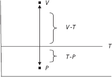
The action threshold is T. Emotion (V) is pulling me upward, urging me to attack. But the evidence (P) suggests I should not. Of course, the action in question could be to pursue an amorous inclination, rather than a violent one, or to flee rather than fight, and so forth. A more colorful rendition of the basic tension is Plato’s allegory of the Charioteer.⁸²

In Phaedrus, Plato depicts man as a Charioteer with two horses, an upward-striving white horse who can lift the Charioteer to the heavenly, reasoned, temperate altitude of the Gods, and a downward-plunging black horse whose wanton animal impulses, if unbridled, will bring the Charioteer crashing to earth.

The black steed can be controlled, but only through great and violent effort. In such moments, the Charioteer, yanking the reins, “falls back like a racer at the barrier, and with a … violent wrench drags the bit out of the teeth of the wild steed and covers his abusive tongue and jaws with blood, and forces his legs and haunches to the ground and punishes him sorely. And when this has happened several times and the villain has ceased from his wanton way, he is tamed and humbled, and follows the will of the Charioteer” (Edman, ed., 1956, p. 297). For Plato, one steed strives upward, and one strives downward. They pull in opposite directions on the same line, as in a tug of war, in contrast to the orthogonalist Hume. Of course, Hobbes accounted the Charioteer’s prospects as grim, arguing that a monolithic Leviathan state is required to bridle, as it were, our warlike impulses, lest ‘the life [of man] be solitary, poor, nasty, brutish, and short” (Hobbes, 1660; 1958 ed.).

Returning to the mathematics, in Figure 11, passion (V) pulls up, but evidence (P) pulls down.⁸³ Oddly, my model says to add them (see equation [1]). Why? Returning to our first example, the argument is that, to attack, V must be pulling up more than P is pulling down—in other words, that V exceeds the threshold by more than the threshold exceeds P, as shown in Figure 11.

Mathematically, this means V − T > T − P, or that

Passion plus reason must exceed twice the threshold, as it were.⁸⁴ So, addition—first introduced in the skeletal equation—is a defensible starting point, but as we see, a further argument can be provided. The sum, moreover, must satisfy a perhaps unexpected relation. Another way to think of this, of course, is that the average, (V + P)/2, must exceed the threshold. Obviously, if V and P are both above (or both below) T there is no rivalry, while in Figure 11, no action is taken (i.e., reason wins) if (V + P)/2 ≤ T.⁸⁵

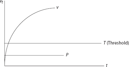
As reviewed before, the Rescorla-Wagner model produces a V-curve, not just the point in Figure 11. So, assuming that P > T, the full dynamic picture is shown in Figure 12. Instead of the point, we now imagine associative strength developing through trials as per the Rescorla-Wagner model. The action threshold remains V + P = 2T, but V is now a curve, not a point. If and when V exceeds 2T − P, Agent_Zero acts (e.g., attacks).

All right, so this is how Agent_Zero’s probability estimate, P, will function in the model; this is how he uses P. But where does Agent_Zero get a value for P?

In the agent-based version of Part II, he computes it from data he collects. The agent model developed there is spatial. Events unfold on a grid of cells. Agents have a spatial sample radius. If this sample radius is 1, they can survey the adjacent cells immediately to the north, south, east, and west, their so-called Von Neumann neighborhood.⁸⁶ If the radius is 2, they can inspect eight cells (two in each of the four directions), and so forth. They collect data through observation of cells within their search radius. For example, if we imagine neighboring cells to be people, and posit that yellow cells are friends and orange cells are enemies, then Agent_Zero’s estimate of the global probability that a randomly chosen person is an enemy is his local (i.e., within radius) relative frequency of orange sites. We will interpret this information radius in a variety of ways later (e.g., size of an investment portfolio, range of vaccines). But one interpretation is the literal sensory perception of events in space and time.

FIGURE 12. Dynamic Rivalry

Sample Selection Error

In general, agents want to know the prevalence of some attribute (orangeness) in the overall population of orange and yellow cells. They estimate this by computing the local relative frequency of orange cells within their spatial sample radius, as discussed earlier. This algorithm produces bias because this color may be clustered in certain regions. Compared to the true global orange frequency, sampling in high-density zones produces upward bias, while sampling in denuded areas produces downward bias. Statistically, this is referred to as sample selection error. Cognitively, it arises from what Tversky and Kahneman (1971) dubbed the representativeness heuristic: the common tendency to “expect the statistics of a sample to closely resemble (or ‘represent‘) the corresponding population parameters, even when the sample is small” (see Tversky and Kahneman, 1971, and Kahneman and Frederick, 2002).

Memory

Now, just as agents can look around in space, they can also look back in time. In the agent-based version of the model, they will have “memory”—they will maintain a list—of recent probability estimates (relative frequencies within their spatial sampling radius). If they have memory m, they carry a list of the m most recent values (dropping memories from more than m periods ago). While the code permits various filters (e.g., the moving median), agents will use the moving average of probability estimates over this memory window as their P value. While they are not Bayesians, they do update their estimates based on new data, and prior estimates have inertia. The essential point is that the agents in this model do not remember everything, and what they do remember is typically biased.

Obviously, human memory is a vast and dynamic field of cognitive neuroscience in its own right (Eichenbaum, 2012) and one over which I make no claim to mastery. Agent-Zero’s idealized memory (her evolving list) will serve as a simple starting point in building an agent who can take in and store information from a dynamic environment and estimate from it a probability that affects disposition and, in turn, action.

Even these seemingly crude modeling assumptions, it should be noted, impute to Agent_Zero considerably more numerical prowess than humans can muster without serious training. Butterworth (1999) argues that the computation of frequencies is very difficult for humans and that base rates are hard to estimate because rates per se are hard, hence suggesting a neurocognitive basis for the robustly observed behavioral regularity of base rate neglect (Kahneman & Tversky, 1973).⁸⁷ Moreover, the storage of numbers beyond subitizing (i.e., remembering four values) is also difficult. We will return to the topics of sample selection bias and memory in the agent model of Part II.

Probability in Agent vs. Mathematical Versions

Summarizing the probability discussion, in the agent version developed shortly, the agents’ P-value (a) is acquired through spatial sampling, (b) is remembered, and (c) is dynamic (i.e., it updates) as the agents’ environment changes and agents move spatially. In short, it changes based on the agent’s experience. For expository purposes, in this purely mathematical section, it will be exogenous and fixed.

So, we now have simple versions of two of our three Agent_Zero ingredients: We have a crude model of affective dynamics (passion) using the Rescorla-Wagner Model (to be generalized later to accommodate S-curve learning); and we have a crude model of bounded rationality—our P-estimate (to be generalized and made dynamic and spatial in the agent-based version to come).

Let us now imagine again that the wriggling snake is thrown in our path. First we have the “low-road” unconscious response reviewed earlier: I freeze in primal terror. But then I notice that this could be a simple disinterested garter snake. I assign some P to that prospect. My ultimate behavior in the snake’s presence—flee or just cut a wide swath and pass by—is neither purely emotional nor purely rational. There is a competition or rivalry between them, in which rationality often operates at a distinct disadvantage. Indeed, Charles Darwin himself was deeply interested in this specific example. He actually tried “without success, to withhold a response to the strike of a poisonous snake behind a protective glass cage in a zoo” (LeDoux, 2002, p. 216).

Recap and Transition

To this point, we have developed two of Agent_Zero’s three components: one affective and one deliberative. But “no man is an island,” as it were, and it is now time to add the social component. Elaborating our snake story, first we freeze (the emotional) and then we calm down, seeing that the snake is likely benign (the cognitive). But, if a crowd of horrified people race by shrieking “snake,” we may abandon our cognitive appraisal and run (the social). We now add a social component.

I.3. THE SOCIAL COMPONENT

The simplest conceivable society is comprised of two people. In Figure 13, the vertical axis is person 1’s disposition, and the horizontal axis is person 2’s. Each has an action threshold, τ₁ and τ₂, respectively, dividing the plane into four regions. In the +/+ region both agents are above threshold, while in the −/+ region only person 2 is, and so on.

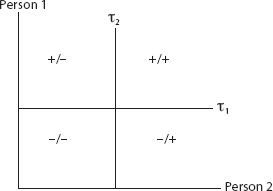
FIGURE 13. Two Thresholds Implies Four Regions

FIGURE 14. Equilibria Benign

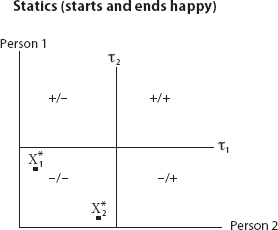
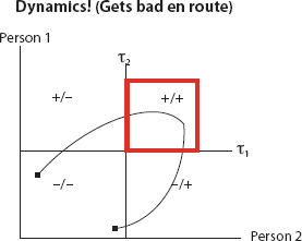
FIGURE 15. Out of Equilibrium

If we imagine the action to be internment (or worse) of a feared group, for instance, then comparative statics (comparison only of equilibria without dynamics) is not enough. We can easily imagine a process beginning and ending in the benign state (−/−), where neither supports internment, with the points denoting the agents’ respective views in equilibrium as illustrated in Figure 14.

But this does not preclude them passing through a brutal patch en route, as shown in Figure 15.

So, we care about dispositional dynamics, not just equilibria (if such even exist).⁸⁸

Coupled Dispositional Trajectories

Returning, then, to our two individuals in an exogenous environment of trials (e.g., attacks by violent jihadists⁸⁹), the coupled model works as follows. First, each agent “solves” (speaking figuratively—see the next section) the Rescorla-Wagner model for his purely affective trajectory, conditioning on the stream of trials (one per time unit). Second, at each time, he computes (what he believes to be) the conditional probability of violent jihadist given Muslim. The sum of these, as before, is his solo disposition, V + P. Third, he applies a weight to the solo disposition (V + P) of the other person and adds this to his own. The second person does likewise, but with his own parameters and his own weighting of person 1’s solo disposition.

These weights define a dispositional network. Each then subtracts his threshold from that sum, acting (attacking a random Muslim) if the result is positive and not acting otherwise. Obviously, one can imagine the subjects as minority Americans, the conditioning trials being attacks by white supremacists, with persecuted agents estimating the conditional probability of white supremacist given white—or people estimating the probability of dangerous vaccine given vaccine, or corrupt executive given executive, or disgusting uni⁹⁰ given uni, or transporting kiss given kiss, and so forth.

Mathematically, this is an unusual combination of differential equations and algebra, in that a set of differential equations is first solved and the solutions are then superposed in a weighted sum.⁹¹

Solve vs. Conform To

I am emphatically not suggesting that any of these calculations are consciously executed by the individual, that the individual is assumed to know differential equations, or any such thing. I am articulating an algorithm to which the agents are hypothesized to conform. The eagle conforms to the equations of aerodynamics but is obviously not solving them. Likewise, people conform to grammatical rules they certainly cannot articulate. Indeed, they are blissfully unaware that they are following them at all.⁹² The mere fact that typical people cannot solve the optimization equations of economics does not per se dismiss them as predictors of behavior. The two-person setup is summarized in Figure 16.

With zero weights, we recover the decoupled agents, resolving their separate internal rivalries between passion V and reason P.

With this simplest of all networks in hand, we can construct innumerable cases of the sort imagined earlier—in which both agents begin in the benign (−/−) state, passing through the split (−/+) state, and arriving in the active (+/+) state. The parameters given are quite arbitrary and were selected merely as an existence proof for such interdependent dispositional trajectories. Figure 17 offers one example. Here, we graph disposition net of threshold, D ^net = D^tot − τ, so action is taken if and only if curves break the x-axis, as per action rule [4]. Mathematica Code is provided in Appendix II and on the book’s Princeton University Press Website.

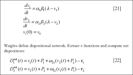
FIGURE 16. Two-Agent Coupled Model

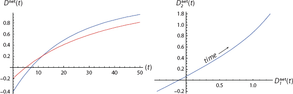
FIGURE 17. From Both Negative to Both Positive

Both net dispositions begin negative in the left graph and, so, in the −/− quadrant of the right graph. Then, on the left, while Blue is still negative, Red crosses his threshold at t = 5. This continues through the period 5 < t < 8, which is in the +/− quadrant on the right. Then, finally, at roughly t = 8, Blue goes positive and we arrive in the +/+ quadrant.

We embed this in a much richer story in Figure 18, which subsumes, in the simplest way, the core (e.g., lynching) example given in the Introduction. Richer renditions of that story will be presented in the three-agent mathematical versions to come and then spatiotemporally in the full agent-based model of Part II.

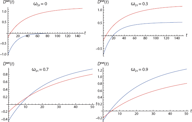
FIGURE 18. Dispositional Contagion

Simple Version of the Core Target

Referring to Figure 18 we see that, of his own volition, Agent 1 (Blue) would never act. This is shown in the upper-left frame, where ω₂₁ (the weight of 2 on 1) is zero. Agent 1’s initial affect and his immediate probability estimates are both zero. And, for these parameters, the Blue net disposition curve is never positive.⁹³

If we hike ω₂₁ to 0.3, Agent 1’s total disposition does exceed threshold (D ^net > 0), but he goes second and never exceeds Agent 2. The third frame (ω₂₁ = 0.7) was discussed earlier. Here, Agent 1 surpasses Agent 2 but still does not initiate the action. Finally, with ω₂₁ = 0.9 Agent 1 acts first and remains the most virulently committed throughout.⁹⁴

Now, in panel 4, where Agent 1 acts first, his observable behavior certainly suggests “leadership.” But, as we see, he is simply the most susceptible to dispositional contagion.⁹⁵ We will return to this distinction and the general discussion of leadership shortly.

Notice the role of the Rescorla-Wagner model in this two-agent story. If we cancel it (by setting Agent 1’s learning rate to zero) and also keep Agent 1’s probability (P) pegged at zero as before, then Agent 1’s net disposition reduces to

His highest disposition trajectory is obviously attained when ω₂₁ = 1. But, retaining our usual assumption of equal thresholds, this makes Agent 1 identical to Agent 2. This is still noteworthy in that alone, Agent 1 would sit at −τ₁, whereas with ω₂₁ = 1, he goose-steps across the threshold arm in arm with Agent 2. This is far from trivial. But with zero learning, he cannot go first—in the two-person case! As we shall see, in the three-person case, this is possible despite the fact that solo disposition net of threshold is negative. This is an important difference between the two-person and larger population cases.⁹⁶

The Full Trajectory

Returning now to the mathematical model development, all of this has had to do with the acquisition phase of Figure 15—the transition from −/− to the red zone of +/+. But the full trajectory returns to −/−. By what mechanism? Dispositional extinction, as illustrated in Figure 19, which picks up where Frame 4 of Figure 18 leaves off (t = 50). To be precise, this is the net disposition trajectory under affective extinction, as treated in the Rescorla-Wager model.⁹⁷ Of course, the agents are coupled through the weights. So, the extinction process, like the acquisition phase, would also exhibit contagion effects. But this example offers one realization of the troubling full trajectory of Figure 15. Notice that, as discussed earlier, the Blue agent’s dispositional extinction is steeper in Figure 19 than that of the Red agent. Both dispositions converge to asymptotic values because, as in equation [16], affects extinguish exponentially to zero, and all other net disposition terms are constants.

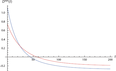
FIGURE 19. Dispositional Extinction to Benign State

Examples of Fear Contagion

Having shown that the basic model can generate them, is there actually evidence of interdependent affective trajectories, that a person can acquire fear through exposure to a conspecific’s expressions thereof, without direct experience of an aversive stimulus?

There is evidence of many sorts. Before reviewing it, we recall the earlier point that this capacity to acquire fear without direct conditioning is advantageous evolutionarily. “In particular, humans and other primates have developed social means of acquiring fears, which permit learning about the potential aversive properties of stimuli in the environment without necessarily having to experience the aversive event directly” (Ledoux and Phelps, 2008, p. 67).

Historical

Anecdotal evidence of emotional contagion is, of course, abundant. Gustave Le Bon (1895; 2001 ed.) wrote, “Sentiments, emotions, and ideas possess in crowds a contagious power as intense as that of microbes.”⁹⁸A panoply of contagious panics, phobias, and general hysterias is catalogued in Mackay’s compendious Extraordinary Popular Delusions and the Madness of Crowds (1841). Many of these—but most particularly the witch manias—are obviously fear based⁹⁹ and eventuated in gruesome violence. A prominent example is the Salem Witch mania, although the contagious fear and mutual suspicion of McCarthy’s witch hunts were no less virulent.

The fear-driven cat massacre of 1884 is a colorful example. This was stimulated by an outbreak of plague, presumed to be caused not by rats, but by cats. The ensuing cat massacre (in exterminating the rats’ main predator) only exacerbated the problem. This and many other historical examples are discussed in Hatfield, Cacioppo, and Rapson’s Emotional Contagion (1998).

A wealth of historical emotional contagion evidence from the field of public health is reviewed in J. M. Epstein et al. (2008), which develops mathematical and agent-based models coupling the contagion dynamics of fear and disease. Specifically, the model posits two epidemics: one of disease proper and one of fear of the disease. Fear stimulates changes in peoples’ contact behaviors (e.g., flight or self-isolation), and these behavioral adap-tations feed back to alter the disease trajectory. The coupled model offers a new, behavioral, mechanism to explain the multiple epidemic waves observed in the 1918 pandemic flu—a dynamic of long-standing interest to epidemiologists.

The R₀ of Fear

A fundamental parameter in epidemiology is the so-called basic reproductive rate of a disease. Termed the R₀—or R-naught—it is defined as the number of secondary infections resulting when a single infectious individual is placed in a population of susceptible individuals. In J. M. Epstein et al. (2008) we also develop a theoretical expression for the R₀ of fear and give the conditions under which it exceeds the R₀ of the underlying disease. Indeed, unlike prevalence–dependent models (Kremer, 1996; Philipson, 2000), fear can spread in the absence of disease.

An arresting contemporary health example of this is the case of Surat, India. “In 1994, hundreds of thousands of people fled the Indian city of Surat to escape pneumonic plague, although by World Health Organization criteria no cases were confirmed” (see J. M. Epstein, 2009). Fear-based refusal of effective vaccines is a related problem of widespread concern; it is central to the resurgence of polio, for example. In addition to violence and public health, the cascading financial crisis of 2008–2009 was clearly accelerated by a contagion of fear concerning the solvency of major financial institutions. Earlier examples of financial panics are discussed in Charles Kindleberger’s classic Manias, Panics, and Crashes (1978). Even olfactory stimuli are found: a sudden-onset epidemic of hysteria among schoolchildren, stimulated by an odor (!) is presented in G. W. Small et al. (1994). For further fascinating examples of what he terms the “social transmission of psychopathology,” see William Eaton’s The Sociology of Mental Disorders (2001). Recent research indicates that chemo-signals can also communicate human emotions, including fear and disgust (de Groot et al., 2012).

Adam Smith certainly believed in emotional contagion. In The Theory of Moral Sentiments (1759; 1982 ed.), he wrote, “the passions, upon some occasions, may seem to be transfused from one man to another, instantaneously and antecedent to any knowledge of what excited them in the first place.”

But, beyond historical analyses and innumerable anecdotes, there is also rigorous neuroscience to identify the underlying mechanisms.

Mechanisms of Fear Contagion

Jamesian Mechanisms—Facial and Postural Mimicry

Much of this work stems from the amazingly prescient theory of William James (1884), which centered on the view that unconscious mimicry of facial expressions stimulates emotional convergence: we first unconsciously mimic the other’s facial expression; our facial expression then triggers our emotion.¹⁰⁰ On the latter point, the classic experiment is Strack, Martin, and Stepper (1988; see also Adelmann and Zajonc, 1989). A nice discussion is given by Kahneman (2011). The encoding of facial expressions into emotions is apparently innate and is observed even in humans blind from birth and thus unable to acquire this mapping by observation (Haviland-Jones and Wilson, 2008, p. 238). Indirect suggestive evidence to this effect is that motor disorders, such as Parkinson’s and Huntington’s disease, are associated with emotional deficits, perhaps because the actual emotional stimulus, one’s adoption of a facial expression, is blocked (de Gelder et al., 2004). The substantial literature on fear contagion through facial expression has been extended by de Gelder et al. to full body postures, “similar to what has so far been argued for automatic recognition of fear in facial expressions” (p. 16703). In fact, in very interesting recent experiments, Aviezer, Trope, and Todorov (2012) found that body cues can dominate facial expressions in our discrimination of others’ emotions. For a compact history of James’s ideas and their successors, see LeDoux (2009). A central work in this tradition is Hatfield, Cacioppo, and Rapson (1994).

Laboratory Neuroscience

Current neuroimaging studies shed further light on the acquisition of emotions such as fear through observation. Olsson, Nearing, and Phelps (2007, p. 1) report that “classical fear conditioning requires first-hand experience with an aversive event, which may not be how most fears are acquired in humans.” They write that “fear acquired indirectly through social observation, with no personal experience of the aversive event, engages similar neural mechanisms as fear conditioning.” Their study suggests that “indirectly attained fears may be as powerful as fears originating from direct experiences.” As earlier noted, the capacity to acquire fear by observation is highly adaptive, of course. Fear acquisition through “social observation and verbal communication” are “more efficient and associated with fewer risks than learning through direct aversive experience.”

The amygdala is centrally implicated in both direct and observational fear acquisition (LeDoux, 1996). In monkeys, observational fear learning has been shown to be similar to direct fear conditioning. Olsson, Nearing, and Phelps (2007) report, “In particular, work on observational fear-learning in monkeys has shown that the relationships between the magnitude of a learning model’s expressed distress, the observer’s immediate response to the model’s distress and the resulting fear-learning in the observer are similar to those existing between an US, UR and a CR in classical fear conditioning paradigms (Cook and Mineka, 1990; Mineka and Cook, 1993).” They continue, “A recent study directly comparing human fear-learning through conditioning, social observation and verbal instruction supports the same conclusion (Olsson and Phelps, 2004).”

The following experiment is very impressive and is described in full detail in Olsson, Nearing, and Phelps (2007). Summarizing, a set of individuals were directly fear-conditioned by repeated pairings of a blue square (the CS) and an electric shock (the US). The CR was measured both by skin conductance response (CSR) and by functional magnetic resonance imaging (fMRI). This direct fear-conditioning exercise was filmed. Then, the true subjects were instructed to watch the movie. After having done so, they received the same CS (the blue square) and, remarkably, their CRs were comparable to those of the directly conditioned individuals.

“Subjects in our study showed a robust fear response following observation, corroborating previous reports of comparable behavioral (Mineka et al., 1984; Mineka and Cook, 1993) and psychophysiological (Olsson and Phelps, 2004) expressions of fear following observational learning and fear conditioning” (Olsson, Nearing, and Phelps, 2007, p. 8).

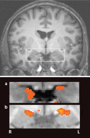
FIGURE 20. Observational Fear Conditioning. Source: Reprinted by permission from Macmillan Publishers Ltd: Nature Neuroscience (Olsson and Phelps 2007, p. 289), copyright 2007

Neuroanatomically, they add: “Importantly, our imaging data provides the first evidence that the amygdala, which is known to be critical to the acquisition and expression of conditioned fear (Phelps and LeDoux, 2005), is similarly recruited during the acquisition and expression of fear acquired indirectly through social observation” (Olsson, Nearing, and Phelps, 2007, p. 6).

Specifically, Panel a of Figure 20 shows the excitation pattern in the earlier Figure 5 for a subject after direct fear conditioning. Panel b shows the excitation pattern for a subject observing that same process of fear conditioning. Having watched that process, in other words, this is the observer’s response to the blue square (the CS). Again, detailed analysis of the comparison is given in LeDoux and Phelps (2008).

“Our finding that the formation and the expressions of fear through social observation relies on neural circuits that are similarly involved in fear conditioning is in accordance with the description of this form of learning as an evolutionarily old system for the transmission of emotionally relevant information, as documented in a wide range of species” (Olsson, Nearing, and Phelps, 2007, p. 10).

In sum, the Olsson, Nearing, and Phelps (2007, p. 10) results “show that fears learned by observing others engage the same neural mechanisms as fear acquired through direct experience, suggesting that social and nonsocial means of fear learning may be equally effective and powerful.”

So, yes, there is evidence that an individual’s fear may be “contracted” by another, without direct exposure to the aversive conditioning stimulus. Recent work on mirror neurons offers yet further reinforcement for emotional contagion, as do lesion studies (explored in Part II), “knock-out” animal models, and a wide variety of other approaches.

Mirror Neurons

Of such selective advantage is this capacity to acquire fear indirectly that we may even have evolved specialized neurons—so-called mirror neurons—for this purpose. Rizzolati and Fabbri-Desto contend that “ Mirror neurons are a distinct class of motor neurons that discharge both when individuals perform a specific motor act and when they observe the same act done by another individual” (Rizzolati and Fabbri-Desto, 2009, p. 337). See, for example, Rizzolatti and Craighero (2004), Iacoboni (2009), and Caramazza (2011).¹⁰¹

Experimental work by Gazzola, Van der Worp et al. (2007) suggests that actual imitative capacity is not necessary for the recruitment of relevant areas. Here, “Two aplasic individuals, born without arms or hands, were scanned while they observed hand actions. The results showed activations in the [usual] parieto-frontal circuit of the aplasic individuals while watching hand actions” (p. 344).

Contagion Beyond Immediate Vision

Emotional contagion can certainly occur outside of visual range. Obviously, blind people can acquire others’ fears through vocal cues, without literally seeing them. But emotional contagion can occur at any distance, by cell phone, field radio, text message, e-mail, tweet, and so forth.¹⁰² There is no question that, beyond cell phones, social media of all sorts played a major role in spreading the Arab Spring (discussed in Part III) and has been a central medium in the spread of widespread reactions to isolated events. For example, in 2012 a single independent YouTube video defamatory of Islam precipitated mass reactions across the Middle East, Southwest Asia, Indonesia, and Europe.¹⁰³ It is implausible that the majority of participants ever saw the video (were ever exposed to the primary stimulus), indicating that the disposition to protest was transmitted at long range by other means.

Heterogeneity

Finally, people exhibit heterogeneous susceptibility to emotional contagion. Hatfield, Cacioppo, and Rapson (1994) and Doherty (1998) develop an emotional contagion scale and demonstrate substantial variation across samples. The heterogeneous weights used in the mathematical and agent-based models here register this heterogeneity, which will be shown to play a central role in our understanding of so-called leadership and the evolution of collective behavior.

In sum, the phenomenon of emotional contagion is powerfully documented, and a diversity of neural mechanisms has been identified. Thus, while we are not modeling the brain proper, the brain science licenses the modeling. Affective contagion dynamics are crudely represented in the equations and are represented even more vividly in the agent-based model of Part II.

In the model, the probabilistic, nonemotional component of our behavior can also display strong contagion, or conformity, effects. Is this, too, supported by the neuroscience?

Conformist Empirical Estimates

The remarkable fact is that even a person’s empirical judgments are affected by those of other people. The most arresting example is the famous Asch (1956) experiment. Here, the mathematical judgment is much more primitive: Are two line segments of equal length? Asch’s hand-drawn original test figure is reproduced in Figure 21.

Obviously, in Asch’s experiment the lines did not carry labels betraying their true lengths (8 inches, and so on). Without them, the subject was shown the lines in Figure 21 and was asked to simply identify that line on the right that is the same length as the one on the left. When questioned alone (the control group), only 2 in 37 gave an incorrect answer. But in the presence of majorities unanimously giving erroneous answers,¹⁰⁴ the subjects’ judgments were strikingly different, as Asch (1956) reported:

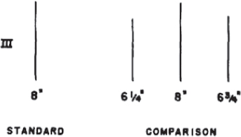
FIGURE 21. Critical Comparisons. Source: Asch (1956)

The estimates of the control group were virtually free of error. Thirty-five of 37 subjects made errorless estimates; of the remaining two subjects one showed one error, the other two errors. The proportion of errors was less than 1 per cent of the total number of critical estimates.

In contrast, the critical subjects showed a marked movement toward the majority. Errors increased strikingly, their frequency among individual subjects ranging from 0 to 12, or up to the maximum the conditions permitted. Only one-fourth of the subjects in the three experimental groups showed errorless performances, while in the control group 95 per cent were free of error. [Emphasis added.]

One might imagine that the subjects knew the right answers, and were just voicing the incorrect majority view to “go along.” This was certainly not the case uniformly. Having been told of their mistake in postexperimental interviews, many of the subjects concluded that their eyes or visual processing must have failed them, or that their head might have been tilted to produce an erroneous answer. But they did not deny that they believed what they had reported (Asch, 1956).

So, in fact, there are numerous sources of inaccuracy in the agent’s probability estimate: there is (a) sample selection bias, which may be damped or amplified by (b) memory, which may be damped or amplified by the (c) weighted estimates of others.

Asch, of course, did not have the benefit of contemporary neural imaging technology and hence was not able to suggest neurobiological correlates of conformity.¹⁰⁵ Recent studies—in addition to demonstrating arresting conformity effects—are beginning to do so.

Neural Basis for Conformity Effects

Berns et al. (2005) use a three-dimensional figure rather than Asch’s lines to clearly show conformity effects and the regions of interest in their connection.¹⁰⁶ In a fascinating section entitled, “The Pain of Independence,” (p. 252) the authors report, “The amygdala activation in our experiment was perhaps the clearest marker of the emotional load associated with standing up for one’s beliefs.”

The term pain is proving to be entirely justified. Recent work by Kross et al. (2011, p. 6270) shows that “ … when rejection is powerfully elicited … areas that support the sensory components of physical pain (secondary somatosensory cortex; dorsal posterior insula) become active.” The authors “… demonstrate the overlap between social rejection and physical pain in these areas by comparing both conditions in the same individuals using fMRI.” They find that “activation of these regions was highly diagnostic of physical pain, with positive predictive value of 88%.” As they write, “These results give new meaning to the idea that rejection ‘hurts’ … rejection and physical pain are similar not only in that they are distressing—they share a common somatosensory representation as well.”

Their “whole brain” and “region of interest (ROI)” analyses are shown in Figure 22. Particularly arresting in both cases is the overlap between social rejection and physical pain in S2 (the secondary somatosensory cortex).

This is highly original work. Kross et al. (2011, p. 6272) appropriately report that “… intense social rejection activated somatosensory regions that are strongly associated with physical pain, which are virtually never associated with emotion as typically studied.” Earlier, we discussed the evidence for observational fear conditioning (Olsson, Nearing, and Phelps, 2007). Kross et al. (p. 6274) raise the parallel question, “whether observing someone else experiencing intense social (rather than physical) pain (i.e., a parent witnessing their child’s rejection) also recruits sensory-pain processing regions.” This would help explain why public displays of social rejection—such as shunning—and, specifically, public punishment displays (e.g., the town-square pillory) are so effective in enforcing norms.

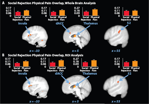
FIGURE 22. Social Rejection and Physical Pain. Neural overlap between social rejection and physical pain. (A) A whole-brain conjunction analysis revealed that regions typically involved in both the affective [AI (−30, 11, 14); dACC (9, 26, 24)] and sensory [thalamus (6, −4, 7); S2 (62, −28, 36)] components of physical pain were also involved in response to social rejection (ex-partner > friend) and physical pain (hot > warm). (B) An ROI analysis performed on physical pain regions revealed overlap between social rejection and physical pain in regions similar to those identified by the whole-brain analysis [AI (−33, 11, 14); dACC (6, 26, 24); thalamus (6, −4, 7); S2 (59, −26, 24)]. Bar graphs demonstrate the β-values for social rejection (ex-partner > friend) and physical pain (hot > warm) extracted from each cluster. Error bars represent one SE. None of the β-values associated with social rejection differed significantly from the β-values associated with physical pain (all two-tailed paired sample t statistics < 1.75, all P values > 0.09). Source: Kross et al. (2011, p. 6271); reprinted courtesy of PNAS

Evolutionarily, one might hypothesize that conformity is required for organized group defense. Groups incapable of powerful conformity are selected out in the intergroup competition. Hence, groups whose mem-bers are equipped with powerful wiring in this conformist direction—as where social rejection physically hurts—will enjoy selective advantage and are the ones that will be observed, as they are in Figure 22. A different, individual-level, evolutionary argument would be that social ostracism undermines mating opportunities. The species thus evolves mechanisms making it physically painful to engage in actions that threaten social acceptance and mating opportunities—literal self-punishment and deterrence are at work inside the individual.

As suggested earlier, however, the cost of this bias toward conformity is that it suppresses individual innovation and (painful) independence. Understanding this evolved source of our conformist impulses may equip us to overcome them, expressing the dissent so essential to democracy.

Thus, not only is there a vast psychology literature establishing conformity effects, but there is emerging a fascinating literature explaining them at a deeper neural level. Emboldened by all of this research, then, let us proceed to further elaborate the mathematical model assuming conformity effects, en route to the full spatial agent-based treatment of Part II. Many of the preceding topics will arise again in developing the agent-based model to follow. Hopefully, the foregoing historical, psychological, and neuroscience discussions are sufficient to justify the continuing model exposition.

Generalizing Rescorla-Wagner

This is a reasonable place to generalize the Rescorla-Wagner model slightly to accommodate a wider variety of learning trajectories. The generalized one-person model is shown in Figure 23.

The original model is the special case of δ = 0. The case, δ = 1 yields classic s-curve learning. Both these cases are analytically solvable. For δ strictly between 0 and 1, numerical methods are needed. I will use Mathematica’s nonlinear differential equation solver NDSolve, but a standard numerical approach like fourth-order Runge-Kutta will give indistinguishable results. All Mathematica Code is given in Appendix II and on the book’s Princeton University Press Website.

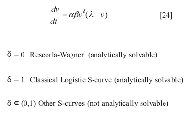
FIGURE 23. Generalizing Rescorla-Wagner

Nontrivial Majorities: The Three-Agent Model

We have discussed the two-agent model. But, for nontrivial forms of group decision, such as voting systems or juries, we require three or more individuals. This allows majority rule, which we model next. Extending the earlier two-person model directly, we introduce a third agent, as depicted in Figure 24. All agents are now equipped with the generalized model.

To see how this works, let us walk through the algorithm from the perspective of Agent 1, understanding that I am not claiming that any of this is knowingly executed by any human. The claim, as always, is that Agent_Zero is theoretically fruitful, not that it is descriptive.

With this in mind, let us colloquially say that person 1 first “solves” her generalized Rescorla-Wagner differential equation for v(t), where t indexes an exogenous stream of direct conditioning trials, which may be null. She then computes her probability estimate P₁ (in the subsequent spatial agent model, this will be the result of local sampling). If she placed no weight on the affect or probability estimates of others, she would simply subtract her threshold from this sum and act accordingly. But, in general, she “catches” the dispositions of others. The six weights indicated in the diagram register the fraction of the others’ (solo) dispositions contracted by each agent—through facial expressions, vocal cues, text messages, or other neurosocial mechanisms, as discussed earlier. This overall sum—the total disposition—is what each agent “compares” to his or her threshold.

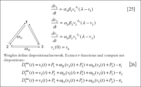
FIGURE 24. Generalized Three-Agent Model

The Central Case

I will now show two mathematical versions of our central case: the person who leads the lynch mob despite (a) harboring no aversion to black people (v is always zero), (b) having no evidence of black wrongdoing (P is always zero), (c) the same action threshold as everyone else, and (d) no orders.

Case 1: Homogeneous Classical Rescorla-Wagner Learners (All δ’s Zero)

First, I have made Agents 1 (Blue) and 2 (Red) literally identical to produce the simplest version. So their (rising) curves coincide (appearing as a single purple curve). If Agent 3 (Green) is completely invulnerable to dispositional contagion (ω₁₃ = ω₂₃ = 0), then his disposition simply sits at −τ, as shown in the left panel of Figure 25. He would never act. However, if he is maximally susceptible to dispositional contagion (ω₁₃ = ω₂₃ = 1), we generate the trajectory on the right, in which he goes first.

This is the simplest version of the central result. However, we have not exploited the generalized version of the model, which allows heterogeneity in learning modes (e.g., S-curve learning). This interesting heterogeneity comes from the δ’s.

Case 2: Heterogeneous Nonclassical Learners

Introducing δ > 0 enriches the learning trajectories substantially, as we shall see.¹⁰⁷ Again, we show two runs (Figure 26).

In the left panel, our protagonist (Green Agent 3), left to his own devices (i.e., with ω₁₃ = ω₂₃ = 0) would never act—net disposition is negative throughout, and his empirical probability estimate is zero throughout. However, with positive weight on the other agents’ (solo) dispositions, Agent 3 again initiates the lynch mob, as shown in the right panel. Agents 1 and 2 are S-curve learners, with δ’s of 1.0 and 0.5, respectively (see Appendix II code). This produces much more interweaving of trajectories, including a period between 100 and 150, in which Agent 3 relinquishes, but then regains, the lead. Again, the essential point is that Agent 3 begins with the strongest negative disposition, but, through dispositional contagion, acts first, and after some jockeying with Agent 1, remains the most militantly committed to the course … a course he would not have adopted in isolation.¹⁰⁸

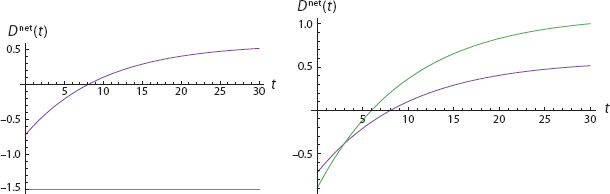
FIGURE 25. Homogeneous Classical Learners

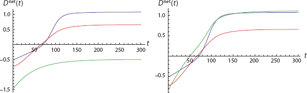
FIGURE 26. Heterogeneous Nonclassical Learners

Succession Does Not Imply Imitation

Once again, this is not an example of behavioral imitation. Agent 3 is first to behave, so—ipso facto—cannot possibly be imitating anyone’s behavior! But, in the model, neither is 1 or 2 imitating 3’s behavior. Even those who act later are not imitating behavior. They cannot be. In the model, behavior is Boolean (0 or 1), and this binary variable doesn’t appear as an independent variable in the model. Now, when Agent 3 exceeds threshold (crosses the horizontal axis), none of the others have done so, and their (binary) behavior is still 0. However, their affect—their solo disposition—was transmitted, and this sufficed to trip Agent 3’s behavior. This is a fundamentally different picture than models of contagious behavior. This emerges even more starkly in the spatial agent-based version that follows.

Contra Great Man Theory

Is Agent 3 the “leader” of the group’s ultimately unanimous lynch-mob behavior? By and large, we tend to assume that the first to act is the “leader,” that he is the most committed to the rightness of his course, and the most passionate toward it, and that these qualities are what make him a “man of action” who inspires others. Here is a direct counterexample, suggesting that those who act first and are normally seen as “leaders” may have no dis-tinguishing attribute save especial susceptibility to dispositional contagion. The others do follow him in time, but it is not because he has inspired them, but because they have inspired him! I certainly hope this is seen as a useful attack on the “great man” theory of history.

Tolstoy: The First Agent Modeler

Its most brilliant critic, and perhaps the first agent-based modeler, was Tolstoy. Tolstoy’s War and Peace (1869; 1998 ed.) is, of course, a literary-historical masterpiece. But, its attack on the “great man” theory also foreshadows agent-based modeling. Tolstoy’s perspective is entirely bottom-up and generative. It is a shame he did not live to see the advent of agent-based modeling, in which his view of history as an “emergent phenomenon”¹⁰⁹ is being realized computationally.

Tolstoy writes, “There are two sides in the life of every man, his individual life which is more free the more abstract its interests, and his elemental swarm-life¹¹⁰ in which he inevitably obeys laws laid down for him.” Tolstoy calls history “… the unconscious general, swarm-life of mankind,” and abjures the historian’s focus on “the great man” (p. 647). He writes, “The ancients have left us model heroic poems in which the heroes furnish the whole interest of the story, and we are still unable to accustom ourselves to the fact that for our epoch histories of that kind are meaningless. …”

In what I read as an incredibly prescient anticipation of agent-based generative modeling, Tolstoy continues, “To study the laws of history, we must completely change the subject of our observation, must leave aside kings, ministers, and generals, and study the common, infinitesimally small elements by which the masses are moved. No one can say in how far it is possible for man to advance in this way towards an understanding of the laws of history; but it is evident that only along that path does the possibility of discovering the laws of history lie; and that as yet not a millionth part as much mental effort has been applied in this direction by historians as has been devoted to describing the actions of various kings, commanders, and ministers, and propounding reflections of their own concerning these actions” (p. 881). “Only by taking an infinitesimally small unit for observation (the differential of history, that is, the individual tendencies of men) and attaining to the art of integrating them (that is, finding the sum of these infinitesimals) can we hope to arrive at the laws of history” (p. 880). But what is this but to “grow” history from the bottom up in an individual-based model? The agent-based model is the appropriate tool for studying the swarm-life of man.

While Agent 3 is the first to act in Figure 26, he is no more “a bold leader” than the fish at the head of the school. Neither is he following the direct orders of anyone else.

Swarmocracy

This is why conspiracy is less disturbing than decentralized swarm totalitarianism, and why conspiracy theory is correspondingly less profound than Tolstoy. Conspiracy theory attributes to the conspirators the theorist’s own analysis of the situation and posits that the conspirators are cynically benefitting from that situation, as fully aware of it as the theorist. Sometimes this is certainly true, as in countless cases of industrial and political corruption. But, in a way, this is the easy case: chop off the head, and the conspiracy is done. If you are being attacked by a bear, one well-placed bullet solves the problem. But, that is not the swarm-life … if the enemy is the swarm of bees, no bullet works. The swarm is resilient to local disruption and endogenously reassembles and perpetuates itself. Those individuals—differentials of history—who find themselves at the head are not cynics; they actually believe the (often pernicious) mythology they propagate. That they obviously benefit from it does not make them cynics either. Indeed, the mythology itself permits them to infer their righteousness from their station, regardless of how their station may have been attained.

Summing up to here: we have constructed the central case, in mathematical form—the parable in which Agent_Zero initiates action through disposition contagion. In the discussion thus far the action has been violent, but we later offer many interpretations in which it is not.

Complex Contagion of Disposition

As noted earlier, three agents are required to depict majorities. But three are also required to depict the important phenomenon of complex contagion. In the case of many diseases, such as influenza or smallpox, a single exposure is sufficient to produce transmission. However, the transmission of attitudes, norms, fears, and other social signals may require multiple exposures, confirming exposures, if you will. Centola and Macy (2007) introduce the term complex contagion for these and demonstrate that complex contagion dynamics on networks differ fundamentally from simple contagion dynamics, indeed that certain basic results (e.g., the power of small world network structures) are not robust to the requirement of multiple (as few as two) exposures. Because they sum the weighted dispositions of other agents, the individuals in the present model can exhibit complex contagions. For example, the previous Blue agent (right panel of Figure 26) requires the confirming disposition of the Red agent to pull her over her threshold. Influenced only by the Green agent, she would not trip. But, reinforced by the third, she does.

Interdependent Dispositional Trajectories in 3-Space

The vector of dispositions (D₁(t), D₂(t), D₃(t)) from Figure 24 traces out a curve in 3-space, as illustrated in Figure 27.

Just as the thresholds defined a rectangle in the two-agent case, so the three agents’ thresholds now define a cube, (a box parallelepiped) depicted in blue. There is unanimity to act when the group space curve is outside the threshold cube, as shown in Figure 28.

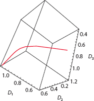
FIGURE 27. Group Dynamic as a Curve in 3-Space

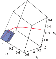
FIGURE 28. Unanimity When Group Trajectory Escapes Threshold Cube

A Mathematical Aside on Social Norms as Vector Fields

Obviously, these group trajectories (social movements, crowd behaviors) all take place in a social setting, which may be disapproving and resistant or supportive. These attitudes are local and can differ in different regions (neighborhoods of n-space in general). It is natural to think of these social norms as a resistant (or promotive) vector field through which the group trajectory is “working” to move.¹¹¹ How much social “work” is necessary to move from the origin to other positions in this milieu? That is the Line Integral of the trajectory in the Field, which we will compute and explore.

The examples thus far developed unfold in the degenerate “null vector field” of global indifference. The simplest significant departure from that would be the negative radial vector field directed toward the origin, itself representing the social state of absolute dispositional unanimity.

Negative Radial Moralities

The negative radial field assigns to each point in 3-space (R³) a vector directed toward the origin, with magnitude equal to the point’s distance from the origin. The farther from the origin the group members are, the stronger is the force directing them back to the origin. More relevantly, the more severely you violate a norm, the more severe is the pressure to return.

The radial vector field is F = (−x, −y, −z), where these entries are themselves real-valued scalar functions from R³ to R¹ (Marsden and Tromba, 2011; first edition 1976). This is shown in Figure 29.

As a purely heuristic start, some norms do work roughly this way. If you commit two murders, you get two life sentences. Fines for speeding increase with the level by which you exceed the speed limit. In orthodox Jewish law, the Mishna states the Law of Lashes for drinking, shaving, and becoming unclean (failing to wash after proximity to a corpse). Speaking of the Nazir¹¹² the Mishna reads, “If they said to him, “Do not drink, do not drink, and he drank, he is liable to lashes for each one”¹¹³ (Mishna Nezikin Makkot, Ch. 3).¹¹⁴ That is, the punishment, the restoring force, is additive with the number of transgressions … the number of steps from the norm. The same wording applies to the other violations: uncleanliness and shaving (Mishna Nezikin Makkot, Ch. 3). Adages such as “Let the punishment fit the crime” or “An eye for an eye; a tooth for a tooth” all express negative radial moralities, if you will.

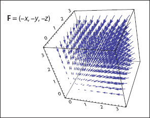
FIGURE 29. Negative Radial Vector Field

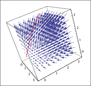
FIGURE 30. Group Trajectory in a Resistant Field

Now if we imagine the (red) group trajectory as it moves through the negative radial norm field, the picture is as in Figure 30.

To even the most lapsed of physicists, this picture veritably cries out for a line integral. Specifically, if we imagine the radial field as force, then we can compute the work (as in physics) required for the group to move out any given trajectory subject to the field (Figure 31).

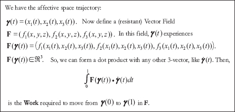
FIGURE 31. Social Work as a Line Integral

If F is centrist (negative radial), the group’s movement against it takes work, to a very surprising degree. If we just look at a straight-line trajectory directed away from the origin at 45 degrees to each axis, in a negative radial field (our earlier one multiplied by a scalar a, which was unity), and track the group’s total work in moving from the origin to any trajectory point (κ, κ, κ), the work is calculated as follows.

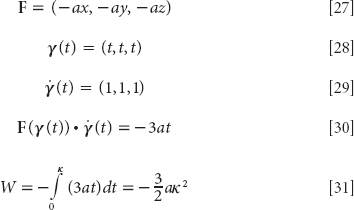
Very interestingly, the work is proportional to the square of κ. Hence, it is very hard to swim (far) against (even the unit negative radial) tide of convention. This applies only to the idealized negative radial field we’ve been exploring—a field that is irrotational (Curl F = 0) but compressible (Div F < 0). The true field, of course, is full of whirlpools, local equilibria, normative eddies, and moral turbulence. These would all be caused by inho-mogeneities in the field—such as neighborhood norms, social movements, and so forth—all worthy topics for further modeling.

Algorithm

To review this little mathematical excursion, the (original) Rescorla-Wagner initial-value problem is solvable analytically:

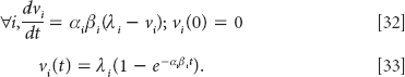
By substitution, so are the coupled net-of-threshold dispositions, .¹¹⁵

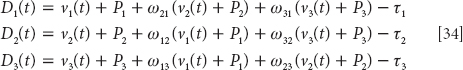
These are the components of the space-curve [35]:

Then we posited the centrist negative radial vector field (with the origin as its global attractor) F = a(−x, −y, −z). Denoting the space-curve’s derivative as , we form the dot product

Whence the work required is

The generalization to arbitrary n is direct. I have treated the resistant vector field of society as exogenous. Ultimately, of course, it is made up of all the other dispositions—all Tolstoy’s differentials of history—themselves the result of complex interactions.

Most discussions of learning cast trials as interactions between the experimenter and a subject. But, of course, interactions with other people are trials as well. There is no experimenter. In society, conditioning and extinction are underway concurrently, and in parallel.

This entire business of vector fields and their endogenization is a suitable topic for future research. Now, however, we return to the main plot of the book, without any embedding vector field—or, if you prefer, with only the null one.

Extinction of Majorities

Returning to the main plot, as discussed earlier, conditioning and extinction are not symmetrical. For example, recall that in Figure 26, agents crossed the threshold in the order Green, Red, Blue. But if we turn off all excitation trials at time 300, extinction (e.g., forgiveness, recalling our half-life discussion) occurs in a different order, namely, Red, Blue, Green, as shown in Figure 32. And the time to majority forgiveness is roughly half the time for majority excitation. Clearly, the space curve reenters the threshold cube (i.e., all curves in Figure 32 go negative) at approximately t = 35. Inside the cube, there is unanimous negative net disposition.

Posttraumatic Stress and Lambda

As mentioned earlier, the original Rescorla-Wagner model treats extinction by setting λ to zero when trials stop. But, as also noted, some people cannot set their λ to zero just because conditioning trials cease. They cannot free themselves of the negative association. This is often detrimental to the individual. But what is its effect on the group? With everything as in the previous simulation, if Agent 3 (Green) alone is traumatized and can cut her λ only to 0.95 rather than zero—as the other two can—everyone’s extinction trajectory is affected, as shown in Figure 33 (as compared to Figure 32). Now, Agent 3 is never able to extinguish the trauma. Moreover, the other agents take longer to do so, and they are not able to recover the same (negative) level of pretrauma dispositions as in Figure 32. So, the effects are dramatic and enduring. The hypothesis, in other words, would be that, in close-knit groups (i.e., where weights are high) subject to trauma, a single individual’s ongoing PTSD can delay and degrade everyone’s recovery. We will pick up this theme again in the agent-based model when we “lesion” one of the agents and study the effect on others in her network.

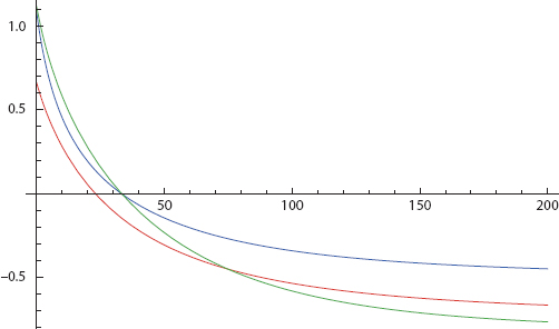
FIGURE 32. Majority Extinction

On historical scales, to extinguish collective distrust or enmity borne of sustained brutality and injustice (repeated aversive trials) may take more than their cessation, or even the good will of a new generation. Also, the negative association is easily reinstated by a recurrence of aversive experience (Rescorla and Heth, 1975; Norrholm et al., 2006; Bouton, 2004). In fact, the reinstatement can be more dramatic than on the initial trials. The wife cheats. The couple goes through extensive counseling. The husband’s trust is restored. If, after all that, the wife cheats again, it can be more surprising and salient than the first time. Likewise, revelations of racial health disparities today are amplified by the long shadow of Tuskegee.

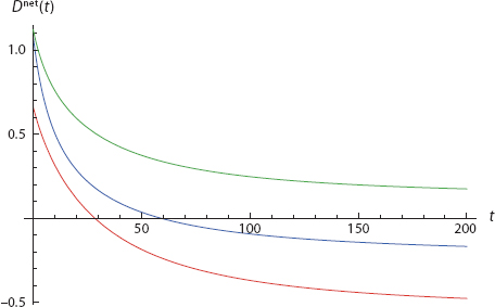
FIGURE 33. Extinction with One PTSD Individual

I.4. INTERIM CONCLUSIONS

The purely mathematical model, albeit highly abstract and very simple, does capture some core phenomena of interest. Behavior (the binary action adopted) is the result of affective, deliberative, and social modules. These are combined to form a total disposition (D^tot), which is compared to a threshold (τ). If D^tot exceeds τ,¹¹⁶ the agent acts; otherwise, she does not. Social networks are the medium over which social influence flows, but centrally, agents do not imitate one another’s binary behavior,¹¹⁷ but dispositions. Solo dispositions (each a sum of affect and probability judgments) are contagious via weights; if these conspire to produce total dispositions exceeding thresholds, observable behavior results. But the first agent to behave—the “leader”—may actually not be either the most passionate or the most convinced by evidence but, rather, may simply be the most susceptible to dispositional contagion, for which some current research support was offered. Asymmetries between fear acquisition and its extinction were noted, and the potentially large social effects of heterogeneous minimum λs (as a representation of PTSD) were briefly explored.

Mainly, we generated the central case: the agent who initiates the group’s behavior despite starting with the lowest disposition, with no initial emotional inclination (V = 0), no evidence (P = 0), the same threshold (τ) as all others, and no orders from above.

In fact, the preceding mathematical example begins with negative net disposition. The agent is actually disinclined toward the act of interest, be it violence, vaccine refusal, binge eating, or dumping toxic assets. But, through dispositional contagion, she is the first to act.

Revealing as it is, the simple coupled differential equation Agent_Zero model developed previously is quite unrealistic in three respects. First, the probabilities P are exogenous and fixed, rather than updating with recent direct experience or influence of others. Second, training trials are assumed to be arriving continuously, rather than in a discrete stochastic process. Third, the model is nonspatial. Agent-based modeling is a powerful way to include these features.

 

---

³⁹As discussed further in the context of lesion studies, the amygdala is not the only region recruited given fear-inducing stimuli. And the amygdala responds to stimuli that are not fear-inducing (Lindquist et al., 2011; LeDoux, 2012). But for the crude synthesis we have in mind, the following amygdalo centric exposition is pardonable.

⁴⁰Not “just any” pairings will work. The exact events that lead to neuronal change and association must be stipulated with great care. A seminal article correcting many widespread misunderstandings is Rescorla (1988).

⁴¹To be precise, it is stimulus-stimulus conditioning, as distinct from so-called operant conditioning or reinforcement learning.

⁴²To some readers, this language may suggest models in the general area of “cognitive architectures,” such as the SOAR model pioneered by Allen Newell. Here, I do not make use of models in this family. But see Laird, Newell, and Rosenbloom (1987).

⁴³In fact, an important step would be to increase model resolution, defining the agents to be neuronal complexes in their own right. Both the computational power and the underlying neuroscience are approaching the point where exploratory modeling “from synapses to societies” is feasible. This is discussed further under Future Research.

⁴⁴Relatedly, animals “play possum” to appear dead and, hence, unappealing as a meal.

⁴⁵This is an irresistible pun, because the word “amygdala” is Latin for almond.

⁴⁶“The lateral amygdala is generally viewed as the gatekeeper of the amygdala. It is the major site for receiving inputs from sensory systems—the visual, auditory, somatosensory (including pain), olfactory, and taste systems—to this region.” (LeDoux, 2007).

⁴⁷His analysis of why hair stands on end, through contraction of the occipitofrontalis, is among my favorites (Ch. XII). He also records that, in cases of extreme fear, “the intestines are affected. The sphincter muscles cease to act, and no longer retain the contents of the body.” The resulting name of this scared state does not require recitation here.

⁴⁸An important related article is Öhman and Soares (1994).

⁴⁹James (1884, p. 190) writes, “Our natural way of thinking about these standard emotions is that the mental perception of some fact excites the mental affection called the emotion and that this latter state of mind gives rise to the bodily expression. My thesis on the contrary is that the bodily changes follow directly the PERCEPTION of the exciting fact, and that our feeling of the same changes as they occur IS the emotion. Common sense says, we lose our fortune, are sorry and weep; we meet a bear, are frightened and run; we are insulted by a rival, are angry and strike. The hypothesis here to be defended says that this order of sequence is incorrect, that the one mental state is not immediately induced by the other, that the bodily manifestations must first be interposed between, and that the more rational statement is that we feel sorry because we cry, angry because we strike, afraid because we tremble, and not that we cry, strike, or tremble, because we are sorry, angry, or fearful, as the case may be. Without the bodily states following on the perception, the latter would be purely cognitive in form, pale, colourless, destitute of emotional warmth. We might then see the bear, and judge it best to run, receive the insult and deem it right to strike, but we could not actually feel afraid or angry.” [Capitalizations are in the original.]

⁵⁰See Janis and Feshbach (1953); Higbee (1969); Pratkanis and Aronson (2001).

⁵¹Ivan Pavlov (1927). Pages refer to the unabridged Dover edition (1960).

⁵²See Pavlov (1927, p. 52). The extent and variety of experiments, the rigor with which they are recorded, and the objectivity and intelligence with which they are interpreted are exceptional. He won the 1905 Nobel Prize for his researches.

⁵³Indicated by the implication symbol, →.

⁵⁴See his “Association of Ideas.” In fact, it is the cornerstone of his famous argument that there is no rational basis for belief in causation.

⁵⁵He notes that infants who experience the pain of putting their finger in a candle form an indelible association between flames and pain long before they can “reason,” in his view.

⁵⁶In other conditioning contexts, this may not be the relevant conditioning metric, as Rescorla (1988) very clearly argues.

⁵⁷This is discussed in more detail in Part III, in connection with lesion studies.

⁵⁸Here, the term module refers to a software model component, not a brain region. I do not enter into the debate regarding the brain’s modularity. To block any confusion, I typically use the term component when referring to model constituents. An obvious line of future research would be to swapin alternative learning models for the Rescorla-Wagner model, such as temporal difference [Sutton and Barto (1981, p. 334), Pearce and Hall (1980), or more recent neural network models (Freeman and Skapura, 1991)]. I am not wedded to Rescorla-Wagner; I modify it in a number of ways and welcome other explorations, as discussed in the Future Research section.

⁵⁹Typically, we will use the uppercase V when the context is time independent, and the lower-case v when the context is time dependent, as in difference or differential equations.

⁶⁰I say “infamous” because the experiment falls far short of contemporary scientific (indeed, ethical) standards. Amazingly, Watson filmed this experiment, which may be viewed at http://www.youtube.com/watch?v=Xt0ucxOrPQE. For a full account, see Watson and Rayner (2000; original appeared in 1920). Much more compelling research on conditioning has been conducted since Watson’s vivid experiment, the Olsson and Phelps (2007) fMRI experiment reviewed earlier being a good example. Others are reviewed later.

⁶¹In differential equation form, , so the second derivative is −αβ<0. Hence the v curve is concave down, and we see diminishing marginal associative strength.

⁶²Starting with the first inequality, we divide through by λ and subtract 1 from both sides. Multiplying both sides by –1 reverses the inequality yielding . Now logging both sides we obtain t ln Dividing through by the negative quantity ln again reverses the inequality to yield the advertised relation (negative because and ln(x) is negative on this set).

⁶³In my civil violence model (J.M. Epstein, 2002, 2006), there is a computational experiment comparing (a) a large (100%) absolute reduction in legitimacy that unfolds incrementally with (b) a much smaller (30%) absolute reduction, but in which the drop occurs in one step, not incrementally. The latter produces a much stronger public reaction in the model, consistent with Rescorla-Wagner.

⁶⁴This example comes from a talk John Cacioppo delivered at the Social and Behavioral Workshop, sponsored by the National Insitute for General Medical Sciences in Washington, DC, in November 2008.

⁶⁵This overarching point being true, the precise details of internment policy toward specific subpopulations (e.g., legal citizen vs. alien) of each group is quite tangled. See, for example: Semiannual Report of the War Relocation Authority for the period January 1 to June 30, 1946, not dated. Papers of Dillon S. Myer. Scanned image at trumanlibrary.org. Retrieved December, 2012.

⁶⁶For the full matrix version of the RW model, see Danks (2003).

⁶⁷I thank Robert Axelrod for this salient contrast. “All Japanese who lived on the West Coast of the United States were interned, while in Hawaii, where the 150,000-plus Japanese Americans composed over one-third of the population, an estimated 1,200 to 1,800 were interned,” http://en.wikipedia.org/wiki/Japanese_American_internment; Japanese Americans, from Relocation to Redress. 1991, page 135.

⁶⁸This was a common anti-Semitic myth in the interwar period in Austria and Germany.

⁶⁹Joseph McCarthy claimed to have revealed “a conspiracy on a scale so immense as to dwarf any previous such venture in the history of man.” Hofstadter (1964). As Hofstadter writes, “The paranoid spokesman sees the fate of conspiracy in apocalyptic terms—he traffics in the birth and death of whole worlds, whole political orders, whole systems of human values.” The images should be surprising and salient on a world scale.

⁷⁰Hebbian learning presumably evolved long before humans did.

⁷¹Even the experience of phantom limbs can eventually fade. Neurons with active function will literally displace those formerly engaged in the regulation of now-amputated limbs.

⁷²Figure 15 was drawn to reflect these properties.

⁷³Again, we specifically define: H(x − y) = 0 if x ≤ y and 1 if x > y.

⁷⁴The Mathematica movie code from which these screen shots were taken is Animate[Plot[Unit-Step[n − t](1 − Exp[−.15t]) + Unit-Step[t − n](1 − Exp[−.15n])Exp[−.15(t − n)], {t, 0, 65}, Plot-Range → {0, 1}], {n, 0, 30, .1}] also given in Appendix II.

⁷⁵Alternatively, the closer to horizontal is the acquisition curve, the closer to vertical is the extinction curve.

⁷⁶I am speaking somewhat figuratively here.

⁷⁷On the value of simple idealized models, see J. M. Epstein, (2008).

⁷⁸Similarly, so-called gravity models of economic interaction among cities posit that the force of attraction between agglomerations is proportional to the product of their sizes and is inversely proportional to a power of the distance between them, as in Newton’s law of universal gravitation. “Size,” of course, can be interpreted variously, and “distance” can be replaced with transportation cost, or effort required, none of which changes the gravity model parallel, for which I thank Robert Axelrod.

⁷⁹Once frightened by a snake, if you avoid all snakes, you never experience a harmless snake, and so you never lose your fear of all snakes. In the larger sociopolitical setting, the same inertia (never talking to members of a demonized out-group) can prolong intergroup hostility.

⁸⁰This admonition will certainly have a strange ring to it for those raised in the formal rational choice tradition, where it is affective dynamics that play virtually no role.

⁸¹Some would call this cognitive dissonance, á la Festinger (1957).

⁸²I thank Duncan Foley for suggesting this.

⁸³This P should not be confused with passion, although, admittedly, it would be a natural variable name.

⁸⁴Attentive readers will notice a tiny discrepancy with the action rule [3] of the Introduction. Using the earlier-developed terminology, solo disposition (V + P) would have to exceed twice the threshold, rather than simply the threshold. The reader may feel free to define the τ of Action Rule [3] as 2T, as defined here. But, in all candor, since we are not performing numerical calibration, I see no harm in ignoring it for notational convenience, and henceforth will.

⁸⁵The reader is invited to check that this obtains regardless of which variable, V or P, is playing the role of action proponent.

⁸⁶The spatial search radius is a user-adjustable slider (global variable) in the NetLogo Interface. NetLogo permits the user to toggle freely between Von Neumann and Moore neighborhoods. The latter includes the diagonal—NE, NW, SE, and SW—neighboring sites, for a total of eight for a radius of 1.

⁸⁷Base-rate neglect precludes proper Bayesian updating, because conditional probabilities are computed incorrectly. Bayes’ theorem is that: P(x|y) = P(y|x)[P(x)/P(y)]. The base rate refers to the bracketed term. Neglecting it leaves the so-called base rate fallacy that P(x|y) = P(y|x). This is quite a common, and very important, mistake. The probability of someone being a Muslim given that they are an Islamic terrorist, P(M|T), differs vastly from the probability that someone is a terrorist given simply that they are Muslim, P(T|M). Base-rate neglect equates the two, often producing baseless suspicion or worse. This is not to say that no people apply Bayes’ rule properly. But our agents use a different algorithm. An extension mentioned later is that agents could be Bayesians. The population might also be heterogeneous, with a mix of Bayesians and other inferential species.

⁸⁸The distinction between the mere existence of equilibria and their dynamic attainment in social systems is fundamental to the generative epistemology. For extended discussions see J. M. Epstein, 2006.

⁸⁹The term jihad admits a number of meanings, one of which is Holy War and another of which is internal struggle to obey the Koran.

⁹⁰Urchin sushi.

⁹¹Earlier model drafts tried putting the threshold term in the differential equations, for example. But if one simply adds τ to the right-hand side, the solution, v(t), becomes unbounded.

⁹²As powerful demonstrations of how difficult it is to characterize these rules formally, see S. D. Epstein (2000) and S. D. Epstein and Seely (2002).

⁹³This holds because the least upper bound is λ − τ and, since here they are both 1, the asymptotic value is zero. Note also that, if we fix both Agent 1’s affect (V) and probability (P) to zero, then his disposition trajectory is identical to Agent 2’s. So, while his initial affect is zero, we do give Agent 1 a small learning rate (αβ) so he has a distinguishable disposition trajectory. But this still does not exceed threshold. Of his own volition, he would never act. However, with dispositional contagion, he is the first to act, which is our target.

⁹⁴These cases unfold at quite different rates. Hence, for visual purposes, the t-axes differ among them.

⁹⁵This is to be distinguished from the case where the first to act simply has a lower threshold than everyone else. This may occur, but it is not the case here.

⁹⁶One could explore what Agent 1 learning trajectory, in a direction counter to Agent 2’s, is necessary to counter the latter’s influence, permitting 1 to stay negative.

⁹⁷The affective extinction component is handled in the Rescorla-Wagner model by setting λ to zero. This pulls down the disposition, as shown. But the disposition still includes the agents’ P-values and thresholds, τ. Thus, a subtlety of the extinction calculation is that the extinction rate applies to the purely affective components of the disposition, which in Figure 18, Frame 4, are roughly .86 and .60 when extinction begins. See Appendix II for full Mathematica programs.

⁹⁸Quoted in Hatfield, Cacioppo, and Rapson (1994, p. 105).

⁹⁹I say “obviously” because I presume there are, in fact, no witches. But that is probably a minority view.

¹⁰⁰In terms of the model, facial mimicry is not the imitation of a consequential binary behavior or action (e.g., join the lynch mob). It can contribute to the construction of one’s disposition. But it is the overall disposition’s relation to threshold that triggers action, as the latter is defined in this model.

¹⁰¹As a matter of sheer speculation, I wonder if mirror neurons explain why we laugh at pratfall humor. We know, through mirror neurons, how these incidents feel, and are laughing with relief as they befall someone else!

¹⁰²In monkeys, sounds expressing fear stimulate fright responses (freezing, flight). And in humans, communication (and dispositional contagion) can be vocal. On the vocal communication of emotion in humans, see Pittam and Scherer (1993, p. 340). We discussed the auditory route to the amygdala previously. Communications of emotion by text is another route, as reported in Funayama et al. (2001).

¹⁰³The bombing of the U.S. Embassy in Benghazi was distinct from these mass spontaneous demonstrations.

¹⁰⁴Asch varied the size of these confederate majorities but found that a majority of 3 was sufficient to produce a powerful “majority effect,” as he called this phenomenon.

¹⁰⁵On priming and conformity, see Epley and Gilovich (1999).

¹⁰⁶These are the amygdale [sic] and the right caudate nucleus. For quite different work on conformity, not involving geometric comparisons, see Spitzer et al. (2007, pp. 185–196).

¹⁰⁷However, this does impose a subtle constraint on the initial values of v. Unless one wishes to suppress all learning, these can be imperceptibly small—but cannot be literally zero. If δ > 0, then v₀ = 0 suppresses all learning. This is easiest to appreciate in the difference equation version. The first v-update would be there is no update because is 0. With which is 1. In the runs of Figure 26, I use 0.0001, which is effectively 0 in this context. For comparability, I use the same value in Figure 25.

¹⁰⁸The extinction curve is shown in Appendix II. The extinction order is different from the acquisition order.

¹⁰⁹I use the term emergent advisedly. For an energetic critique of classical emergentism, and its contemporary offspring, see J. M. Epstein (1998, 2006).

¹¹⁰I thank my fluent colleague and eminent Russia scholar Clifford Gaddy for wonderful discussions of Tolstoy’s usage here. He notes that Tolstoy’s precise term is ροевая, which is an adjectival form.

¹¹¹For rigorous definitions of norms and models of their dynamics, see Axelrod (1997a), Young (1993), and J. M. Epstein (2006).

¹¹²One who has foresworn alcohol, shaving, and sexual intercourse.

¹¹³In fact, the maximum is 39 lashes. I thank David Broniatowski and Julia Chelen for Talmudic researches.

¹¹⁴Chapters 1 and 3 of the fifth tractate Makkot of the fourth order Nezikin in the Mishna. Retrieved from http://halakhah.com/pdf/nezikin/Makkoth.pdf.

¹¹⁵We momentarily drop the superscript net to reduce visual clutter. Otherwise, these are identical to the formulae given in Figure 24.

¹¹⁶Equivalently, if D^net = D^tot − τ is positive.

¹¹⁷Technically, they do not register this.