II.1. Complete Solution of the Rescorla-Wagner Model in Step Functions
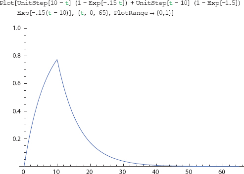
The following Mathematica 8.0 code implements equation [17], the complete acquisition and extinction trajectory for the Rescorla-Wagner model, using Heaviside unit step functions. The subsequent Animate code generates Animation 0 of this entire trajectory as the parameter, n, is varied from 0 to 30 in increments of 0.1. A snapshot (n = 10) from the movie is shown first. The full movie is posted as Animation 0 on the book’s Princeton University Press Website.
II.2. Two-Agent Dispositional Contagion: From Negative Disposition to Inititation of Action
The Four Panels of Figure 18 (includes Figure 17)
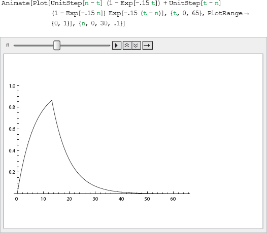
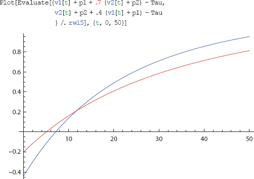
This entire section (and the next) can be compressed into a single Mathematica Module. But for nonprogrammers, a step-by-step exposition will be clearer. We begin by defining three global constants (probabilities and a common threshold) that will be used throughout. Note that Agent 1’s probability is zero. Then we use Mathematica’s nonlinear ordinary differential equation solver, NDSolve, to generate a numerical solution to the Rescorla-Wagner equations, with initial affect equal to zero for both agents. The S-curve exponent, delta, is also zero. Mathematica reports when it has computed Interpolating Functions, a message we shall suppress. Then we vary the weight of Agent 2 on Agent 1 from 0 to 0.9, showing the plots in each case. The pair of plots given in Figure 17 are from the 0.7 case shown next.

0 : Never positive

.3 : Positive but always lower

.7 : Supasses but goes second
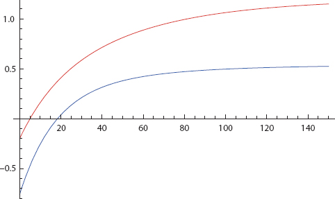
To plot the “phase portrait” of v1 on v2 with t as a parameter, we use ParametricPlot.

.9 : Goes first

To properly compute dispositional extinction trajectories from t = 50, one must first pull out the purely affective levels at that time and initialize the Rescorla-Wagner affective extinction variant at those values, which happen to be 0.86 and 0.60. Then NDSolve is used with λ = 0 to generate the purely affective extinction curves. Finally, we add the probabilities and subtract the thresholds to yield the full dispositional extinction trajectories given in Figure 19.

II.3. Three-Agent Runs: Homogeneous Classical Rescorla-Wagner Learners and Heterogeneous Nonclassical (Generalized) Rescorla-Wagner Learners
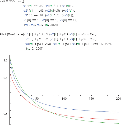
First, we generate the pair of runs in Figure 25. Agent 3 is the protagonist. In the first run, he assigns zero weight to the other two agents, who are identical (so their red and blue curves coincide, producing a purple curve). With no learning, Agent 3 sits at minus Tau. With maximal learning (weights of 1.0), he goes first. As discussed in the text, three agents is the minimum number required for this phenomenon.


Next, we exploit the heterogeneity afforded by the generalized model, generating the plots of Figure 26. Agent 3 remains a classical learner. But the others have diverse probability estimates and δ exponents, which make them S-curve learners. As usual, we first apply NDSolve to the generalized system of differential equations and then show two plots. With zero weights, Agent 3 never acts. With a weight of 0.475, he acts first and ends with the highest disposition.


Now, we generate the two extinction curves of Figures 32 and 33. In the first, no one has posttraumatic stress and all can reset their λ-values to zero. In the second, Agent 3 can reset only to 0.95, radically delaying her recovery (until t = 750), and substantially delaying everyone else’s. As before, we first solve the generalized Rescorla-Wagner equations for the purely affective trajectories, initializing at whatever value they attained when extinction begins. In this case, it is clear from the horiziontal net dispositions that the v-trajectories are close to their asymptotic values of 1.0, which we shall use. However, were that not the case, a cute way to extract approximate values, circumventing inspection of the interpolating functions, is to simply plot the affects from 299 to 300, for example, with the following command:
Plot[Evaluate[{v3[t], v2[t], v1[t]} /. rw6], {t, 299, 300}]
The extinction computations follow:

II.4. Group’s Disposition Trajectory in a Vector Field
These commands generate the vector field excursion reported in Part I. First, using VectorPlot3D, we generate the negative radial field of Figure 30 and store it as j1.

Then, we define the space curve with ParametricPlot3D and, in one move, invoke the Show command to superimpose them, as in Figure 31.

II.5. Strength-Homophily Dynamics
Here, we give Mathematica code for Figures 65, 66, and 67, where all agents are nonclassical with heterogeneous positive δ-values. First, we plot net dispositions and next we plot only the interagent weights over time. In both cases the weight is the sum of affective values times the quantity: 1 minus the absolute value of the affective difference. Third, the dynamic weight vector traces a curve in 3-space.


As a final example along these lines, we alter the learning rates of the agents to produce the hysteresis shown in Figure 68.
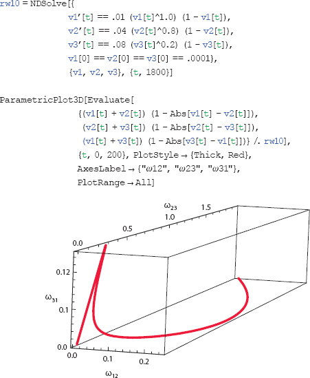
*As per footnote 107, δ > 0 requires positive initial affect. We use 0.0001 here and, purely for maximum comparability, in the preceding case.