

Mathematics is the art of effective reasoning. Progress in mathematics is encoded and communicated via its own language, a universal language that is understood and accepted throughout the world. Indeed, in appropriate contexts, communication via the language of mathematics is typically easier than communication via a natural language. This is because mathematical language is clear and concise.
Mathematical language is more than just the formulae that are instantly recognised as part of mathematics. The language is sometimes called mathematical “vernacular”1 because it is a form of natural language with its own style, idioms and conventions. It is impossible to teach mathematical vernacular, but we can summarise some of its vocabulary. This chapter is about elements of the vocabulary that occur in almost all mathematical texts, namely sets, predicates, functions and relations. Later chapters expand on these topics in further detail.
Mathematical notation is an integral part of the language of mathematics, so notational issues are a recurring theme in the chapter. Well-designed mathematical notation is of tremendous value in problem solving. By far the best example is the positional notation we use to denote numbers (for example, 12, 101, 1.31; note the use of “0” and the decimal point). Thanks to this notation, we are all able to perform numerical calculations that are unimaginable with Roman numerals. (Try multiplying MCIV by IV without translating to positional notation.)
Mathematical notation has evolved over centuries of use. Sometimes this has led to good notational conventions, but sometimes to poor conventions that are difficult to change. If you have experienced difficulty understanding mathematics, it may simply be that your difficulty is with a confusing notation.
In this text, we occasionally break with mathematical tradition and employ a nonstandard notation. Of course, such a step should never be taken lightly. Whenever we do, the reason is to improve understanding by improving uniformity.
12.1 VARIABLES, EXPRESSIONS AND LAWS
Mathematical expressions form an instantly recognisable part of mathematical language. Expressions like 2+3 and 4×5 are familiar to us all. These are examples of arithmetic expressions: their value is a number. Expressions often involve so-called constants: symbols that have a particular, unchanging value. The Greek symbol π, for example, is used in formulae for the perimeter and area of a circle. We say that it denotes a number (which happens to be approximately 3.1). “Denotes” means “is a notation for” or “stands for”.
Expressions are often confused with the values that they denote. Most of the time this causes no problems, but occasionally (as now) it is important to make a clear distinction. The analogy is with names of people: a name and the person it names are different things. For example, “Winston Churchill” is the name of a famous man; the name and the person are different. The name “Winston Churchill” has two parts, called the “forename” and “surname”, consisting respectively of seven and eight letters, while the person, Winston Churchill, has a date of birth, a mother and father, etc. However, when we refer to Winston Churchill, it is usually clear whether we mean the person or the name.
Expressions often involve variables. These are symbols that denote values that change (“vary”) depending on the context. In Einstein’s famous equation
E = mc2
c is a constant denoting the speed of light and E and m are both variables. The formula relates energy and mass; to evaluate energy using the formula we need to know the value of the mass m of the body in question. Similarly, the formulae 2πr and πr2 give the length of the perimeter and the area of a circle with radius r, respectively: π denotes a constant and r denotes a variable.
A class of expressions that is particularly important is the class of boolean expressions. These are the expressions that evaluate to one of the two boolean values, true or false. For example, 12=1, 0<1 and 1+2 = 2+1 are all examples of expressions that evaluate to true while 22=1, 1<0 and 1+1 = 1 are examples of expressions that evaluate to false. The value of expressions like m=0 and i<j, which depend on variables, can of course be either true or false; we cannot tell until we know the values of the variables.
(The name “boolean” is in recognition of George Boole (1815–1864) whose book The Laws of Thought introduced a calculus of reasoning, now called “boolean algebra”. Boolean algebra has evolved considerably since the publication of Boole’s book; we discuss it in Chapter 13. Boole’s book is available on the Internet through Project Gutenberg.)
Mathematics is traditionally about giving a catalogue of true statements. So traditional mathematics includes statements like “let m=0” and “suppose i<j” and the reader is meant to understand the boolean expressions as always evaluating to true. In computing, however, such expressions are used differently. For example, the expression “m=0” may be a test in a program; an action is chosen depending on the value of the expression, true or false, at the time that it is evaluated. In this text, our use of boolean expressions conforms to the computing scientist’s usage. This has important but sometimes subtle consequences.
One important consequence is how we deal with mathematical laws. An elementary example of a mathematical law is that adding 0 has no effect. Traditionally, the law would be expressed by the equation x+0 = x. Here x is a variable denoting a number and x+0 = x is a boolean expression; the law of arithmetic is that the expression evaluates to true whatever the value of x. There is thus an important difference between an expression like 0 = x and the expression x+0 = x, even though both are boolean expressions. The value of the former expression does depend on the value of x, while the value of the latter expression does not depend on the value of x. To emphasise the difference, we use square brackets to indicate that the value of a boolean expression is always true (i.e. the expression is a law), as in
[ x+0 = x ] .
The square brackets are pronounced “everywhere”. “Everywhere” is short for “for all values of the variables”. In the expression x+0 = x, the variable x is free; in the expression [ x+0 = x ] the variable x is bound. We discuss this terminology in more detail in Chapter 14.
Expressions have instances obtained by instantiating the variables in the expression. Instances of the expression x+0 are 0+0 and 1+0; these are instances where the variable x has been instantiated with numbers. Other instances are 2x + 0 and y2+0; here expressions are used to instantiate the variable x. Note that x is an expression as well as a variable, so 0, 1, 2x and y2 are all instances of the expression x.
If an expression includes more than one occurrence of a variable, it is important to instantiate every occurrence in the same way. For example, x2+x has instances 02+0 and 12+1, but x2+0 is not an instance of the expression.
Since laws are boolean expressions that are everywhere true, every instance of the expression also gives a law. The law [ x+0 = x ] has instances 0+0 = 0, 1+0 = 1, [ x×y + 0 = x×y ] and so on. Note that the everywhere brackets are not needed for statements like 1+0 = 1 because the expression does not include any variables.
12.2 SETS
The set is one of the most fundamental mathematical notions. It is best introduced by example: {Monday, Tuesday, Wednesday, Thursday, Friday} is the set of weekdays and {red, green, blue} is a set of primary colours.
In general, a set is defined by its elements. The set of weekdays has five elements: Monday, Tuesday, Wednesday, Thursday and Friday. The set of primary colours has three elements: red, green and blue.
These two examples both have a finite number of elements, and are sufficiently small that we are able to list all the elements. In the case of a (small) finite set, the set can be defined by enumerating (i.e. listing) its elements. The notation that is used is to enclose the list of elements in curly brackets. For example, {0,1} is a set with just two elements, while {a,b,c,d} is a set with four elements. The order in which the elements are listed is not significant. For example, the expressions {0,1} and {1,0} both denote the same set, the set with two elements 0 and 1.
The set {true,false}, whose elements are the two booleans, is particularly important. We use the abbreviation Bool for {true,false}.
12.2.1 The Membership Relation
The symbol “∈” is the standard notation for the so-called membership relation. The symbol is pronounced “is an element of” or “is a member of” or, most simply, just “in”. An expression of the form x∈S denotes a boolean value which is true if x is an element of the set S and false otherwise. For example, 0∈{0,1} is true while b∈{a,c,d} is false.
12.2.2 The Empty Set
An extreme example of a set with a finite number of elements is the empty set. The empty set has zero elements. It is usually denoted by the symbol “![]() ” but sometimes by {} (in line with the notation for other enumerated sets). It is an important example of a set, particularly in computing applications: the empty set is what is returned by an internet search engine when nothing matches with the given query. Formally, the empty set is such that x∈
” but sometimes by {} (in line with the notation for other enumerated sets). It is an important example of a set, particularly in computing applications: the empty set is what is returned by an internet search engine when nothing matches with the given query. Formally, the empty set is such that x∈![]() is
is false for all x.
12.2.3 Types/Universes
There is no restriction on the elements of a set. They can be colours, days, months, people, numbers, etc. They can also be sets. So, for example, {{0,1}} is a set with one element – the one element is the set {0,1}, which is a set with two elements. Another example of a set with one element is {![]() }; the single element of the set is the empty set,
}; the single element of the set is the empty set, ![]() . The two sets {
. The two sets {![]() } and
} and ![]() should not be confused; they are different because they have different elements.
should not be confused; they are different because they have different elements.
The word type is often used in a way that is almost synonymous with set. “Colour”, “day” and “number” are examples of “types”. Most often, the elements of a set all have the same type, but that is not a requirement. For example, {Monday,1} is a perfectly well-defined set; but it is not a set that is likely to occur in any meaningful application. In all the other examples of sets we have given so far, all the elements have had the same type. Mathematics texts often use the word universe instead of “type”; the elements of a set are drawn from a “universe” of values.
Basic types are the integers (numbers like 0, 10, −5), the natural numbers (integers at least zero; note that zero is included), the real numbers (which includes the integers but also includes numbers like ![]() and π), the booleans (
and π), the booleans (true and false) and characters (letters of some alphabet).
12.2.4 Union and Intersection
Two ways of combining sets are union and intersection. The union of two sets is the set formed by combining all the elements that are in (at least) one of the two sets. For example, the union of the sets {0,1} and {1,4} is {0,1,4}. We write
{0,1}⋃{1,4} = {0,1,4}.
The symbol “∪” denotes set union. Note that in this example two sets each with two elements combine to form a set with three elements (and not four).
The intersection of two sets is the set formed from the elements that are in both of the sets. The intersection of the sets {0,1} and {1,4} is {1}.We write
{0,1}∩{1,4} = {1}.
The symbol “∩” denotes set intersection.
Laws involving set union and set intersection are discussed in Chapter 13.
12.2.5 Set Comprehension
Defining a set by enumerating the elements becomes impractical very quickly, even for relatively small sets. The set of months in the year can, of course, be defined by enumeration but it is tedious to do so. The set of all days in a year can also be enumerated, but that would be very tedious indeed!
A very common way to define a set is called set comprehension. Set comprehension entails assuming that some set – the universe or type – is given, and then defining the set to be those elements of the universe that have a certain property.
For example, we may consider the set of all natural numbers that are at most one trillion and are divisible by 2 or 5. This is a finite set and so – in principle – it can be enumerated. However, enumerating its elements would take a long time, especially by a human being! In this example, the universe is the set of all natural numbers and the property is “at most one trillion and divisible by 2 or 5”. Another example is the set of all students at the University of Poppleton who are between the ages of 60 and 70. (This example may well be the empty set – the university may not exist and, if it does, there may be no students between the ages of 60 and 70.) The universe in this case is the set of students at the University of Poppleton, and the property is “between the ages of 60 and 70”.
The traditional mathematical notation for set comprehension is exemplified by
{n | 10 ≤ n ≤ 1000}.
This expression denotes the set of n such that n is in the range from 10 to 1000 (inclusive). The opening curly bracket is read as “the set of” and the “|” symbol is read as “such that”.
In this example – which is not atypical – it is not clear what the universe is. It could be the natural numbers or the real numbers. The variable n is a so-called dummy or bound variable. Texts often use a naming convention on variables because it avoids clutter. A common convention is that m and n stand for natural numbers, while x and y stand for real numbers. We often use this convention.
The expression
10 ≤ n ≤ 1000
is called a predicate on n. For some values of n, the expression is true (for example, 10, 11 and 12) and for some values it is false (for example, 0, 1 and 2). The expression {n | 10 ≤ n ≤ 1000} denotes the set of all (natural numbers) n for which the predicate 10 ≤ n ≤ 1000 evaluates to true.
The difference between free and bound variables is important. Expressions have values which depend on the values of their free variables, but it is meaningless to say that the value of an expression depends on the values of its bound variables. Because the expression {n | 10 ≤ n ≤ 1000} has no free variables, it denotes a constant. Compare this with
{n | 0 ≤ n < k}
which is an expression with one free variable, k. This is an expression denoting a set whose value depends on the value of the variable k. (By convention, k denotes a natural number.) One instance is {n | 0 ≤ n < 1}, which evaluates to {0} since 0 is the only instance of natural number n for which 0 ≤ n < 1 evaluates to true. Another instance is {n | 0 ≤ n < 2}, which evaluates to {0,1}. In general, {n | 0 ≤ n < k} denotes the set containing the first k natural numbers. The extreme case is {n | 0 ≤ n < 0}: the expression 0 ≤ n < 0 always has the value false irrespective of the value of n and so the set, {n | 0 ≤ n < 0}, is the empty set, ![]() . See Chapter 14 for further discussion of free and bound variables.
. See Chapter 14 for further discussion of free and bound variables.
12.2.6 Bags
Recall that a set is defined by its elements. That is, two sets are equal if they have the same elements. A bag is like a set but with each element is associated a number, which can be thought of as the number of times the element occurs in the bag. Bags are sometimes called multisets in order to suggest a set in which each element occurs a given multiple of times. Bags, rather than sets, are sometimes useful.
Some authors introduce special-purpose brackets replacing the curly brackets for sets, to denote a bag. We use the well-known curly brackets but write each element in the form m![]() x where m is a number and x is the element. For example, {2
x where m is a number and x is the element. For example, {2![]() red , 1
red , 1![]() green} denotes a bag of colours: two red and one green.
green} denotes a bag of colours: two red and one green.
12.3 FUNCTIONS
A function assigns outputs to inputs. More precisely, a function assigns to each element of a set of so-called input values a single output value. Familiar examples of functions are mother, father, and date of birth. In these examples, the “input” is a person and the “output” is some characteristic of that person; in all cases, the output is uniquely defined by the input – we all have just one mother, one father and one date of birth. Other familiar examples of functions are age and weight; because our age and weight change over time, the “input” is a combination of a person and a time. (For example, the age of Winston Churchill on VE Day was 61.)
Nationality is an example of a characteristic of a person that is not a function because some people have more than one nationality. Spouse is also not a function because some people do not have a spouse and, in polygamous societies, some have more than one. Nationality and spouse are examples of relations, a topic we return to shortly.
An example of a function in mathematics is even, which assigns the value true to the numbers 0, 2, 4, 6, etc. and the value false to the numbers 1, 3, 5, 7, etc. In this case, the set of inputs is the set of natural numbers and the set of outputs is the set of booleans.
The word “map” is often used to describe the action of a function, as in “the function even maps the even numbers to true and the odd numbers to false”.
In mathematics, there are lots of well-known functions that map real numbers to real numbers. Negation is the function that maps, for example, 0.1 to −0.1and −2 to 2. The square function maps, for example, 1 to 1, 2 to 4, 10 to 100, and 0.1 to 0.01. Note that the square function maps both 1 and −1 to 1; a function maps each input value to a single output value, but several input values may be mapped to the same output value. Other well-known functions are the sine, cosine and tangent functions, which map angles to reals, and area and volume. Area maps a two-dimensional object to a real number; volume does the same to a three-dimensional object.
12.3.1 Function Application
Functions are everywhere; they come in all shapes and sizes and there is a myriad of notations used to denote them and their application. The following are all commonly used notations for the application of well-known arithmetic functions to an argument x; the form that the notation takes is different in each case:
![]()
The examples illustrate the fact that functions may be written as prefixes to their argument (as in sin x and −x), as postfixes (as in x2, in which case it is common to write the function name as a superscript) or as parentheses (as in ⌊x⌋ ).
Additional notations that are used, typically for a temporary purpose, are exemplified by ![]() and
and ![]() . Sometimes it is not at all clear whether or not a function is being defined. The use of an overbar (as in
. Sometimes it is not at all clear whether or not a function is being defined. The use of an overbar (as in ![]() ), underlining (as in
), underlining (as in ![]() ) and primes (as in x′) are examples. When, say, x′ is used it could simply be an identifier having the same status as x or y, or it could be that a function is being introduced denoted by a prime and written as a postfix to its argument (for example, f′ is a standard notation for the derivative of f). An overbar is sometimes used as a replacement for parentheses (as in
) and primes (as in x′) are examples. When, say, x′ is used it could simply be an identifier having the same status as x or y, or it could be that a function is being introduced denoted by a prime and written as a postfix to its argument (for example, f′ is a standard notation for the derivative of f). An overbar is sometimes used as a replacement for parentheses (as in ![]() ) in order to indicate the scope of the function rather than being the name of a function, and sometimes to denote complementation. In the first case it does not denote a function, in the second case it does.
) in order to indicate the scope of the function rather than being the name of a function, and sometimes to denote complementation. In the first case it does not denote a function, in the second case it does.
A case where a function is defined but the function is seldom made explicit is when subscripts are used. If a text introduces two variables x0, x1, say, then x is a function with domain the two-element set {0,1}. Application of the function to an argument is denoted by subscripting. Similarly, if a sequence is denoted by x0, x1, ..., then x is a function with domain the natural numbers.
When introducing functions, standard mathematical vernacular can be mistifying. One often reads statements like “the function f(x) = 2x”. This is mathematical shorthand for several things at once. It is important to understand that the function is not f(x) = 2x and nor is it f(x). These are expressions with one free variable, x. The function that is being introduced in this example is the function that multiplies a number by 2; the statement gives it the name “f”. Another name for the function is the “doubling function”. Simultaneously, the statement states that application of the function to an argument will be written by enclosing the argument in parentheses and preceding it by the name “f”, as indicated by the pronunciation of f(x) as “eff of eks”. The symbol x in the statement is a dummy. Its choice has a hidden significance. To a large extent it is insignificant since one could equally write “the function f(y) = 2y”. The hidden significance is that it indicates that the function maps real numbers to real numbers since standard mathematical convention dictates that x denotes a real number. By way of comparison, the statement “the function f(n) = 2n” would implicitly define a function on natural numbers since mathematical convention dictates that n denotes a natural number. Finally, the boolean expression f(x) = 2x is a so-called definitional equality: because its purpose is to define the name “f”, it evaluates to true whatever the value of x.
Mathematical vernacular was copied in early programming languages. For example, FORTRAN, a programming language first developed in the 1950s, had the convention that variables beginning with the letters I thru N denoted integer values. But, in the course of time, it was realised that mathematical traditions are untenable in software development. For instance, much mathematical notation (such as juxtaposition, fx, for function application) relies on the names of variables and functions being a single symbol, but in computer programs it is inevitable that multi-character names like “person” and “age” are used. Modern programming languages require the names of variables and functions to be declared, making their types explicit, and different notations are used for function application. Some languages use a space for function application, as in age person; this is really just juxtaposition but the space is necessary for parsing purposes. Other languages use an infix dot, as in person.age. In this text, we try to heed the lessons of the computer age. But the reader will also have to get used to traditional mathematical shorthands in order to benefit from the vast wealth of mathematical literature. We have therefore adopted a compromise, in particular with regard to notation for functions and their application. In those parts of the text where there are long-standing mathematical conventions we adopt those conventions, but elsewhere we use non-conventional notation.
The examples above are all of functions with just one argument. They are called unary functions and the symbols used to denote them (such as the square-root symbol or the symbol “−” for negation) are called unary operators. When functions with two or more arguments are added to the list, the diversity becomes even greater. The most common notation for binary functions (functions with two arguments) is infix notation, as in a+b, where the operator is written in between the two operands. Sometimes, however, the function is not denoted (or denoted “by juxtaposition” in the jargon of mathematics) as is the case for multiplication in 2y; alternatively, it may be denoted by subscripting or superscripting as in xy, or using a two-dimensional notation as in ![]() . Another example is
. Another example is logbx. The two arguments are the base b of the logarithm and the argument x. (This example illustrates a general phenomenon whereby arguments that are relevant but the author wants you to ignore are hidden away as subscripts. They function a bit like the small print in legal documents.) In more advanced areas of mathematics, notations like ![]() are used.
are used.
12.3.2 Binary Operators
A binary function is a function that has two arguments. A binary operator is, strictly speaking, the symbol used to denote a binary function. For example, the symbols “+” and “×” are binary operators, denoting respectively addition and multiplication. Often, however, no distinction is made between the symbol and the function it denotes. Usually, it is clear from the context which is meant. In this text, we use “binary operator” to mean a function of two arguments, and we use “operator symbol” when we want to refer to the symbol itself. As mentioned earlier, binary operators are often written in infix form (as in 2+3 and 2×3), but sometimes they are written as prefixes to their arguments (as in log210 and gcd(10,12)). (The use of a prefix notation for greatest common divisors2 is an example of a bad choice of notation, as we see later.) They are rarely written in postfix form.
The symbols “![]() ” and “
” and “![]() ” will be used as variables standing for binary operators (in just the same way as we use m and n as variables standing for numbers). We write
” will be used as variables standing for binary operators (in just the same way as we use m and n as variables standing for numbers). We write ![]() and
and ![]() in infix form, but you should remember that they may also stand for binary operators that are not normally written in infix form.
in infix form, but you should remember that they may also stand for binary operators that are not normally written in infix form.
The symbols f and g will be used as variables to stand for unary functions. Their application to an argument will be denoted in this chapter in the traditional way, as exemplified by “f(x)”.
12.3.3 Operator Precedence
In any expression involving more than one function application, there is a danger of ambiguity in the order in which the functions are evaluated. Take, for example, the expression 8÷4÷2. The expression contains two instances of the division operator “÷” so there is a question about the order in which the operators are evaluated. Do we first evaluate 8÷4 (giving 2) and then evaluate 2÷2 (giving the final answer 1), or should 4÷2 be evaluated first (giving 2) and then 8÷2 (giving the final answer 4)? The two different evaluation orders are made clear by introducing parentheses: (8÷4)÷2 versus 8÷(4÷2). Another example is 842. This is, in fact, the same example except that division has been replaced by exponentiation. A third example is −23. Here the two functions are negation and exponentiation; the question is whether negation is evaluated before exponentiation, as in (−2)3, or the other way around, as in −(23). Of course, in this example it makes no difference – the answer is −8 in both cases – but it does make a difference in the expression −22.
Mathematical expressions are often ambiguous in this way. As we discuss below, the ambiguity can be deliberate and is exploited in mathematical calculations. This is the case when the ambiguity has no effect on the value of the expression. Where an ambiguity does have an effect on the value, the ambiguity is resolved by specifying an evaluation order and/or an order of precedence on the functions involved. The rules are often referred to as mathematical conventions. Unfortunately, because mathematical notation has evolved over centuries, traditional conventions are often not stated, causing difficulty for students. (Mathematicians often blame students for the resulting mistakes but should actually blame themselves!)
An example of a “well-known” convention is that subtraction is evaluated from left to right. For example, the expression 1−2−3 evaluates to −4 (i.e. (1−2)−3) and not 2 (which is the value of 1−(2−3)). In contrast, exponentiation is conventionally evaluated from right to left: the value of 1023 is 100 000 000 (i.e. 108) and not 1 000 000 (i.e. 1003). An example of where the order is irrelevant, and the resulting ambiguity exploited, is addition: 1+2+3 has the value 6 irrespective of whether addition is evaluated from left to right or from right to left. (See Section 12.5.4 for further discussion.)
Operator precedence is often necessary when different operators are involved. The best-known example of operator precedence is multiplication versus addition – the standard rule is that multiplication has precedence over addition. Thus when evaluating, say, 1 + 2×3 the value of 2×3 is first computed and then 1 is added to the result. If a different order of evaluation is demanded, this is indicated by the use of parentheses, as in (1+2)×3.
Elementary textbooks often do not mention precedence rules. One reason is that arithmetic notation has evolved in a way that avoids the need to explicitly state the rules. Multiplication is commonly denoted by juxtaposition which has the effect that in an expression like 1 + 2x the human eye naturally groups the symbols 2 and x together. This is also aided by the spaces around the “+” symbol. Similarly, in an expression like 2×32 the human eye naturally sees “32” as a group, thus suggesting the rule that exponentiation has precedence over multiplication. Adding more space, as in 2 × 32, also helps.
Another reason why operator precedence is not mentioned is that, sometimes, expressions are only meaningful if evaluated in a certain order. This is true of expressions like m ≤ n×p that involve a combination of arithmetic operators (like addition and multiplication) and relations (here the at-most relation denoted by “≤”). It just does not make sense to read this expression as “(m≤n)×p” because it does not make sense to multiply a boolean and a number. A convention on precedences is unnecessary.
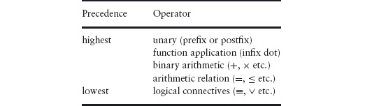
Identifying the structure of an expression is called parsing the expression. The parsing problem emerged as an important issue when programming languages were being developed in the 1960s. At that time, the problem was how to instruct a dumb machine to parse expressions of arbitrary complexity. But that experience made us aware that parsing is a problem for human beings too! The more complicated expressions become, the more difficult they become to parse, which is the first step towards understanding their meaning. Unfortunately, many mathematicians rely on the reader’s understanding of the meaning of an expression in order to understand its structure. This is a practice we eschew because clarity of expression is vital to problem solving. As a consequence, we strive to ensure that our expressions are easy to parse – wherever possible in the blink of an eye by the use of spacing and choice of operators. But precedence rules are unavoidable. The rules we use divide operators into a number of categories as shown in the table below. Within each category, further precedence rules apply, which are made clear when the operators are first introduced.
12.4 TYPES AND TYPE CHECKING
As mentioned in Section 12.2.3, the word “type” is often used synonymously with “set”. One difference is in the way that “types” are used to avoid mistakes, particularly in computer programs. The process is called “type checking”.
For many schoolchildren, the first encounter with type checking is in physics where “types” are called “dimensions”. The quantities that are measured (velocity, energy, power, etc.) all have a dimension; for example, the dimension of velocity is distance divided by time and the dimension of acceleration is distance divided by time squared. Whenever an equation is formulated in physics it is useful to check that both sides of the equation have the same dimension. It is relatively easy to do, and is useful in avoiding silly mistakes like equating a velocity with an acceleration.
Computer programs are unbelievably massive in comparison to the formulae used in physics and mathematics, and type checking plays a very significant role in the avoidance of error.
Type checking involves identifying certain base types and mechanisms for constructing more complex types from existing types. Examples of base types include the different types of numbers – natural numbers, integers and reals – and the booleans. These types are denoted by ![]() (the natural numbers),
(the natural numbers), ![]() (the integers),
(the integers), ![]() (the reals) and
(the reals) and Bool (the booleans). The simplest mechanisms for constructing more complex types are cartesian product, disjoint sum and function spaces. These three are discussed below. More complicated mechanisms include sets, matrices, polynomials and induction.
12.4.1 Cartesian Product and Disjoint Sum
If A and B are both sets, then their cartesian product, A×B, is the set of pairs (a, b), where a∈Aandb∈B. For example, taking A to be {red,green,blue} and B to be {true,false} then A×B is
{(red, true),(red, false) , (green, true) , (green, false),(blue, true),(blue, false)}.
The disjoint sum, A+B, of A and B is a set formed by choosing an element of A or an element of B and tagging the element to indicate from which of the two it was chosen. Various notations are used for the elements of A+B. Let us use l (for left) and r (for right) for the tags. Then the disjoint sum of {red,green,blue} and {true,false} is
{l.red , l.green , l.blue , r.true , r.false}.
Disjoint sum is sometimes called disjoint union because it has similarities to forming the union of two sets; indeed, in the example we have just given the disjoint sum of {red,green,blue} and {true,false} has exactly the same number of elements as the union of {red,green,blue} and {true,false}. Disjoint sum and set union differ when the two sets being combined have elements in common. In particular, for any set A, the set A+A has twice as many elements as the set A∪A. For example, {true,false}+{true,false} is
{l.true , l.false , r.true , r.false}.
The elements l.true and r.true are distinguished by their tags, as are l.false and r.false.
The use of the arithmetic operators × and + for cartesian product and disjoint sum is an example of overloading of notation. A symbol is “overloaded” if the symbol is used for different types of argument. (Readers familiar with modern programming languages will be aware of the problems of overloading. The symbol “/” is often overloaded so that 1/2 has a different meaning than 1.0/2.0, the former evaluating to 0 and the latter to 0.5. Type “coercions” are sometimes necessary in programs in order to enforce the desired meaning.) An explanation for the overloading is that it makes operations on sets look familiar even though they may be unfamiliar. This is deliberate and is based on correspondences between the two types of operator.
One correspondence is the number of elements in a set. If A and B are both finite sets with p and q elements, respectively, then A×B has p×q elements and A+B has p+q elements. Writing |C| for the number of elements in the (finite) set C, we have the laws
[ |A×B| = |A|×|B| ]
and
[ |A+B| = |A|+|B| ] .
(Recall the discussion of the square “everywhere” brackets in Section 12.1.) In both these equations, on the left “×” and “+” denote operations on sets, whereas on the right they denote operations on numbers. Recalling that ![]() denotes the empty set, we have
denotes the empty set, we have
|![]() | = 0.
| = 0.
As a consequence, for any finite set A,
|A+![]() | = |A|+|
| = |A|+|![]() | = |A|+0 = |A|.
| = |A|+0 = |A|.
Similarly,
[ |A×![]() | = |
| = |![]() | = 0 ] .
| = 0 ] .
Formally, the sets A+![]() and A are never the same, although they have the same number of elements – the difference is that all the elements of A+
and A are never the same, although they have the same number of elements – the difference is that all the elements of A+![]() have a tag. So we cannot write [A+
have a tag. So we cannot write [A+![]() = A]. When two (finite) sets have the same number of elements they are said to be isomorphic. The symbol “≅” is used to denote isomorphism, so we have the law
= A]. When two (finite) sets have the same number of elements they are said to be isomorphic. The symbol “≅” is used to denote isomorphism, so we have the law
[ A+![]() ≅ A ].
≅ A ].
Similarly,
[ A×![]() ≅
≅ ![]() ].
].
In the above paragraph, we limited the discussion to finite sets. However, the properties hold also for infinite sets. This involves some advanced mathematics which is beyond the scope of this text. The notion of “number” has to be extended to the so-called “transfinite” numbers and the number of elements of a set is called the cardinality of the set. That the properties hold for all sets, and not just finite sets, is a justification for overloading the notation.
12.4.2 Function Types
A function maps input values to output values. The type of a function therefore has two components, the type of the input and the type of the output. The type of the input values is called the domain and the type of the output values is called the range. We write
A→B
for the type of a function with domain A and range B. Examples are ![]() →
→Bool, the type of the function even which determines whether a given integer is even or odd, ![]() →
→![]() , the type of negation, doubling, squaring etc., and
, the type of negation, doubling, squaring etc., and ![]() →
→![]() , the type of the so-called floor and ceiling functions.
, the type of the so-called floor and ceiling functions.
The domain and range of a function are integral to its definition. For example, the process of adding 1 to a number has different properties depending on the type of the number. (See Section 15.1.) It is important, therefore, to distinguish between the function +1 of type ![]() →
→![]() and the function +1 of type
and the function +1 of type ![]() →
→![]() . The type of a function is particularly important when overloaded notation is used (for example, the use of + and × for operations on numbers and operations on sets).
. The type of a function is particularly important when overloaded notation is used (for example, the use of + and × for operations on numbers and operations on sets).
The domain type of a binary operator is a cartesian product of two types. Addition and multiplication of real numbers both have type ![]() ×
×![]() →
→ ![]() . Functions can also have functions as arguments; such functions are called higher-order functions. Function application is the first example we all encounter. As stated in Section 12.3.2, we use an infix dot to denote function application; every use of function application has type (A→B)×A → B for some types A and B. That is, the first argument of function application is a function of type A→B, for some A and B, and the second argument is a value of type A; the result of applying the function to the value then has type B. (Function application is an example of what computing scientists call a polymorphic function. There is not just one function application – there is a distinct instance for each pair of types A and B, but the distinction is not important. The simplest example of a polymorphic function is the so-called identity function. This is the function that maps every value to itself. There is an identity function for every type A.)
. Functions can also have functions as arguments; such functions are called higher-order functions. Function application is the first example we all encounter. As stated in Section 12.3.2, we use an infix dot to denote function application; every use of function application has type (A→B)×A → B for some types A and B. That is, the first argument of function application is a function of type A→B, for some A and B, and the second argument is a value of type A; the result of applying the function to the value then has type B. (Function application is an example of what computing scientists call a polymorphic function. There is not just one function application – there is a distinct instance for each pair of types A and B, but the distinction is not important. The simplest example of a polymorphic function is the so-called identity function. This is the function that maps every value to itself. There is an identity function for every type A.)
Function types are sometimes denoted by using superscripts. Instead of writing A→B the notation BA is used. This is done for the same reason that + and × are used for disjoint sum and cartesian product. It is the case that, for all sets A and B,
|BA| = |B||A|.
To see this for finite sets A and B, consider how one might define a function f of type A→B. For each element a of A there are |B| choices for the value of f(a). So, if A has one element there are |B| choices for f, if A has two elements, there are |B|×|B| choices for f, if A has three elements there are |B|×|B|×|B| choices for f, etc. That is, the number of different choices for f is |B||A|.
A consequence is that function spaces enjoy properties like exponentiation in normal arithmetic. For example,
![]() |AB+C| = |AB × AC|
|AB+C| = |AB × AC| ![]() .
.
Equivalently,
![]() AB+C ≅ AB × AC
AB+C ≅ AB × AC ![]() .
.
The sets AB+C and AB × AC are never the same (one is a set of functions, the other is a set of pairs) but they have the same cardinality. This is an important elementary property in combinatorics. See Section 16.8 for further discussion.
If arrow notation is used to denote function spaces, this rule (and others) looks less familiar and so may be less easy to remember:
[ (B+C) → A ≅ (B→A) × (C→A) ] .
The exponent notation is not used as frequently as the arrow notation but it is commonly used for the so-called power set of a set. A set A is a subset of a set B if every element of A is an element of the set B. The power set of set A is the set of all subsets of A. The subset relation is denoted by the symbol “![]() ”. For example, {Monday,Tuesday} is a subset of the set of weekdays, and the set of weekdays is a subset of the set of days. The empty set is a subset of every set and every set is a subset of itself so we have the two laws:
”. For example, {Monday,Tuesday} is a subset of the set of weekdays, and the set of weekdays is a subset of the set of days. The empty set is a subset of every set and every set is a subset of itself so we have the two laws:
![]()
The power set of the empty set has exactly one element (the empty set) and the power set of any non-empty set has at least two elements. One way of specifying a subset of a set A is to specify a function with range Bool and domain A; applied to an element of A, the function has value true if the element is in the subset and false otherwise. (This function is called the characteristic function of the subset.) The number of subsets of A is thus |BoolA|, which equals |Bool||A| (i.e. 2|A|). This suggests the notation 2A for the set of subsets of A – this is the explanation for the curious name “power set”. (Some authors use the notation ![]() (A), where the “
(A), where the “![]() ” abbreviates “power”, but then the motivation completely disappears.)
” abbreviates “power”, but then the motivation completely disappears.)
12.5 ALGEBRAIC PROPERTIES
The use of a mathematical notation aids problem solving because mathematical expressions are typically more concise than statements in natural language. Clarity is gained from economy of expression. But mathematical notation is not just an abbreviated form of natural language – the real benefit of mathematical expressions is in calculations.
All of the objects of mathematical discourse that we have introduced so far (numbers, sets, functions, etc.) have properties that are captured in mathematical laws. Such mathematical laws form the basis of mathematical calculations.
Arithmetic is the sort of calculations done with specific numbers, sometimes by hand and sometimes with the help of a calculator. An example of an arithmetic calculation is calculating income tax for an individual given their income and outgoings and the tax laws that are in force. Algebra is about calculations on arbitrary mathematical expressions and often involving objects and functions other than numbers and the standard arithmetic operators. Boolean algebra, for example, is about calculating with boolean expressions formed from the two boolean values true and false, variables (denoting boolean values) and the boolean operators, operators such as “conjunction” and “disjunction”. Relation algebra is about calculating with relations and operators such as “transitive closure”. We introduce these operators in later sections.
When studying new operators, mathematicians investigate whether or not certain kinds of algebraic law hold. Although much more general than arithmetic, the properties that one looks out for are very much informed by the laws of arithmetic. This section introduces the terminology that is used.
In the section, we use the symbols “![]() ” and “
” and “![]() ” as variables denoting binary operators. We assume that each operator has type A×A → A for some type A, called the carrier of the operator. Instances include addition, multiplication, minimum and maximum – for each of these the carrier is assumed to be
” as variables denoting binary operators. We assume that each operator has type A×A → A for some type A, called the carrier of the operator. Instances include addition, multiplication, minimum and maximum – for each of these the carrier is assumed to be ![]() (the set of real numbers). Other instances include set union, and intersection – for which the carrier is a power set 2A, for some A. We also use greatest common divisor (abbreviated
(the set of real numbers). Other instances include set union, and intersection – for which the carrier is a power set 2A, for some A. We also use greatest common divisor (abbreviated gcd) and least common multiple (abbreviated lcm) as examples. For these, the carrier is ![]() (the set of natural numbers).
(the set of natural numbers).
12.5.1 Symmetry
A binary operator ![]() is said to be symmetric (or commutative) if
is said to be symmetric (or commutative) if
[ x![]() y = y
y = y![]() x ] .
x ] .
(Recall that the square brackets are read as “everywhere” or, in this case, for all values of x and y in the carrier of the operator ![]() ;.)
;.)
Examples Addition and multiplication are symmetric binary operators:
The minimum and maximum operators on numbers are also symmetric. For the minimum of two numbers x and y, we write x↓y; for their maximum, we write x↑y. (We explain why we use an infix notation rather than the more common min(x, y) and max(x, y) shortly.)
Non-examples Division and exponentiation are not symmetric binary operators:
![]()
and
23 ≠ 32.
(To show that a property does not hold everywhere, we only need to give one counterexample.)
12.5.2 Zero and Unit
Suppose that ![]() is symmetric. Then the value z is said to be the zero of
is symmetric. Then the value z is said to be the zero of ![]() if,for all x,
if,for all x,
x![]() z = z.
z = z.
The value e is said to be the unit of ![]() if, for all x,
if, for all x,
x![]() e = x.
e = x.
The number 0 is the zero of multiplication, and the number 1 is the unit of multiplication. That is,
Note that 0 is the unit of addition since
Least common multiple (lcm) and greatest common divisor (gcd) are both symmetric operators. The number 0 is the zero of lcm,
and the number 1 is the unit of lcm,
Note that 0 is the only common multiple of m and 0 so it is inevitably the least.
For greatest common divisors, the terms “zero” and “unit” can, at first, be confusing. The zero of gcd is 1,
and the unit of gcd is 0,
(An instance of the unit rule is that 0 gcd 0 is 0. This may seem strange: how can 0 be a divisor of itself? The problem is that we have not yet given a precise definition of “greatest common divisor”. This we do in Section 12.7.)
There is no unit of minimum in ![]() . It is possible to augment
. It is possible to augment ![]() with a new number, called infinity and denoted by ∞. It then becomes necessary to extend the definition of addition, multiplication etc. to include this number. By definition, ∞ is the unit of minimum,
with a new number, called infinity and denoted by ∞. It then becomes necessary to extend the definition of addition, multiplication etc. to include this number. By definition, ∞ is the unit of minimum,
and the zero of maximum,
(The everywhere brackets now mean “for all x in ![]() ∪{∞}”.) Note that the introduction of infinity introduces complications when, as is usually the case, other operators such as addition and subtraction are involved.
∪{∞}”.) Note that the introduction of infinity introduces complications when, as is usually the case, other operators such as addition and subtraction are involved.
If the operator ![]() is not symmetric it is necessary to distinguish between a left zero and a right zero and between a left unit and a right unit. These definitions are easily given where necessary.
is not symmetric it is necessary to distinguish between a left zero and a right zero and between a left unit and a right unit. These definitions are easily given where necessary.
12.5.3 Idempotence
A binary operator ![]() is said to be idempotent if
is said to be idempotent if
[ x![]() x = x ] .
x = x ] .
Examples Minimum, maximum, greatest common divisor and least common multiple are all examples of idempotent operators. For example,
and
Set union and set intersection are also idempotent.
Non-examples Addition and multiplication are non-examples of idempotence since, for example, 1+1 ≠ 1 and 2×2 ≠ 2.
Typically (although not necessarily), idempotent operators are linked to “ordering relations”: minimum is linked to the at-least relation and greatest common divisor is linked to the divides relation. See Section 12.7.6 and the exercises at the end of the chapter.
12.5.4 Associativity
A binary operator ![]() is said to be associative if
is said to be associative if
[ x![]() (y
(y![]() z) = (x
z) = (x![]() y)
y)![]() z ] .
z ] .
Examples Addition and multiplication are associative binary operators:
Non-examples Division and exponentiation are not associative:
![]()
and
![]()
(In the second statement, we have used the symbol “^” for exponentiation, rather than the conventional superscript notation, because it makes the comparison with division clearer.)
When an operator is associative and it is denoted using an infix operator symbol we can omit parentheses, without fear of confusion, in a so-called continued expression. For example, the continued addition
1+2+3+4+5
is equal to (((1+2)+3)+4)+5, ((1+2)+3)+(4+5), (1+2)+(3+(4+5)) and so on. Parentheses indicate in what order the expression is to be evaluated but, because addition is associative, the order does not matter. This is a very, very important aspect of infix notation.
When an operator is symmetric as well as associative, we are free to rearrange terms in a continued expression as well as omit parentheses. For example,
2×4×5×25
is easiest to evaluate when written as
(2×5)×(4×25).
(This, of course, you would normally do in your head.)
We mentioned earlier that the usual prefix notation for greatest common divisors is a poor choice of notation. The reason is that “gcd” is associative and symmetric. That is, using prefix notation,
and
Try evaluating
gcd(5, gcd(10, gcd(24, 54))).
Now use an infix notation so that the problem becomes to evaluate
5 gcd 10 gcd 24 gcd 54.
The infix notation makes it much easier to spot that 5 gcd 24 equals 1, and so the value of the expression is 1. The prefix notation requires you to work out three different gcd values, beginning with 24 gcd 54, which is not so easy to do in your head.
Minimum and maximum are also commonly denoted by prefix operators but, because they are both associative and symmetric, it makes much more sense to write them as infix operators. Throughout this book, the symbol “↓” is used for minimum, and “↑” is used for maximum. For example,
u↓v↓w↓x
denotes the minimum of four values u, v, w and x.
12.5.5 Distributivity/Factorisation
A function f is said to distribute over the operator ![]() if there is an operator
if there is an operator ![]() such that
such that
![]() f(x
f(x![]() y) = f(x)
y) = f(x)![]() f(y)
f(y) ![]() .
.
Examples Multiplication distributes through addition:
Exponentiation also distributes through addition:
Note how addition changes to multiplication in the process of “distributing” the exponentiation over the terms in the addition. The function f in this example is “b to the power”. That is, it is the function that maps a value x to bx.
Because logarithms are the inverse of exponentiation, there is an inverse distributivity law:
Multiplication changes to addition in the process of “distributing” the logarithm over the terms in the multiplication.
(In each of these examples, we actually have a family of distributivity properties. For example, property (12.18) states that multiplication by x distributes through addition, for each value of x. So, multiplication by 2 (doubling) distributes through addition; so does multiplication by 3 and by 4, etc.)
Non-example Addition does not distribute through multiplication:
1+(2×3) ≠ ((1+2)×(1+3)).
Continued Expressions When a function distributes through an associative binary operator, the use of an infix notation is again very helpful. For example, 2× can be distributed through the addition in
2×(5+10+15+20)
to give
2×5 + 2×10 + 2×15 + 2×20.
The converse of distribution is called factorisation. The use of an infix notation is helpful in factorisation as well. For example, the log function can be factorised from
logb5 + logb10 + logb15 + logb20
giving
logb(5×10×15×20).
12.5.6 Algebras
The algebraic properties we have discussed are so important that mathematicians have studied them in great depth. The word “algebra” is used in, for example, “elementary algebra”, “boolean algebra” and “relation algebra” to mean the rules governing a collection of operators defined on a set (or collection of sets). (“Elementary algebra” is the collection of rules governing the arithmetic operators such as addition and multiplication on the real numbers.) Certain algebras are basic to many applications. In this section, we give the definitions of a “monoid”, a “group” and a “semiring”. Monoids and groups are quite universal. Semirings are basic to many path-finding problems. Elsewhere you will find definitions of “rings”, “fields” and “vector spaces”.
Definition 12.21 (Monoid) A monoid is a triple (A,1,×) where A is a set, 1 is an element of A and × is a binary operator on A. It is required that × is associative and 1 is the (left and right) unit of ×.
A monoid is said to be symmetric (or commutative) if × is symmetric.
The triple (![]() ,1,×) (the set of natural numbers, the number 1 and multiplication of numbers) is the archetypical example of a symmetric monoid. The triple (
,1,×) (the set of natural numbers, the number 1 and multiplication of numbers) is the archetypical example of a symmetric monoid. The triple (![]() ,0,+) is also a symmetric monoid.
,0,+) is also a symmetric monoid.
Definition 12.22 (Group) A group is a 4-tuple (A,1,×, −1) such that (A,1,×) is a monoid and −1 is a unary operator on A such that
![]() x×(x−1) = 1 = (x−1)×x
x×(x−1) = 1 = (x−1)×x ![]() .
.
A group is said to be abelian (or symmetric, or commutative) if the operator × is symmetric. (Other synonyms for abelian are symmetric and commutative.)
The 4-tuple (![]() ,0,+,−), where “−” denotes the unary negation operator and not binary subtraction, is an example of an abelian group. (The triple (
,0,+,−), where “−” denotes the unary negation operator and not binary subtraction, is an example of an abelian group. (The triple (![]() ,0,+) is a symmetric monoid and [ m + (−m) = 0 ].)
,0,+) is a symmetric monoid and [ m + (−m) = 0 ].)
Monoids and groups frequently arise when considering a set of transformations on an object (e.g. rotating and/or translating a physical three-dimensional object). The transformations form a group when each is “invertible” (i.e. the transformation can be reversed), otherwise they form a monoid. The unit is the do-nothing transformation. Section 11.2 gives an example of flipping the rows and columns of a 2 × 2 square.
Definition 12.23 (Semiring) A semiring is a 5-tuple (A,1,0,×,+) such that:
![]() (A,1,×) is a monoid;
(A,1,×) is a monoid;
![]() (A,0,+) is a symmetric monoid;
(A,0,+) is a symmetric monoid;
![]() × distributes over +,that is,
× distributes over +,that is,
[ x×(y+z) = (y×x)+(z×x) ]
and
[ (y+z)×x = (x×y)+(x×z) ] .
The operator × is said to be the product operator of the semiring and the operator + is said to be its addition operator. A semiring is idempotent if the operator + is idempotent.
Semirings are fundamental to the use of “quantifiers” (see Chapter 14) which are an integral part of many problems and, specifically, in path-finding problems. See Chapter 16 for a number of applications. A ring is a semiring (A,1,0,×,+) with an additional unary operator “−” (called the additive inverse operator) such that (A,0,+,−) is an abelian group.
12.6 BOOLEAN OPERATORS
Because set comprehension is such a ubiquitous method of defining sets, functions on booleans are very important. For example, corresponding to the union of sets, there is a binary operation from booleans to booleans called disjunction and, corresponding to intersection, there is a binary operation (also from booleans to booleans) called conjunction. Boolean-valued operators are relations; when the arguments are also booleans, the operators are called logical connectives because they relate (“connect”) the basic primitives of logic, the boolean values true and false. Equality is the most fundamental logical connective; implication is another. We introduce these boolean operators in this section. Chapter 13 goes into much more detail about their properties; see also Chapter 5.
Since the domain and range of boolean operators are (small) finite sets we can give them a precise mathematical meaning by simply enumerating all possible combinations of input and output value. This is done in a truth table.
There are two booleans and hence 22 functions that map a single boolean value into a boolean value. These four truth tables are as follows:

The first column of this table enumerates the different values that the variable p can take. Each of the columns after the vertical line lists the values returned by one of the four functions when applied to the input value p. In order from left to right, these are the constant-true function, the identity function, negation, and the constant-false function. The constant-true function always returns the value true and the constant-false function always returns the value false. The identity function returns the input value. Finally, negation returns false given input true and returns true given input false.
Because these are the only functions of type Bool→Bool any boolean expression in one boolean variable p can always be simplified to either true,p, ¬p, or false.
There are 22×2 (i.e. 16) binary functions from booleans to booleans. Eight correspond to the most frequently used ones: six binary operators and the constant true and false functions. These eight are shown in the following table:

To the left of the vertical line, all four different combinations of input values p and q are listed. To the right of the vertical line, the values returned by the eight binary operators are listed. Above each column is the notation that is used for the operator. From left to right, the operators are the constant-true function, (boolean) equality, (boolean) inequality, disjunction, conjunction, if, only if, and the constant-false function.
The truth table for equality needs no explanation: the value of p = q is true when p and q have the same value, and false otherwise. (For example, the value of true = true is true while the value of false = true is false.) Inequality (≠) is the opposite. Equality and inequality of booleans are also denoted by the symbols “≡” and “ ≢”, respectively. See Section 5.3 for further explanation.
Disjunction is also called “(logical) or” and conjunction is called “(logical) and”. The “or” of two booleans has the value true when at least one has the value true; the “and” of two booleans has the value true when both have the value true. The symbols “∨” and “∧” (pronounced “or” and “and”) are used to denote these operators. To enhance clarity, disjunction is sometimes called “inclusive-or” to distinguish it from “exclusive-or”; the “exclusive-or” of two booleans has the value true when exactly one of them has the value true. “Exclusive-or” is the same as “different from”, as can be checked by examining the truth table for inequality.
The symbol “⇐” is pronounced “if” or “follows from”. The value of false⇐true is false; all other values of p⇐q are true. The symbol “⇒” is pronounced “only if” or “implies”. The value of true⇒false is false; all other values of p⇒q are true.
12.7 BINARY RELATIONS
A binary relation is a function of two arguments that is boolean-valued. An example of a binary relation is the equality relation. Two objects of the same type (two numbers, two apples, two students, etc.) are either equal or not equal. Another example of a relation is the divides relation. Given two numbers, either the first divides the second or it does not.
Infix notation is often used for binary relations. This reflects the usual practice in natural language – we say “Anne is married to Bill” (the relation “is married to” is written between the two arguments), and “Anne is the sister of Clare”. (Note that “Anne is married to Bill” is either true or false.)
Relations are often depicted graphically. The values in the relation are the nodes in a graph and directed edges connect related values. As a simple example, consider the two letters “A” and “B” in the sequence “ABBA”. The letter “B” follows both the letter “A” and the letter “B”; the letter “A” follows only the letter “B”. We can depict the “follows” relation in a graph with two nodes, labelled “A” and “B”, and three edges. This is shown in Figure 12.1(a). Figure 12.1(b) shows the follows relation on the letters “C” and “D” in the sequence “CCDD”. Note the arrows – the arrow from D to C indicates that D follows C. It is not the case that C follows D.

![]() Figure 12.1: The follows relation on the letters in the sequences (a) ABBA and (b) CCDD.
Figure 12.1: The follows relation on the letters in the sequences (a) ABBA and (b) CCDD.
A genealogy tree depicts the “is a parent of” relation on members of a family. (A genealogy tree also depicts the ancestor relation – see the discussion of Hasse diagrams below.) Arrows are often not drawn on a genealogy tree because the dates shown make them unnecessary.
Important properties of binary relations are reflexivity, symmetry and transitivity. We discuss these in turn and explain how the use of an infix notation helps to exploit the properties.
Examples of relations that are used below include the at-most relation on numbers, denoted by “≤”, and the different-from relation on numbers, denoted by “≠”. A third example is the divides relation on integers, which we denote by the symbol “”. (So m is read as “m divides n”.) We say n is a multiple of m whenever there is some integer k such that m×k equals n and we say that m divides n whenever n is a multiple of m. For example, 3 divides 6 because 3×2 equals 6. It is important to note that every integer divides 0 because m×0 equals 0 for all m. That is,
[ m� ] .
In particular, 0�. In words, zero divides itself. If this seems odd, the problem is the use of the English word “divides” which may be understood differently. Here we have defined the divides relation to be the converse of the “is a multiple of” relation. This defines precisely the meaning of the word “divides” and it is important to stick to the definition. Do not confuse m
with ![]() or m÷n; the former is a boolean while the latter two are numbers.
or m÷n; the former is a boolean while the latter two are numbers.
The variables R, S and T will be used to stand for binary relations.
12.7.1 Reflexivity
A relation R is reflexive if
[ x R x ] .
Examples Equality is a reflexive relation:
The at-most relation on numbers is reflexive:
(Warning: learn to pronounce “≤” as “at most”. Saying “less than or equal to” is an awful mouthful! It also has the disadvantage that it suggests a case analysis on “less than” and “equal to” when reasoning about the operator; case analyses should be avoided wherever possible. Similarly, pronounce “≥” as “at least” rather than “greater than or equal to”.)
The divides relation is reflexive:
(Note the convention: m denotes an integer.)
An example of an everyday reflexive relation is “has the same birthday as” (everyone has the same birthday as themselves). Note that this is just equality (“the same”) in disguise; generally, if f is an arbitrary function, we get a reflexive relation by defining x and y to be related whenever f(x) equals f(y). In this example, the function is “birthday”. Indeed, the same trick is used to construct relations with properties other than reflexivity, in particular so-called “equivalence relations”. See Section 12.7.8 for details.
Non-examples The less-than relation on numbers is not reflexive:
0 < 0 ≡ false.
(This is sometimes written “0 ![]() 0”. By a common mathematical convention, “
0”. By a common mathematical convention, “![]() ” denotes the complement of the less-than relation; it so happens that
” denotes the complement of the less-than relation; it so happens that ![]() is reflexive, i.e. [ x
is reflexive, i.e. [ x ![]() x ].) The different-from relation is not reflexive. (No value is different from itself.) The “is a sibling of” relation on family members is also not reflexive. No one is a sibling of themselves.
x ].) The different-from relation is not reflexive. (No value is different from itself.) The “is a sibling of” relation on family members is also not reflexive. No one is a sibling of themselves.
12.7.2 Symmetry
A relation R is symmetric if
[ x R y = y R x ] .
Recall that a relation is a boolean-valued function. So x R y is either true or false, depending on the values of x and y. Similarly, the value of y R x is either true or false, depending on the values of x and y. A relation is symmetric if the value of x R y is equal to the value of y R x whatever the values of x and y.
Examples Equality is a symmetric relation:
The different-from relation is symmetric:
An example of an everyday symmetric relation is “is married to”.
These examples may seem confusing at first. Natural language is focused on true statements, and it is unnatural to allow false statements. George Boole, who originated the “boolean values”, had the great insight that a statement can have the value true or false. This means that we can compare them for equality. For given values of x and y, the expression x = y evaluates to either true or false (for example, 0 = 0 has the value true, and 0 = 1 has the value false). The symmetry of equality states that the value of x = y is always the same as the value of y = x.
(To appreciate the confusion of natural language better, note that the symmetry of equality means that x = 0 is the same as 0 = x. However, many people are very reluctant to write “0 = x” because it seems to be a statement about 0, in contrast to the statement “x = 0”, which seems to be a statement about x. You will need to unlearn this “natural” or “intuitive” way of thinking; train yourself to accept George Boole’s insight that they are identical.)
Non-examples The at-most relation on numbers is not symmetric:
(0 ≤ 1) ≠ (1 ≤ 0).
The value of 0 ≤ 1 is true, and the value of 1 ≤ 0 is false, and true and false are not equal. The divides relation is not symmetric:
12 ≠ 21.
12.7.3 Converse
The converse of relation R is the relation R∪ defined by
For example, the converse of “at most” (≤) is “at least” (≥) and the converse of the divides relation is the “is a multiple of” relation. Note that a relation R is symmetric exactly when R and R∪ are equal. We do not use the notation R∪, but we often refer to the converse of a (non-symmetric) relation.
12.7.4 Transitivity
A relation R is said to be transitive if, for all x, y and z, whenever x R y is true and y R z is true, it is also the case that x R z is true.
Examples Equality is a transitive relation:
(Recall that the symbol “⋀” means “and” and the symbol “⇒” means “implies” or “only if”.)
The at-most relation on numbers is transitive:
The divides relation is transitive:
(Read this as: for all m, n and p, if m divides n and n divides p then m divides p.)
Non-examples The different-from relation is not transitive. We have 0 ≠ 1 and 1 ≠ 0 but this does not imply that 0 ≠ 0. Formally, 0 ≠1 ⋀ 1 ≠0 ≤ 0≠0 has the value false.
The “child of” relation is clearly not transitive. Perhaps surprisingly, the sibling relation is also not transitive. Because it is symmetric, if it were transitive it would also be reflexive, which we know is not the case. For example, suppose Ann is a sibling of Bob. Then Bob is a sibling of Ann. Now suppose the sibling relation is transitive. Then it follows that Ann is a sibling of Ann. But no one is a sibling of themself. So the sibling relation cannot be transitive.
Note how unreliable the use of natural language can be. “Siblings of siblings are siblings” sounds perfectly plausible, but it is false.
Continued Expressions When a relation is transitive, it is often used in continued expressions. We might write, for example, m ≤ n ≤ p. Here, the expression must be read conjunctionally:the meaningism ≤ n and n ≤ p. In this way, the formula is more compact (since n is not written twice). Moreover, we are guided to the inference that m ≤ p. The transitivity of the at-most relation is implicit in the notation.
Similarly, we might write m = n = p. This too should be read conjunctionally. And, because equality is transitive, we infer directly that m = p. This is what is happening in a calculation like the one below. (In the calculation A, B and C are sets. Refer back to Section 12.4 for discussion of the laws that are used in the calculation.)
|AB+C|
= { law: [ |AB| = |A||B| ]with B:= B+C }
|A||B+C|
= { law: [ |A+B| = |A|+|B| ] with A,B := B,C }
|A||B|+|C|
= { exponentiation distributes over addition }
|A||B| × |A||C|
= { law: [ |AB| = |A||B| ] used twice,
the second time with B := C }
|AB| × |AC|
= { law: [ |A × B| = |A| × |B| ] with A,B := AB,AC }
|AB × AC|.
The calculation asserts that each expression is equal to the following expression. But, just as importantly, it asserts that the first and the last expressions are equal. That is, the conclusion of the calculation is the law
![]() |AB+C| = |AB×AC|
|AB+C| = |AB×AC| ![]() .
.
(The everywhere brackets are introduced in the conclusion because at no point does the calculation depend on the values of A, B or C.) The advantage of the conjunctional meaning of a continued equality is that long expressions do not have to be written twice (which would make it harder to read and give greater scope for error) and the transitivity of equality comes for free.
Sometimes different relations are combined in continued expressions. For example, we might write 0 ≤ m < n. This is read conjunctionally as 0 ≤ m and m < n, from which we infer that 0 < n. Here, the inference is more complex since there are two relations involved. But it is an inference that is so fundamental that the notation is designed to facilitate its recognition.
12.7.5 Anti-symmetry
An anti-symmetric relation is a relation R such that, for all x and y, whenever x R y is true and y R x is true, it is the case that x and y are equal.
Examples The at-most relation on numbers is anti-symmetric:
The divides relation on natural numbers is anti-symmetric:
Non-examples The different-from relation is not anti-symmetric: 0 ≠ 1 and 1 ≠ 0, but it is not the case that 0 = 1.
The divides relation on integers is not anti-symmetric: 1 divides −1 and −1 divides 1, but 1 and −1 are not equal. This example shows that it is sometimes important to know the type of a relation; the type of a relation defines the set of values on which the relation is defined. The divides relation on natural numbers is not the same as the divides relation on integers; the two relations have different properties.
12.7.6 Orderings
A relation that is reflexive, transitive and anti-symmetric is called an ordering relation.
Examples The equality relation is an ordering relation.
The at-most relation is an ordering relation. It is an example of a so-called total ordering. That is, for all numbers x and y, either x ≤ y or y ≤ x.
The divides relation is an ordering relation. It is a partial ordering. This is because it is not the case that, for all natural numbers m and n, either m ornm. For example, it is neither the case that 2 divides 3 nor 3 divides 2.
We can now give a precise definition of the “greatest common divisor” of two numbers m and n. It is the greatest – in the partial ordering defined by the divides relation – number p such that pm and p
. Thus “greatest” does not mean with respect to the at-most relation on numbers. This explains why 0 gcd 0 equals 0. In the partial ordering defined by the divides relation, 0 is the greatest number because every number divides 0. There is, however, no “largest” divisor of 0, where “largest” means with respect to the at-most ordering on numbers. It would be very unfortunate indeed if 0 gcd 0 were not defined because then gcd would not be associative. (For example, (1 gcd 0) gcd 0 would equal 1 but 1 gcd (0 gcd 0) would be undefined.) See Section 15.3 for more details.
Hasse Diagrams Ordering relations are often depicted in a diagram, called a Hasse diagram. The values in the ordering are depicted by nodes in the diagram. Two values that are “ordered” are connected by an upward path, of edge-length zero or more, in the diagram. Figure 12.2 depicts a partial ordering of a set with six elements (named by the numbers from 0 thru 5).
The Hasse diagram does not actually depict the relation itself. Rather it depicts a relation whose so-called reflexive transitive closure is the relation of interest. For example, the Hasse diagram for the at-most relation on natural numbers (Figure 12.3(a)) actually depicts the predecessor relation (the relation that holds between a number m and m+1, but is true nowhere else). “At most” is the “reflexive transitive closure” of the predecessor relation. Similarly, Figure 12.3(b) is the Hasse diagram for the divides relation on the first six natural numbers but, even though 1 divides all numbers and 0 is divisible by all numbers, there is not an edge from the node labelled 1 to every node nor is there an edge to the node labelled 0 from every node. “Reflexive closure” means allowing paths of length zero – there is a path of length zero from each node to itself – and transitive closure means allowing paths of length two or more.
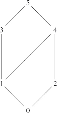
![]() Figure 12.2: Hasse diagram of a partial ordering.
Figure 12.2: Hasse diagram of a partial ordering.
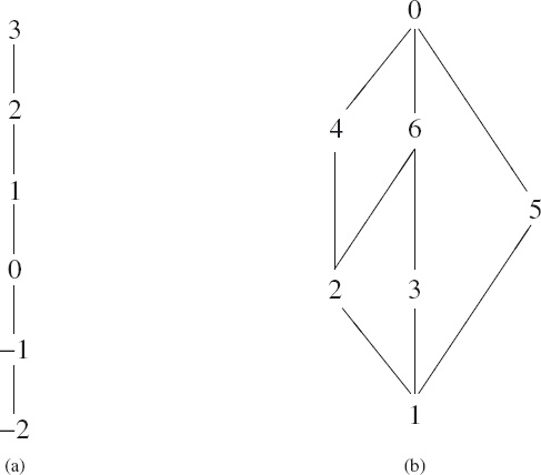
![]() Figure 12.3: (Partial) Hasse diagrams of (a) the at-most relation and (b) the divides relation.
Figure 12.3: (Partial) Hasse diagrams of (a) the at-most relation and (b) the divides relation.
Figure 12.4 shows (a) the reflexive closure, (b) the transitive closure and (c) the reflexive transitive closure of the relation shown earlier in Figure 12.2. The reflexive closure is simply formed by adding loops from each node to itself (thus making the relation reflexive). The transitive closure is formed by adding additional edges from one node to another where there is a path (upwards) of length two or more connecting the nodes (thus making the relation transitive). The convention that the relation holds between two numbers only if the level of the first is at most the level of the second applies to these figures.
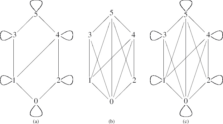
![]() Figure 12.4: (a) Reflexive closure, (b) transitive closure and (c) reflexive transitive closure.
Figure 12.4: (a) Reflexive closure, (b) transitive closure and (c) reflexive transitive closure.
A genealogy tree is a familiar example of “transitive closure”. Such a tree depicts the “is a parent of” relation, but, by following paths in the tree, we get the “is an ancestor of” relation. The ancestor relation is transitive, while the parent relation is not; the ancestor relation is the “transitive closure” of the parent relation.
Because there are no arrowheads on edges, a Hasse diagram is ambiguous about whether a relation or its converse is being depicted. A genealogy tree depicts the “is a parent of” relation but could also be construed as depicting the converse “is a child of” relation. We have described Figure 12.3 as depicting the at-most relation and the divides relation, but they can also be construed as depicting the at-least relation and the “is a multiple of” relation. Adding arrowheads always pointing up or always pointing down would remove the ambiguity, but the ambiguity is harmless because the converse of the reflexive transitive closure of a relation equals the reflexive transitive closure of the converse of the relation.
In conclusion, a Hasse diagram is an economical way of presenting a (small finite) ordering relation; it is easy for us to see paths through the graph and, in this way, the relation is made much clearer. It is an example of how economy of expression can be extremely helpful. When relations are too large to depict in a diagram, techniques for computing the transitive closure become very important; efficient algorithms for doing so are fundamental in computing science. See Section 16.2 for further discussion.
12.7.7 Equality
We have seen that equality is reflexive, symmetric and transitive. Equality is the most fundamental relation in mathematics, but it was a very long time before this was properly recognised. Indeed, the equality symbol was only introduced in 1557, which is very recent by mathematical standards, by Robert Recorde.3 Before then, when two expressions were equal they were written next to each other, leaving the reader to surmise their equality.
The importance of equality was properly recognised by Leibniz, who set himself the goal of reducing all mathematics to calculation (an extract from his writings is shown in Figure 12.5). Leibniz is acknowledged for formulating the first rule of logic – the rule of substitution of equals for equals. It is a rule that is used all the time in mathematical calculation, but lots of books fail to mention it. Here is a (very!) simple example of the use of Leibniz’s rule:
(2−1) × 3
= { arithmetic }
1 × 3.
The step uses the fact that 2−1 equals 1 in order to substitute the former by the latter.
Formulated precisely, Leibniz’s rule states that if f is a function and x and y are equal, then f(x) and f(y) are equal. In the above example, the function f is “multiply by 3” (×3).
Normally, when Leibniz’s rule is used, it is not necessary to be explicit about the function; “substitution of equals for equals” simply means that a subexpression of an expression can be replaced by an equal expression. In the example the subexpression “2−1” is replaced by “1”. Of course, it could also have been replaced by “3−2” or any other expression that equals 1.
Recorde’s symbol for equality is used universally to denote the fact that two values are the same. It is used, for example, for equality of numbers (integers, reals, complex numbers etc.), for equality of sets, for equality of functions, and so on. It is the most frequently encountered example of overloading of notation. On many occasions the overloading is beneficial, but sometimes it is not.
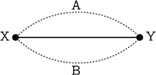
![]() Figure 12.5: Extract from Leibniz’s writings. [Lei69]
Figure 12.5: Extract from Leibniz’s writings. [Lei69]
12.7.8 Equivalence Relations
A common strategy in problem solving is to group together several objects that, for the purpose of solving the problem, are considered to be identical or “equivalent”. The underlying mathematical notion is an “equivalence relation”. An equivalence relation is a (binary) relation that is reflexive, symmetric and transitive. Equality is the simplest example of an equivalence relation.
Typically, an equivalence relation on a set A is defined by combining a function with domain A with the equality on the range of the function. For example, suppose we consider the function even of type ![]() →
→Bool. We define the relation “has the same parity as” on ![]() by, for all integers m and n,
by, for all integers m and n,
m has the same parity as n ≡ even(m) = even(n).
This relation groups all the even integers together and all the odd integers together. It is easily checked that the relation is reflexive: for all integers m,
m has the same parity as m
(because equality is reflexive). It is also symmetric: for all integers m and n,
m has the same parity as n ≡ n has the same parity as m
(because equality is symmetric). Finally, it is transitive: for all integers m, n and p,
m has the same parity as n ⋀ n has the same parity as p
⇒ m has the same parity as p
(because equality is transitive). That the relation is an equivalence relation is a direct consequence of the fact that equality is an equivalence relation and (implicitly) Leibniz’s rule of substitution of equals for equals.
In general, if A and B are sets and f is a function with domain A and range B, we can define a relation “has the same f value as” by determining, for all x and y in the domain A, the truth value of
f(x) = f(y).
(Note that “=” denotes equality in the range B.) We might, for example, regard two objects as equivalent if they have the same colour (red, blue, green etc.) or two people equivalent if they are the same age. Lots of other examples can be given. In this way, the function f is used to partition the set A into groups of “equivalent” elements.
An equivalence relation is, in fact, always defined in this way, at least in principle. Another way of defining an equivalence relation is to consider the reflexive, symmetric and transitive closure of a given relation. Each group of “equivalent” elements is called an equivalence class; treating each equivalence class as an object creates what is called a quotient space. This is an important mathematical construction, comparable in importance to disjoint sum and cartesian product.
12.8 CALCULATIONS
In this book, we use a style of presenting mathematical calculations that emphasises the documentation of the calculation. The style is quite self-explanatory and has already been used in Section 12.7.4. Here we spend a few words on explaining the style.
Let us base our explanation on a concrete example. Consider the following problem. A student buys a drink for themself and a friend. The friend’s drink costs 3 times as much as the student’s drink. The student pays with a 5-pound note and gets 1 pound in change. What is the cost of the drinks?
To solve the problem, we introduce two variables s and f for the cost of the student’s drink and the cost of the friend’s drink. We are given that f = 3×s and s+f+1 = 5. Now we can calculate:
f = 3×s ⋀ s+f+1 = 5
= { substitution of equals for equals }
f = 3×s ⋀ s + 3×s + 1 = 5
= { arithmetic }
f = 3×s ⋀ s = 1
= { substitution of equals for equals }
f = 3×1 ⋀ s = 1
= { arithmetic }
f = 3 ⋀ s = 1.
This calculation is deliberately simple so that we can focus on its structure rather than on the details of the specific problem.
The first thing to observe about the calculation is that its conclusion is an equality “everywhere” between the boolean expressions
f = 3×s ⋀ s+f+1 = 5
and
f = 3 ⋀ s = 1.
By “everywhere” we mean that the two expressions always have the same (boolean) value whatever the values of the variables f and s. For example, if f and s are both 0, the two expressions are both false; if f is 3 and s is 1, the two expressions are both true.
The calculation does not assert that f = 3 has the value true (or that s = 1 has the value true). It asserts no more and no less than that what is given has the same boolean value as the expression f = 3 ⋀ s = 1. This is an important aspect of boolean algebra. The logical connectives, like equality and conjunction, glue together primitive boolean expressions but they do not assert the truth or falsity of these expressions. In this example, the student and the friend may be arguing over the cost of the drinks; the calculation helps to simplify the argument but does no more.
The second thing to observe is that each line of the calculation is connected by boolean equality in just the same way as the calculation in Section 12.7.4 used set equality. The symbol “⇔” is sometimes used to denote boolean equality and, unfortunately, some readers may have been taught to read the symbol as “if and only if”. Even worse, some readers may have been taught to connect the statements by implication (⇒). The use of “if and only if” in this context is an over-complication. It is like calling equality of numbers “at most and at least” or equality of sets “is a subset of and is a superset of”. The use of implication is wrong in the same way that a calculation that concludes that 2×3 is at most 6 is wrong. The only argument for using a different symbol here for boolean equality is the overloading of the equality symbol in the same calculation: the equality symbol in “f = 3” is equality of numbers. However, the layout of the calculation eliminates any possible confusion.
The third thing to note about the calculation is that every step is accompanied by a hint. The challenges of programming have taught us that documentation is very important. Documentation of calculations is important as a check in the process of performing the calculation and as a reminder for later. The hints we use vary in detail. Sometimes they are very explicit and sometimes not. The hint “arithmetic”, for example, does not provide much information – we assume that the reader has no difficulty with arithmetic calculations – but it does indicate that the logical connectives in the formula (in this case ⋀) can be ignored and the reader’s attention should focus on the arithmetic operators. This can be very useful in more complicated calculations.
The hint “substitution of equals for equals” occurs twice in the above calculation. This refers to Leibniz’s first rule of logic which we introduced in Section 12.7.7. In fact, although the rule is only explicitly mentioned in two of the steps it is used in all four. In the second step the boolean s + 3×s + 1 = 5 is simplifed to s = 1 and this simplification is applied in the context of the function that maps p to f = 3×s ⋀ p. Similarly, in the final step 3×1 is substituted by its equal 3 in the context of the function that maps n to f = n ⋀ s = 1. Leibniz’s rule is fundamental to almost all calculations but often not mentioned explicitly. Its importance is another reason for our stressing boolean equality in preference to “if and only if”.
12.8.1 Steps in a Calculation
Our calculations have a number of steps (usually more than one). A two-step calculation might have the following shape.
R
= { p }
S
= { q }
T.
In this calculation, R, S and T are expressions, and p and q are hints why [ R = S ] and [ S = T ], respectively. The conclusion of the calculation is that [ R = T ]. (Recall that the square brackets means “everywhere”.)
The hints we use are often references to algebraic laws, either explicitly stated or just named. Here is an example of a step where the law is given explicitly:
(n+1)2 − n2
= { ![]() x2 − y2 = (x−y)×(x+y)
x2 − y2 = (x−y)×(x+y) ![]() ,
,
with x , y := n+1 , n }
((n+1) − n) × ((n+1) + n)
In this case, the step is an instance of a law of arithmetic. The law is enclosed in everywhere brackets to indicate that it is true for all (numbers) x and y and the details of the instance are indicated by the simultaneous assignment. We name the most commonly used laws (e.g. “associativity”) rather than state them explicitly. The very simplest rules (e.g. unit laws such as [ x+0 = x ]) are often applied silently.
Calculations quickly become very long if all steps are made explicit. To avoid this, we sometimes combine several steps into one. We might, for example, write
(n+1)2 − n2
= { arithmetic }
2×n + 1.
We only do so where the omitted calculation steps are expected to be familiar. This means that when we first introduce a topic we give each step in detail; as familiarity with the topic grows we permit ourselves to take larger steps. Mistakes most often occur in larger steps so our advice is be very cautious about combining many steps into one. A particular case is when applying a definition. Take care to state explicitly the substitutions that are being made for any parameters in the definition, and postpone any simplifications to subsequent steps.
12.8.2 Relations between Steps
A calculation with a number of steps, in which each step relates one expression to the next by equality, establishes that all the expressions are equal (everywhere). However, it is usually the equality between the first and last expressions that is important to us. Formally, we silently exploit the fact that equality is a transitive relation. That is, if R = S and S = T, it is also the case that R = T.
The less-than relation, denoted by “<”, is also transitive. Here is a calculation that constructs a rough estimate of the difference between 256 and 367.
< { 367 < 400 }
400 − 256
< { 200 < 256 }
400 − 200
= { arithmetic }
200.
The conclusion of this calculation is that 367 − 256 < 200. It illustrates the so-called conjunctional use of the less-than operator. In general, R < S < T means R < S and S < T. Transitivity of less-than means that a consequence of R < S < T is that R < T.
Different relations may be combined in the same proof, but then there should be a logical justification for doing so. For instance, one step of a proof may assert, say, R < S, whereas the next asserts S ≤ T. The inference is then that R < T. All such steps can be combined with equality steps, as in the last line above. However, it would be nonsense to combine < with > or ≥ in one calculation since then no inference can be made of the relation between the first and last expressions.
The type of the expressions is arbitrary. They may denote real values, integer values, sets, relations etc. In each case, the familiar equality symbol, “=”, is used to denote equality of values. In particular, if R, S and T denote boolean values we still use the equality symbol to denote equality. For example, a step in a proof might be
E ≤ F
= { E and F denote integer values.
Property of integer arithmetic }
E < F+1
Here we are using the fact that the boolean expression E ≤ F will always have the same value as the expression E < F+1 whenever E and F denote integer values. In other words, the value of E ≤ F (which is either true or false) is equal to the value of E < F+1. In in-line expressions, we often use the symbol “≡” to denote equality of boolean values. One reason for this is to avoid ambiguity. For example, we write
E ≤ F ≡ E < F+1
in order to avoid confusion with
E ≤ F = E < F+1
which means E ≤ F and F = E and E < F+1. (So equality here means equality of integer values rather than equality of boolean values.) There is another reason for having two notations for equality of boolean values, which is that boolean equality is both transitive and associative. This second reason, which is much more important than the first, is motivated in Section 5.3 and reviewed in Chapter 13.
It is important to realise that a boolean expression will typically evaluate to true or false depending on the values of its free variables. There are two ways in which we assert that a boolean expression always has the value true: the expression in a calculational step and when square brackets surround the expression. If the expression has no free variables the square brackets are omitted (as in 1−1 = 0).
Generally, in calculational steps, the connecting relations have lower precedence than the operators in the expressions they connect, this convention superseding any other precedence conventions. You should have no problem with this convention since it is clearly what is suggested by the layout.
12.8.3 “If” and “Only If”
Steps relating boolean values will sometimes be related by “if” or “only if”. The if relation is denoted by “⇐” and the only-if relation by “⇒”.
Here is an example of a calculation involving an if step. (Read the second step as 10×20 ≤ 11×23 if both 10×20 ≤ 11×20 and 11×20 ≤ 11×23.) It establishes that 200 ≤ 11×23 is true.
200 ≤ 11×23
= { 200 = 10×20 }
10×20 ≤ 11×23
⇐ { “≤” is a transitive relation }
10×20 ≤ 11×20 ≤ 11×23
= { multiplication is invertible with respect to “≤”
(applied twice), and 10 ≤ 11 and 20 ≤ 23 }
true.
An if step is a strengthening step. In this example, the inequality 10×20 ≤ 11×23 is replaced by the stronger statement 10×20 ≤ 11×20 ≤ 11×23. Because they are strengthening steps, if steps in calculations are much less welcome than equality steps; it may be the case that the strengthening is too coarse. In the following example, the pattern of the above calculation is used, but the strengthening leads to a property that cannot be established. As a consequence, the calculation stalls.
243 ≤ 11×23
= { 243 = 9×27 }
9×27 ≤ 11×23
⇐ { “≤” is a transitive relation }
9 × 27 ≤ 11 × 27 ≤ 11 × 23.
Note that the calculation is correct even though 11×27 ≤ 11×23 is false. The proposition “243 ≤ 11×23 if false” is a valid, although meaningless, conclusion.
Only-if steps are the converse of if steps; an only-if step is a weakening step. An important use of only-if steps is in determining circumstances in which a boolean expression is false. An example is the following:
23×11 = 243
⇒ { Leibniz (substitution of equals for equals) }
(23×11) mod 3 = 243 mod 3
= { (23×11) mod 3 = 1
243 mod 3 = 0
(details of calculation omitted) }
1 = 0
= { arithmetic }
false.
The first step should be read as “23×11 = 243 only if (23×11) mod 3 = 243 mod 3”. The step is unmistakably a direct application of Leibniz’s rule that when a function is applied to equal values it gives equal results. In this case, the function that is being applied is the “mod 3” function, which computes the remainder after dividing a given number by 3. The omitted details in the second step involve the use of properties of remainder computation which make it easy to evaluate (23×11) mod 3 (without evaluating 23×11) and 243 mod 3 (see Section 15.4). The conclusion is that 23×11 = 243 only if false,that is, 23×11 ≠ 243.
12.9 EXERCISES
1. Say which of the following are everywhere true. In the case where the expression is not everywhere true, give an instance where the expression is false. Assume that x ranges over the real numbers.
(a) 0 ≤ x2
(b) x < 2x
(c) x2−x−12 = (x≤3)×(x+4)
(d) x2+x−20 = (x−4)×(x+5)
(e) (−x)3 =−(x3)
2. Enumerate the elements of the following sets.
(a) {0,1,4}∪{4,1,3}
(b) {0,1,4}⋂{4,1,3}
(c) ({2,4,6}∪![]() ∪{9}) ⋂{9,4}
∪{9}) ⋂{9,4}
(d) {m | m ∈{0,1,4}∪{4,1,3} ⋀ even(m)}
(e) ![]() ⋂{2,4}
⋂{2,4}
(f) {0,1,4}+{4,1,3}
(g) {0,1}×{0,1}
(h) {0,1,2}+ ({1}×{3,5})
(i) 2{0}
3. Determine the number of elements in each of the following sets. Try to do so without enumerating all the elements.
(a) {m | 0 ≤ m < 1000}
(b) {m | 0 ≤ m < 1000}+{m | 2000 ≤ m < 2500}
(c) {0,1}×{m | 0 ≤ m < 1000}
(d) ![]()
(e) 2{m | 0 ≤ m < 3}
(f) {![]() , {a,b}}
, {a,b}}
(g) {a,b}→{red,green,blue}
(h) {red,green,blue}→{a,b}
4. Show that a left or right zero of a binary operator is unique. Show that a unit of a symmetric binary operator is unique.
5. Consider the functions double and square defined by:
double(x) = 2×x
square(x) = x2.
Say which of the following is true and which is false.
(a) double distributes through addition
(b) double distributes through multiplication
(c) double distributes through exponentiation
(d) double distributes through minimum
(e) square distributes through addition
(f) square distributes through multiplication
(g) square distributes through exponentiation
(h) square distributes through minimum
6. What is the smallest example of a monoid≤ (The size of a monoid (A,1,×) is the size of the set A .) What is the smallest example of a semiring?
7. Show that, in a group ( A,1,×, −1), 1−1 = 1.
8. The follows relation on the letters in the sequence ABBA is symmetric. This is a consequence of the fact that ABBA is a palindrome (a word that reads the same forwards as backwards). Construct a sequence of As and Bs such that the follows relation on the letters in the sequence is symmetric but the sequence is not a palindrome.
9. Is the follows relation on the letters in the sequence ABBA reflexive? Is it transitive?
10. The empty word is a sequence of letters of length zero. (Do not confuse the empty word with the empty set.) Is the follows relation on the letters in the empty word symmetric? Is it transitive?
11. Construct a sequence of As and Bs such that the follows relation on the letters in the sequence is
(a) reflexive and transitive but not symmetric
(b) transitive but not reflexive or symmetric
(c) an equivalence relation
In each case, try to construct a sequence that is as short as possible. It is not possible to construct a sequence of As and Bs such that the follows relation is reflexive and symmetric but not transitive. Why is this?
12. Draw the Hasse diagram of the set of subsets of {a,b}.
13. Draw the Hasse diagram of the set of subsets of {a,b,c}.
14. Draw the reflexive transitive closure of both diagrams in Figure 12.3.
15. Draw the Hasse diagram of the numbers from 0 thru 16 under the division ordering.
1“Vernacular” means commonly spoken language.
2Another name for “greatest common divisor” is “highest common factor”; where this name is used, gcd(10,12) is written hcf(10,12).
3Robert Recorde (c. 1510–1558) was a Welsh physician and mathematician; he is credited with introducing algebra to England with the publication of his book The Whetstone of Whitte, in which the equality symbol was first introduced. Other symbols for equality, such as ≤, had been used earlier but Recorde deliberately chose a symbol composed of two “equale” parallel lines.