

In this chapter, we introduce a uniform notation for quantifiers. We also give rules for manipulating quantifiers and illustrate their use with several examples.
Two quantifers that are particularly important are universal quantification and existential quantification. Additional rules governing such quantifications are also presented.
14.1 DOTDOTDOT AND SIGMAS
Most readers will have encountered the dotdotdot notation already. It is a notation that is rarely introduced properly; mostly, it is just used without explanation as in, for example, “1 + 2 + ... + 20 = 210” and “let x0, x1, ... ,xn be”.
The dotdotdot notation is used when some operation is to be applied to a bag of values in cases where the bag is too large to be enumerated, or the size of the bag is given by some variable. In the case of “1 + 2 + ... + 20 = 210”, the operation is addition and there are twenty values to be enumerated; in the case of “let x0, x1, ... ,xn be”, the operation is sequencing (indicated by commas) and the number of values is given by the variable n.
The dotdotdot notation is convenient in the very simplest cases. But it puts a major burden on the reader, requiring them to interpolate from a few example values to the general term in a bag of values.
The so-called Sigma notation is a well-established notation for continued summations. An example is the sum of the squares of all numbers from 0 up to and including the number n which, in Sigma notation, is written
![]()
Similarly, the Pi notation is used to denote a continued product. For example, the factorial of number n is defined to be the product of all numbers from 1 up to and including the number n. In dotdotdot notation this would be written
n! = 1 × 2 × ... × n.
The equivalent in Pi notation is
![]()
The two-dimensional nature of the Sigma and Pi notations makes them very readable because it is easy to identify the constituent components of the notation. There is a quantifier – ![]() or
or ![]() in the two examples – which identifies the operation to be carried out (addition in the case of
in the two examples – which identifies the operation to be carried out (addition in the case of ![]() and multiplication in the case of
and multiplication in the case of ![]() ). There is also a so-called bound variable (k in both examples above) which has a certain range (0 thru n in the first example and 1 thru n in the second example). Finally, there is a term defining a function of the bound variable which is to be evaluated at each point in the range (k2 in the first example and k in the second example). The bound variable is always to the left of the equals sign in the expression below the quantifier, and it ranges over a consecutive sequence of numbers, where the lower bound is given to the right of the equals sign and the upper bound is placed above the quantifier. The function of the bound variable is written immediately to the right of the quantifier. The general form of the Sigma and Pi notations is thus
). There is also a so-called bound variable (k in both examples above) which has a certain range (0 thru n in the first example and 1 thru n in the second example). Finally, there is a term defining a function of the bound variable which is to be evaluated at each point in the range (k2 in the first example and k in the second example). The bound variable is always to the left of the equals sign in the expression below the quantifier, and it ranges over a consecutive sequence of numbers, where the lower bound is given to the right of the equals sign and the upper bound is placed above the quantifier. The function of the bound variable is written immediately to the right of the quantifier. The general form of the Sigma and Pi notations is thus
![]()
where ![]() is the quantifier, bv is an identifier denoting the bound variable, lb and ub are expressions denoting the lower and upper bounds of the range of the quantification, respectively, and E is an expression denoting the function of the bound variable that is to be evaluated at each point in the range of the bound variable.
is the quantifier, bv is an identifier denoting the bound variable, lb and ub are expressions denoting the lower and upper bounds of the range of the quantification, respectively, and E is an expression denoting the function of the bound variable that is to be evaluated at each point in the range of the bound variable.
Because of their readability, the Sigma and Pi notations are widely used. A major drawback, however, is that they are limited to quantifications over a consecutive sequence of numbers. Problems arise if the notation is to be used for quantifications over non-consecutive numbers. In the next section, we introduce a uniform notation for quantified expressions that avoids this problem.
14.2 INTRODUCING QUANTIFIER NOTATION
Summation and multiplication are just two examples of the quantifiers we want to consider. In general, it is meaningful to “quantify” over a non-empty range with respect to any binary operator that is associative and symmetric. Addition, multiplication, equivalence, inequivalence, set union, set intersection, minimum, maximum, conjunction, disjunction, greatest common divisor and least common multiple are all examples of associative and symmetric operators. In each case, it is meaningful (and useful) to consider the operator applied to a (non-zero) number of values rather than just a pair of values. Moreover, quantifying over an empty range is meaningful provided the operator in question has a unit.
We use a uniform notation to denote quantifications over a number of values. In this way, we can also present a uniform set of laws for manipulating quantifiers, resulting in a substantial reduction in the number of laws one has to remember.
We begin by explaining the particular case of summation, comparing our notation with the Sigma notation discussed above. Then, we consider quantifications with respect to conjunction and disjunction (“for all” quantifications and “there exist” quantifications, respectively) before considering the general case.
14.2.1 Summation
Our notation for summation has the form
![]()
There are five components to the notation, which we explain in turn.
The first component is the quantifier,inthiscase Σ. By a long-standing convention among mathematicians, Σ denotes summation of some arbitrary number of values. The second component is the dummy bv. The dummy is said to be bound to the quantifier; it is also called the bound variable. We use identifiers like i, j and k, or x, y and z as dummies. Later, we allow the possibility of a list of dummies rather than just a single one. The third component is the range of the dummy. The range is a boolean-valued expression that determines a set of values of the dummy, specifically, the set of all values of the bound variable for which the range evaluates to true. (Quantifications are not always well defined if the range defines an infinite range set; we postpone discussion of this problem until later.) The fourth component is the term. In the case of summation, the term is an integer- or real-valued expression. The final component of the notation is the angle brackets; these serve to delimit the scope of the bound variable.
The value of a summation of the form ![]() Σ bv : range : term
Σ bv : range : term ![]() is determined as follows: evaluate the term for each value of the dummy described by the range, and, then, sum all these values together. For example, the value of
is determined as follows: evaluate the term for each value of the dummy described by the range, and, then, sum all these values together. For example, the value of
![]()
13+23+33.
Here, the range 1 ≤ k ≤ 3 determines the set {k | 1 ≤ k ≤ 3}. That is, the dummy k ranges over the three values 1, 2 and 3. The term k3 is evaluated at these three values and then the values are summed together.
The range can be any boolean expression, and the term any integer or real-valued expression as in, for example,
![]()
Sometimes, there may be no value of the dummy in the range, for example, if the dummy is k, the range is 0 ≤ k ≤ N, and N happens to be zero. In this case, the summation is defined to be zero. In words, a sum of no values is zero.
The dummy has a certain type, the knowledge of which is crucial in certain circumstances. A long-standing mathematical convention is that variables i, j and k denote integer values; this convention suffices for most problems in this book. Where necessary, the type of the dummy can be indicated by adding it immediately after the first occurrence of the dummy, as in
![]()
Additionally, we sometimes indicate the type of the dummies in the accompanying text rather than in the quantification itself.
Rather than have just one dummy, it is convenient to allow a number of variables to be bound to the same quantifier. An example is
![]()
This denotes the sum of all values i+j such that i and j satisfy the property 0 ≤ i ≤ j ≤ N. Taking N to be 2, the possible values of i and j are: i = 0and j = 1, i = 0and j = 2, i = 1 and j = 2, so that
![]()
Note that the variables in a list of dummies must all be distinct. It does not make sense to repeat dummies. For example, ![]() Σ i,i : 0 ≤ i < 2:0
Σ i,i : 0 ≤ i < 2:0![]() is not meaningful.
is not meaningful.
14.2.2 Free and Bound Variables
In the next section, we formulate general properties of summation. Several of these rules have so-called side conditions that prevent improper use of the rule. The side conditions are, primarily, syntactic and not semantic. This means they are conditions on the way expressions are written (their syntax) rather than conditions on the values of the expressions (their semantics). So the conditions may apply to one expression but not to another expression of equal value. For example, the condition “the symbol ‘0’ occurs in the expression” is a syntactic condition on expressions, which is true of “0” but not true of “1–1”, even though 0 and 1–1 are equal.
A consequence of the syntactic nature of the side conditions is that they are cumbersome to state even though they are, in fact, quite straightforward. In order to understand them, we need to have a clear understanding of the notions of “free” and “bound” variables in an expression. (These notions provide the semantic justification for the syntactic side conditions.)
Note that, although all the examples given in this section are of summations, the discussion applies equally well to all quantifiers.
Recall that a dummy in a summation is said to be bound. For example, all occurrences of “k” in ![]() Σ k:1 ≤ k ≤ 3:k
Σ k:1 ≤ k ≤ 3:k![]() are bound to the Σ quantifier. Variables that have occurrences in an expression that are not bound to a quantifier are called free variables. For example, nisfree in 2n, and m and n are free in
are bound to the Σ quantifier. Variables that have occurrences in an expression that are not bound to a quantifier are called free variables. For example, nisfree in 2n, and m and n are free in ![]() Σ k:0 ≤ k < m:kn
Σ k:0 ≤ k < m:kn![]() .
.
Free and bound variables have different roles. The value of an expression depends on the value of its free variables. For example, the value of 2n depends on the value of the free variable n, and the value of ![]() Σ k:0 ≤ k ≤ m:kn
Σ k:0 ≤ k ≤ m:kn![]() depends on the values of the free variables m and n. However, it is meaningless to say that the value of an expression depends on the value of any bound variables occurring in the expression. Also, the names given to bound variables can be changed, whereas those given to free variables cannot. So,
depends on the values of the free variables m and n. However, it is meaningless to say that the value of an expression depends on the value of any bound variables occurring in the expression. Also, the names given to bound variables can be changed, whereas those given to free variables cannot. So, ![]() Σ k:1 ≤ k ≤ 3:kn
Σ k:1 ≤ k ≤ 3:kn![]() and
and ![]() Σ j:1 ≤ j ≤ 3:jn
Σ j:1 ≤ j ≤ 3:jn![]() both have the same meaning – the change of dummy name from “k” to “j” is irrelevant. But, 2m and 2n are quite different – the free variables m and n cannot be interchanged at will.
both have the same meaning – the change of dummy name from “k” to “j” is irrelevant. But, 2m and 2n are quite different – the free variables m and n cannot be interchanged at will.
Dummies bound to quantifiers act like local variables in a program. The first occurrence is comparable to a declaration of the variable, the scope of the declaration being delimited by the angle brackets. This means that dummy names may be reused, that is, different quantifications may use the same bound variables, as in, for example,
![]()
In this expression, there are two distinct dummies, both having the same name “k”. The first is bound to the leftmost Σ and the second to the rightmost Σ. The angle brackets avoid confusion between the two because they clearly delimit the scope of the bindings (the subexpressions in which the dummies have meaning).
Reuse of dummy names is quite common. After all, the name of a dummy is irrelevant, so why bother to think of different names? Reuse of dummy names is not a problem, except where the scope of the bindings overlaps. The only time that scopes overlap is when they are “nested”.
Nesting of quantifications is when one quantification is a subexpression in another quantification – as in, for example,
![]()
A variable that is bound at one level in an expression is free within subexpressions. In the above example, all occurrences of “j” are bound, but in the expression
![]()
“j” is free. (This is just like nested declarations in a block-structured programming language. Variables are local to the block in which they are declared but global in any nested blocks.)
Variables may be both free and bound in the same expression. An example is
![]()
In this expression, the rightmost occurrence of “k” is free, whereas all other occurrences are bound to the Σ quantifier. The rightmost occurrence of “k” is distinct from all other occurrences, as is evident from the fact that the other occurrences can be renamed to, say, “j”. An equivalent (and perhaps more readable) expression is
![]()
The names of dummies may also be reused in nested quantifications. The summation
![]()
is perfectly meaningful. It evaluates to ((2+3) – 4×0) + ((2+3) – 4×1). Renaming the innermost dummy to j, we get the equivalent expression
![]()
The rule is that in nested quantifications, the innermost bindings take precedence. (The analogy with variable declarations in block-structured languages is again useful.)
A variable can be captured by a quantifier when dummies are renamed. Earlier, we gave
![]()
as a valid use of renaming. But it would be wrong to rename “k” to “n”. Clearly,
![]()
In the left-hand summation, n is free; in the right-hand summation, all occurrences of “n” are bound to the quantifier. The left side depends on the value of n, while the right side does not (it equals 11+22+33). So, a proviso on dummy renaming is that the new name is not free anywhere in the scope of the quantifier.
Care must be taken when manipulating quantifications to ensure that free variables are not “captured” by a quantifier and, conversely, bound variables are not “released” from their binding. As a general rule, you should always be aware of which variable occurrences in an expression are free and which are bound. Application of algebraic laws is invalid if free variables become bound or if bound variables become free. Care is also needed to ensure that a dummy name does not occur twice in a list of dummies. (This can occur, for example, when unnesting quantifications.) And care is needed in the process of substitution – substituting an expression for a variable should only replace free occurrences of the variable. Understanding the distinction between free and bound occurrences of variables will enable you to easily avoid any pitfalls.
14.2.3 Properties of Summation
The main advantage of a formal quantifier notation over the informal dotdotdot notation is that it is easier to formulate and use calculational rules. In this subsection, we formulate rules for summation. Later, we will see that these rules are all instances of more general rules.
We formulate the rules in terms of each of the components of a quantification. Thus, there are rules governing the use of dummies, rules exploiting the structure of the range, and rules exploiting the structure of the term. Additionally, there are two so-called trading rules that allow information to be moved to and from the range of the quantification.
Side ConditionA general side condition on all the rules is that their application should not result in the capture of free variables or release of bound variables, and should not result in a variable occurring more than once in a list of dummies.
Dummy Rules There are three rules governing the use of dummies. The first rule expresses the fact that a “dummy” is just a place-holder, the particular name chosen for the dummy is not relevant provided it does not clash with the names of other variables in the quantified expression. (The rule has already been discussed in Section 14.2.2 but is repeated here for convenience.) Renaming is often used when performing other algebraic manipulations in order to avoid capture of free variables or release of bound variables.
Let R[j := k] and T[j := k] denote, respectively, the expressions obtained by replacing every free occurrence of “j” in R and T by “k”. Then
As discussed earlier, the general side condition on application of rules demands that R and T be expressions not containing any free occurrence of “k”.
The second rule states, essentially, that the use of more than one dummy is a convenient abbreviation for a collection of quantifications. We use “js” in the statement of the rule to denote any list of variables.
There are two side conditions on this rule. The first side condition is that expression R may not include free occurrences of any variable in the list js. The reason for this is that the scope of the variables in the list js on the right side of the equality is delimited by the innermost angle brackets and, thus, does not extend to the range R of the bound variable j. If R does not satisfy the side condition, those variables would be released in the process of replacing the left side by the right side.
This is an example of avoiding the circumstance that a bound variable becomes free. Were the rule to be used from left to right when a variable in the list js does occur free in R, that variable would be bound by the quantifier in the left side of the equality but free in the right side. The right side would, thus, be an expression that depends on the value of this variable, whereas the left side does not.
The second side condition is that the list js may not include the variable j. This is because “j,js” in the left side of the equality would then include two occurrences of “j”, and it would not be possible to distinguish between related and unrelated occurrences of “j” in the range and term. For example, a naive attempt to apply the nesting rule to
![]()
gives
![]()
This is meaningless because it is impossible to determine which occurrences of i are related, and which not.
It is always possible to avoid such complications by suitably renaming bound variables before using the nesting rule. Using the renaming rule, the above summation equals
![]()
which, by the nesting rule, equals
![]()
It is worth remarking that the rule is used both from left to right (from which the name “nesting” is derived) and from right to left (in which case quantifications become unnested). So, the rule is both a nesting and an unnesting rule. The first side condition relates to the use of the rule in a left-to-right direction, and the second side condition to its use in a right-to-left direction.
The third rule is very powerful because, in combination with the nesting rule, it allows us to rearrange the order in which the values in a summation are added together. Formally, however, the rule is very simple. It simply states that the order in which the dummies are listed in a summation is irrelevant.
Here is an example of how the nesting and rearranging rules are combined. The parenthesisation corresponds to the nesting of the summations.

Note that repeated use of nesting and rearranging allows the rearrangement of the order of the values to be summed. The rules depend crucially on the associativity and symmetry of addition.
Range Part We now come to the laws governing manipulation of the range part. There are four rules. The first two rules govern the case where the range defines the empty set, and the case where the range defines a set with exactly one element:
The general side condition on use of rules prohibits the use of the one-point rule when e is an expression containing free occurrences of “k”, the reason being that this would result in their release when using the rule from left to right and in their capture when using the rule from right to left.
The third rule allows a summation to be split into separate summations:
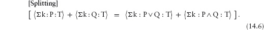
The splitting rule gets its name because it is most often used when P and Q “split” the range into two disjoint sets, that is, when P ∧ Q is everywhere false. In this case, ![]() Σ k:P ∧ Q:T
Σ k:P ∧ Q:T![]() is zero, by the empty-range rule, and may be eliminated from the right side of the rule. Here is the most common example, where we “split” predicate P into P ∧ Qand P ∧ ¬Q.
is zero, by the empty-range rule, and may be eliminated from the right side of the rule. Here is the most common example, where we “split” predicate P into P ∧ Qand P ∧ ¬Q.
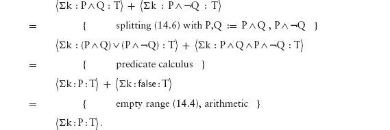
We have thus derived the rule
This rule can now be combined with the one-point rule to split off one term in a summation, as in, for example,
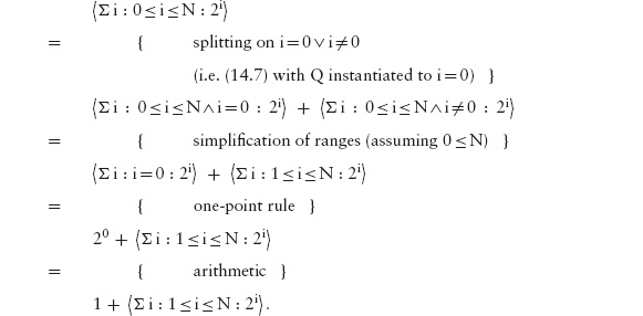
(It is more common to state the splitting rule in the form (14.7). However, the beautiful symmetry of (14.6) makes it more attractive and easier to remember.)
The final rule is a consequence of the rearrangement rule given earlier. It also allows the terms in a summation to be rearranged. Suppose function f maps values of type J to values of type K, and suppose g is a function that maps values of type K to values of type J. Suppose, further, that f and g are inverses. That is, suppose that, for all j∈Jand k∈K,
![]()
Then,
If a function has an inverse, it is called a bijection. The most common use of the translation rule is when the source, J, and target, K, of the function f are the same. A bijection that maps a set to itself simply permutes the elements of the set. So, in this case, (14.8) says that it is permissible to arbitrarily permute the values being added.
The rule is, in fact, a combination of the one-point rule (14.5), the nesting rule (14.2) and the rearrangement rule (14.3); see the exercises at the end of the chapter. We call it the translation rule because, in general, it translates a summation over elements of one type into a summation of elements of another type. It is useful to list it separately, because it is a quite powerful combination of these earlier rules and finds frequent use.
When we use the translation rule, the function f is indicated in the accompanying hint by giving the substitution “k := f(j)”.
Trading Rules The range part of a summation is very convenient to use but, in a formal sense, it is redundant because the information can always be shifted either to the type of the dummy or to the term part. Shifting the information to the type of the dummy is expressed by the rule
Here the type K of the dummy k is replaced by the subset {k∈K | P}. For example, we might consider the natural numbers ![]() to be a subset of the integers
to be a subset of the integers ![]() , specifically {k∈
, specifically {k∈![]() | 0 ≤ k}.
| 0 ≤ k}.
Rule (14.9) is most often used implicitly; in order to avoid specific mention of the range (e.g. if it is not explicitly used in a calculation), the information about the types of the dummies is given in the text and then omitted in the formal quantifications. In this case, the form
![]()
of the notation is used. Formally, ![]() Σk :: T
Σk :: T![]() is a shorthand for
is a shorthand for ![]() Σ k∈K:
Σ k∈K: true :T![]() where K is the declared type of k.
where K is the declared type of k.
Shifting the information in the range to the term part is achieved by exploiting the fact that zero is the unit of addition. For values k not in the given range, we add zero to the sum:
Some texts use a trick peculiar to summation to simplify this rule. The trick is to note that 0×x = 0and 1×x = 1; the boolean value false is mapped to 0 and the boolean value true is mapped to 1. Denoting this mapping by square brackets, the rule reads
![]()
Term Part There are two rules governing the term part. The first allows us to combine two summations over the same range (or, conversely, split up an addition within a summation into two summations):
Like the translation rule, this rule is also a combination of the nesting (14.2) and rearranging rules (14.3) given earlier – because
![]()
It is worth listing separately because it is used very frequently.
The final rule allows us to “factor out” multiplication by a constant from a summation (conversely, it allows us to “distribute” multiplication by a constant into a summation):
The general side condition on the application of rules prohibits the use of distributivity when “k” occurs free in the expression c. (Otherwise, any such occurrences would be released/captured by application of the rule.)
14.2.4 Warning
We conclude this discussion of summation with a warning. Care must be taken when quantifying over an infinite range. In this case, the value of the expression is defined as a limit of a sequence of finite quantifications, and, in some cases, the limit may not exist. For example, ![]() Σ i:0 ≤ i:(−1)i
Σ i:0 ≤ i:(−1)i![]() is not defined because the sequence of finite quantifications
is not defined because the sequence of finite quantifications ![]() Σ i:0 ≤ i < N:(−1)i
Σ i:0 ≤ i < N:(−1)i![]() , for N increasing from 0 onwards, alternates between 0 and 1. So it has no limit. The rules we have given are not always valid when the range of the summation is infinite. The so-called convergence of infinite summations is a well-studied part of mathematics but beyond the scope of this text.
, for N increasing from 0 onwards, alternates between 0 and 1. So it has no limit. The rules we have given are not always valid when the range of the summation is infinite. The so-called convergence of infinite summations is a well-studied part of mathematics but beyond the scope of this text.
14.3 UNIVERSAL AND EXISTENTIAL QUANTIFICATION
Summation is just one example of the quantifiers we want to consider. Readers already familiar with the ![]() notation for continued multiplications will probably have no difficulty rewriting each of the properties of summation into a form that is applicable to multiplication. In general, it is meaningful to “quantify” with respect to any binary operator that is associative and symmetric. As mentioned earlier, addition, multiplication, equivalence, inequivalence, minimum, maximum, conjunction, disjunction, greatest common divisor, and least common multiple are all examples of associative and symmetric operators, and, in each case, it is meaningful (and useful) to consider the operator applied to a number of values rather than just a pair of values.
notation for continued multiplications will probably have no difficulty rewriting each of the properties of summation into a form that is applicable to multiplication. In general, it is meaningful to “quantify” with respect to any binary operator that is associative and symmetric. As mentioned earlier, addition, multiplication, equivalence, inequivalence, minimum, maximum, conjunction, disjunction, greatest common divisor, and least common multiple are all examples of associative and symmetric operators, and, in each case, it is meaningful (and useful) to consider the operator applied to a number of values rather than just a pair of values.
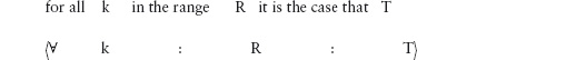
Two quantifications that are particularly important in program specification are so-called universal quantification and existential quantification. Universal quantification extends conjunction to a set of booleans of arbitrary size. Just as for summation, there is a widely accepted symbol denoting universal quantification, namely the “∀” (“for all”) symbol. The notation![]() ∨k:R:T
∨k:R:T![]() means the logical “and” (“∧”) of all values of the boolean expression T determined by assigning to dummy k all values in the range R. In words, it reads
means the logical “and” (“∧”) of all values of the boolean expression T determined by assigning to dummy k all values in the range R. In words, it reads
For example,
![]()
states that the value of the function f is positive for all inputs in the range 0 thru N−1. In dotdotdot notation this is
![]()
When disjunction is extended to an arbitrary set of boolean values, the long-standing mathematical convention is to use the “![]() ” (“there exists”) symbol. The notation
” (“there exists”) symbol. The notation ![]()
![]() k:R:T
k:R:T![]() means the logical “or” (“⋁”) of all values of the boolean expression T determined by assigning to dummy k all values in the range R. In words, it reads
means the logical “or” (“⋁”) of all values of the boolean expression T determined by assigning to dummy k all values in the range R. In words, it reads

For example,
![]()
states that there is some number in the range 0 thru N−1 at which the value of the function f is positive. In dotdotdot notation this is
![]()
14.3.1 Universal Quantification
Just as for summation, we can enumerate a list of rules that govern the algebraic properties of universal and existential quantification. The rules have much the same shape. In this section, we list the rules for universal quantification. Only the splitting rule differs in a non-trivial way from the rules for summation.
The side conditions on application of the rules will not be repeated for individual rules. As a reminder, here, once more, is the statement of the condition.
Side Condition The application of a rule is invalid if it results in the capture of free variables or release of bound variables, or it results in a variable occurring more than once in a list of dummies.
The rules governing the dummies are identical to the rules for summation except for the change of quantifier. The side conditions concerning capture of free variables and/or release of bound variables remain as before.
The rules governing the range are obtained by replacing the quantifier “Σ” by “∀”, replacing “+” by “∧” and replacing 0 (the unit of addition) by true (the unit of conjunction). The proviso on the one-point rule (e contains no occurrences of “k”) still applies.
The empty-range rule (for universal quantification) was apparently a subject of fierce debate among logicians and philosophers when it was first formulated. Algebraically, there can be no dispute: it is a logical consequence of the splitting rule, since P (or Q) can be false.
The splitting rule for universal quantification is simpler than that for summation. The difference is that conjunction is idempotent whereas addition is not. When splitting the range in a universal quantification it does not matter whether some elements of the range are repeated in the two conjuncts. When splitting the range in a summation it does matter whether elements of the range are repeated.
This additional flexibility allows the range in the splitting rule to be generalised from a disjunction P ⋁ Q of two predicates on the dummy to an arbitrary disjunction of predicates on the dummy. That is, we replace an “or” by an existential quantification.
(The side condition on this rule, when used from right to left, demands that “k” is not free in R.)
Trading terms in the range is the same as summation, with the appropriate replacements for the operators and constants. In particular, 0 (the unit of summation) is replaced by true (the unit of conjunction). But, since if P → T ![]() ¬P →
¬P → true fi is thesameas P ⇒T, trading with the term part can be simplified:
The final rules govern the term part. The distributivity law is just one example of a distributivity property governing universal quantification. We see shortly that there are several more distributivity laws.
14.3.2 Existential Quantification
These are the rules for existential quantification. Not surprisingly, they are entirely dual to the rules for universal quantification. (In the rule (14.32), if P → T ![]() ¬P →
¬P → false fi has been simplified to P ∧ T.) Once again, the side condition that free variables may not be captured, and bound variables may not be released, applies to all rules.
14.4 QUANTIFIER RULES
We have now seen four different quantifiers: summation, product, universal quantification and existential quantification. We have also seen that the rules governing the manipulation of these quantifiers have much in common. In this section, we generalise the rules to an arbitrary quantifier. The technical name for the process is abstraction; we “abstract” from particular operators to an arbitrary associative and symmetric operator, which we denote by “![]() ”.
”.
The rules are grouped, as before, into rules for manipulating the dummy, rules for the range part and the term part, and trading rules. The process of abstraction has the added benefit of enabling us to relate different quantifiers, based on distributivity properties of the operators involved. A separate section discussing distributivity has, therefore, also been added.
Warning: In general, the rules given in this section apply only when the range of the quantification is finite. They can all be proved by induction on the size of the range. Fortunately, in the case of universal and existential quantification, this restriction can be safely ignored. In all other cases, it is not safe to ignore the restriction. We have previously mentioned the dangers of infinite summations. An example of a meaningless quantification involving a logical operator is the (associative) equivalence of an infinite sequence of false values (denoted by ![]() ≡ i:0 ≤ i:
≡ i:0 ≤ i: false![]() ). It is undefined because the sequence of finite quantifications
). It is undefined because the sequence of finite quantifications ![]() ≡ i:0 ≤ i < N:
≡ i:0 ≤ i < N: false![]() alternates between
alternates between true and false and has no limit. How to handle infinite quantifications (other than universal and existential quantifications) is beyond the scope of this text.
14.4.1 The Notation
The quantifier notation extends a binary operator, ![]() say, to an arbitrary bag of values, the bag being defined by a function (the term) acting on a set (the range). The form of a quantified expression is
say, to an arbitrary bag of values, the bag being defined by a function (the term) acting on a set (the range). The form of a quantified expression is
![]()
where ![]() is the quantifier, bv is the dummy or bound variable and type is its type, range defines a subset of the type of the dummy over which the dummy ranges, and term defines a function on the range. The value of the quantification is the result of applying the operator
is the quantifier, bv is the dummy or bound variable and type is its type, range defines a subset of the type of the dummy over which the dummy ranges, and term defines a function on the range. The value of the quantification is the result of applying the operator ![]() to all the values generated by evaluating the term at all instances of the dummy in the range.
to all the values generated by evaluating the term at all instances of the dummy in the range.
Strictly, the type of the dummy should always be explicitly stated because the information can be important (as in, for example, the stronger relation between the less-than and at-most orderings on integers compared with their properties on reals). It is, however, information that is often cumbersome to repeat. For this reason, the information is often omitted and a convention on the naming of dummies (such as i, j and k denote integer values) is adopted. This means that the most common use of the notation is in the form
![]()
In addition, the range is sometimes omitted (again to avoid unnecessary repetition in calculations). In this case the form of the quantification is
![]()
and the accompanying text must state clearly what the range is.
As we have defined it, a quantification only has meaning if the operator ![]() is associative and symmetric.1 The operator
is associative and symmetric.1 The operator ![]() should also have a unit in order to make quantification over an empty range meaningful. We denote the unit of
should also have a unit in order to make quantification over an empty range meaningful. We denote the unit of ![]() by
by ![]() .
.
There is often an existing, long-standing, mathematical convention for the choice of the symbol “![]() ” corresponding to the operator
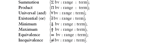
” corresponding to the operator ![]() . If so, we follow that convention. If not we use the same operator symbol, made larger if the printer will allow it. Examples of quantifications are as follows:
. If so, we follow that convention. If not we use the same operator symbol, made larger if the printer will allow it. Examples of quantifications are as follows:
14.4.2 Free and Bound Variables
The notions of “free” and “bound” occurrences of variables were discussed in Section 14.2.2 in the context of summation. The definitions apply to all quantifications, as do the side conditions on the use of rules. (Briefly, capture or release is forbidden, as is repetition of a variable in a list of dummies.) We do not repeat the side conditions below but trust in the reader’s understanding of the concepts.
14.4.3 Dummies
The dummies (or bound variables) in a quantification serve to relate the range and term. There are three rules governing their use:
14.4.4 Range Part
The range part is a boolean-valued expresssion that determines the set of values over which the dummy ranges. There are four rules, two simplification rules and two splitting rules:
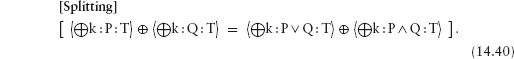
In the case where ![]() is idempotent, the splitting rule can be simplified to
is idempotent, the splitting rule can be simplified to
Furthermore, the right side can be generalised from a disjunction of two propositions P and Q to a disjunction of an arbitrary number (i.e. existential quantification) of propositions. We obtain the following: if ![]() is idempotent,
is idempotent,
14.4.5 Trading
Two trading rules allow information to be traded between the type of the dummy and the range, and between the range and the term part:
14.4.6 Term Part
We give just one rule pertaining to the term part (see also the discussion of distributivity below):
14.4.7 Distributivity Properties
Distributivity properties are very important in mathematical calculations; they are also very important in computations because they are used to reduce the number of calculations that are performed.
A typical distributivity property is the property that negation distributes through addition:
−(x+y) = (−x) + (−y).
The property is used to “factor out” negation, in order to replace subtractions by additions. Similarly, the fact that multiplication distributes through addition,
x×(y+z) = x×y + x×z,
is used to reduce the number of multiplications. Another example is the distributivity of addition through minimum:
x+(y↓z) = (x+y)↓(x+z).
This property is fundamental to finding shortest paths.
Sometimes distributivity properties involve a change in the operator. Multiplication of real numbers is translated into addition, and vice versa, by the rules of logarithms and exponentiation:
ln(x×y) = ln x + ln y,
ex+y = ex × ey.
In words, the logarithm function distributes through multiplication turning it into addition, and exponentiation distributes through addition turning it into multiplication.
It is clear that a distributivity property can be extended from two operands to a finite, non-zero number of operands. We have, for example,
a×(x+y+z) = a×x + a×y + a×z.
Extending a distributivity property to zero operands amounts to requiring that units be preserved. And, by good fortune, that is indeed the case in all the examples given above. Specifically, we have:
−0 = 0 (minus preserves the unit of addition),
x×0 = 0 (multiplying by x preserves the unit of addition),
ln 1 = 0 (the unit of multiplication becomes the unit of addition),
e0 = 1 (the unit of addition becomes the unit of multiplication).
In addition, we can postulate that minimum has a unit ∞ and that
x+∞ = ∞ (addition of x preserves the unit of minimum).
So, in each case, the distributivity property with respect to a binary operator extends to a distributivity property with respect to any finite number of operands, including zero. (The case where there is only one operand is trivial.)
Formally, the general distributivity for quantifications is as follows. Suppose both ![]() and ⊗ are associative and symmetric operators, with units
and ⊗ are associative and symmetric operators, with units ![]() and 1⊗, respectively. Suppose f is a function with the properties that
and 1⊗, respectively. Suppose f is a function with the properties that
![]()
and, for all x and y,
![]()
Then
An important example of the distributivity law is given by the so-called De Morgan’s rules for universal and existential quantification. De Morgan’s rules for binary conjunctions and disjunctions were given in Section 13.4. In words, logical negation distributes through disjunction, turning it into conjunction; logical negation also distributes through conjunction, turning it into disjunction. But, since ¬false is true and ¬true is false, the binary rule extends to an arbitrary existential or universal quantification:
The warning about existence of summations over an infinite range does not apply to universal or existential quantifications. Any universal or existential quantification you care to write down has meaning and the above rules apply.
14.5 EXERCISES
1. Evaluate the following summations.
(a) ![]() Σ k : 1 ≤ k ≤ 3 : k
Σ k : 1 ≤ k ≤ 3 : k![]()
(b) ![]() Σ k : 0 ≤ k < 5 : 1
Σ k : 0 ≤ k < 5 : 1![]()
(c) ![]() Σ i,j : 0 ≤ i < j ≤ 2 ⋀ odd(i) : i+j
Σ i,j : 0 ≤ i < j ≤ 2 ⋀ odd(i) : i+j![]()
(d) ![]() Σ i,j : 0 ≤ i < j ≤ 2 ⋀ odd(i) ⋀ odd(j) : i+j
Σ i,j : 0 ≤ i < j ≤ 2 ⋀ odd(i) ⋀ odd(j) : i+j![]()
2. What is the value of ![]() Σ k:k2 = 4:k2
Σ k:k2 = 4:k2![]() in thecasewhere the type of k is
in thecasewhere the type of k is
(a) a natural number,
(b) an integer?
3. Identify all occurrences of free variables in the following expressions.
(a) 4 × i
(b) ![]() Σ j:1 ≤ j ≤ 3:4×i
Σ j:1 ≤ j ≤ 3:4×i![]()
(d) ![]() Σ j:1 ≤ j ≤ 3:m×j
Σ j:1 ≤ j ≤ 3:m×j![]() +
+ ![]() Σ j:1 ≤ j ≤ 3:n×j
Σ j:1 ≤ j ≤ 3:n×j![]()
(e) ![]() Σ j:1 ≤ j ≤ 3:m×j
Σ j:1 ≤ j ≤ 3:m×j![]() +
+ ![]() Σ k:1 ≤ k ≤ 3:n×j
Σ k:1 ≤ k ≤ 3:n×j![]()
4. Evaluate the left and right sides of the following equations. Hence, state which are everywhere true and which are sometimes false.
(a) ![]() Σ j:1 ≤ j ≤ 3:4×i
Σ j:1 ≤ j ≤ 3:4×i![]() =
= ![]() Σ k:1 ≤ k ≤ 3:4×i
Σ k:1 ≤ k ≤ 3:4×i![]()
(b) ![]() Σ j:1 ≤ j ≤ 3:4×j
Σ j:1 ≤ j ≤ 3:4×j ![]() =
= ![]() Σ k:1 ≤ k ≤ 3:4×j
Σ k:1 ≤ k ≤ 3:4×j![]()
(c) ![]() Σ j: 1 ≤ j ≤ 3:
Σ j: 1 ≤ j ≤ 3: ![]() Σ k:k = 0:4×j
Σ k:k = 0:4×j![]()
![]()
= ![]() Σ i:1 ≤ i ≤ 3:
Σ i:1 ≤ i ≤ 3: ![]() Σ k:k = 0:4×i
Σ k:k = 0:4×i![]()
![]()
(d) ![]() Σ j: 1 ≤ j ≤ 3:
Σ j: 1 ≤ j ≤ 3: ![]() Σ j:j = 1:4×j
Σ j:j = 1:4×j![]()
![]()
= ![]() Σ k:1 ≤ k ≤ 3:
Σ k:1 ≤ k ≤ 3: ![]() Σ j:j = 1:4×k
Σ j:j = 1:4×k![]()
![]()
5. Derive the trading rule (14.10) from the splitting rule (14.6). You may assume that ![]() Σ k:R:0
Σ k:R:0![]() = 0 for all ranges R.
= 0 for all ranges R.
6. Derive (14.8) from the one-point rule (14.5), the nesting rule (14.2) and the rearrangement rule (14.3). Hint: your derivation should head for using the fact thatf is a bijection, that is, that there is a function g such that, for all j∈J and k∈K,
f(j) = k ≡ j = g(k).
Use the one-point rule to introduce a second dummy so that you can exploit this property.
7. Prove the generalised distributivity law![]()
What are the side conditions on using this rule?
8. Derive the rule![]()
Use this rule to derive (14.41) from (14.40) in the case where ![]() is idempotent.
is idempotent.
9. The translation rule for summations (14.8) requires function f to be a bijection. The rule is applicable to all quantifications, and not just summations.
In the case where the quantifier is idempotent, the rule can be simplified. The translation rule for idempotent quantifiers is as follows. Suppose f is a function from the type of dummy j to the type of dummy k such that
![]()
Then![]()
Prove this rule.
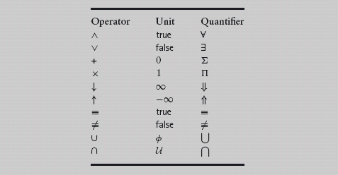
10. The following table shows a number of associative and symmetric binary operators together with their units. For each, give an instance of the distributivity rule (14.46) not already mentioned in the text.
1This assumption can be avoided if an order is specified for enumerating the elements of the range – this is what is done in so-called “list comprehensions” in functional programming languages. The rules on nesting and rearrangement would then no longer apply.