

In Section 12.7, we showed how binary relations can be depicted as graphs. In this chapter, we discuss the connection between relations and graphs in more detail. Many algorithmic problems involve finding and/or evaluating paths through a graph. Our goal in this chapter is to show how these problems are represented algebraically so that the solution to such tasks can be calculated.
16.1 PATHS IN A DIRECTED GRAPH
We begin the chapter with a number of formal definitions about graphs and paths in a graph. Informally, the notions we introduce are easy to grasp. So, on a first reading, it is not essential to pay attention to the details of the definitions. The details are essential later, when the definitions are used in earnest.
Definition 16.1 (Directed Graph) A directed graph comprises two sets N and E, called the nodes and the edges of the graph, and two functions from and to, both of which have type E→N.
If e is an edge of a graph and from(e) = m and to(e) = n (where m and n are nodes of the graph), we say that e is an edge from node m to node n.
We sometimes write statements of the form “let G = (N,E,from,to)” as a shorthand for introducing a graph and giving it the name G.
Very often, the graphs we consider have a finite set of nodes and a finite set of edges. Later, we also consider labelled graphs. A labelling of a graph is a function defined on the edges of the graph. The labels (the values taken by the function) may be booleans, in which case the function has type E→Bool, or numbers, in which case the function has type E→IN, or indeed any type that is relevant to the problem in hand.
If the sets of nodes and edges are sufficiently small, it can be informative to draw a picture of a graph. Figure 16.1 shows how we depict a labelled edge in a graph from a node called fee to a node called foo with label fum. Note how the arrowhead indicates the values of the functions from and to when applied to the edge. Sometimes, if there is no need to name the nodes, we draw them as small black dots.

![]() Figure 16.1: A labelled edge.
Figure 16.1: A labelled edge.
The definition of a graph allows multiple edges with the same from and to nodes. This is an aspect of the definition that we do not exploit. Generally, for any pair of nodes m and n, we assume that there is at most one edge from m to n.
Often we talk about “graphs” instead of “directed” graphs. A directed graph can be thought of as a communication network where all communication is one-way, in the direction indicated by the arrows. Sometimes it is more appropriate to use “undirected” graphs, which can be thought of as communication networks where communication is always two-way and entirely symmetric.
Definition 16.2 (Undirected Graph) An undirected graph comprises two sets N and E, called the nodes and the edges of the graph, and a function endpts with domain E. The function endpts is such that, for each edge e, the value of endpts(e) is a bag of nodes of size 2.
The name “endpts” is short for “end-points”. That endpts(e) is a bag of size 2 means that it may have two distinct elements, or just one element repeated twice. In the latter case, the edge is called a self-loop. Figure 16.2 depicts an undirected graph with two (unnamed) nodes and two edges, one of which is a self-loop. Just as for directed graphs, although the definition allows the possibility of multiple edges with the same end-points, we generally assume that there is at most one edge between any pair of end-points.
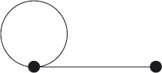
![]() Figure 16.2: An undirected graph with two nodes and two edges.
Figure 16.2: An undirected graph with two nodes and two edges.
Clearly, an undirected graph can be converted into a directed graph. An edge e with distinct end-points m and n is converted into two edges e1 and e2 with m and n as their from and to nodes but in opposite directions. A self-loop is converted into a single edge where the from and to nodes are equal.1 We often omit the adjectives “directed” or “undirected” when it is clear from the context which is meant.
Many problems are modelled as searching paths through a graph. Here is the definition of a “path”.
Definition 16.3 (Path) Suppose (N, E, from, to) is a graph and suppose s and t are nodes of the graph. A path from s to t of edge-count k is a sequence of length 2k + 1 of alternating nodes and edges; the sequence begins with s and ends with t, and each subsequence of the form m, e, n where m and n are nodes and e is an edge has the property that from(e) = m ∧ to(e) = n. The nodes s and t are called the start and finish nodes of the path.
Figure 16.3 depicts a path of edge-count 3 from node start to node finish. Formally, the path is the sequence
start, e1, n1, e2, n2, e3, finish.

![]() Figure 16.3: A path of edge-count 3.
Figure 16.3: A path of edge-count 3.
It is important to note that the definition of a path allows the edge-count to be 0. Indeed, there is a path of edge-count 0 from every node in a graph to itself: a sequence of length 1 consisting of the node s satisfies the definition of a path from s to itself. Such a path is called an empty path. Note also that edge e defines the path
from(e), e, to(e)
of edge-count 1.
Edges and paths have different types and should not be confused. Even so, it is sometimes convenient not to make the distinction between edges and paths of edge-count 1. However, a self-loop on a node should never be confused with the path of edge-count 0 from the node to itself: a self-loop defines a path of edge-count 1 from the node to itself.
Paths are sometimes represented by sequences of nodes, omitting explicit mention of the connecting edges. (We use such a representation in Section 16.4.4.) Paths may also be represented by sequences of edges, omitting explicit mention of the nodes (e.g. where there may be more than one edge connecting a given pair of nodes and the distinction between edges is important.) This is unproblematic except for the case of empty paths, where the representation is ambiguous: the empty sequence of edges does not identify the start/finish node of the path.
Definition 16.4 (Simple Paths and Cycles) A path in a graph is said to be simple if no node is repeated. A path of edge-count at least 1 with the same start and finish nodes is called a cycle. A graph is said to be acyclic if it has no cycles.
16.2 GRAPHS AND RELATIONS
We first introduced graphs in Section 12.7 as a way of picturing binary relations. We introduced Hasse diagrams in Section 12.7.6 as an economical way of presenting the transitive closure of a relation because it is easy for us to see paths through the graph. In this section, we explore in more detail the correspondence between relations and graphs.
Recall that a binary relation is a function of two arguments that is boolean-valued. Recall also that sets and boolean-valued functions are “isomorphic”. That is, a boolean function defines a set (the set of all values for which the value of the function is true) and, vice versa, a set defines a boolean function on values via membership (each value is either a member of the set or not). Applied to relations, this means that a binary relation can be defined to be a set; if the types of its arguments are A and B, a relation is a subset of A×B. In other words, a binary relation on A and B is a set of pairs (a, b) where a is an element of A and b is an element of B. When the sets A and B are very small, this set-oriented view of relations can be easier to work with. This is the case for the examples we present in this section. Our practice is to switch between the two views of relations, choosing the set-oriented or the boolean-valued-function view as appropriate.
The examples of relations in Section 12.7 were all of so-called homogeneous relations, that is, relations where the types A and B are the same. Homogeneous relations are of most interest, but let us consider so-called heterogeneous relations, that is, relations where A and B may be different.
Let us begin with an example. We start with just two sets: {a,b,c} with three elements and {j,k} with two elements. The cartesian product {a,b,c}×{j,k} has 3×2 (i.e. 6) elements. A relation between {a,b,c} and {j,k} is a subset of {a,b,c}×{j,k}. There are 26 (i.e. 64) such relations because there are 2 possibilities for each of the 6 elements of {a,b,c}×{j,k}: each is either an element of or not an element of the relation. Since the number of elements in each relation is at most 6, we can specify each relation just by listing its elements. Indeed, we can draw a picture depicting each relation.
Figure 16.4 depicts one such relation. Viewing relations as sets, it is
{(a, j), (b, k), (c, j), (c, k)}.
Viewing relations as boolean-valued functions, it is the function that maps the pairs (a, j), (b, k), (c, j) and (c, k) to true and the pairs (a, k) and (b, j) to false. In words, we would say that a is related to j, b is related to k, and c is related to j and k. Figure 16.4 depicts the relation as a graph in which the nodes are the elements of the set {a,b,c} ∪ {j,k} and there is an edge from an element of {a,b,c} to an element of {j,k} when the pair of elements are related.
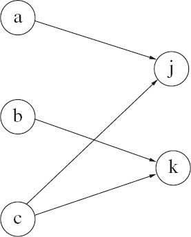
![]() Figure 16.4: Bipartite graph depicting the relation {(
Figure 16.4: Bipartite graph depicting the relation {(a, j), (b, k), (c, j), (c, k)}.
For arbitrary sets A and B, a subset of A×B is said to be a (heterogeneous) relation of type A∼B. This defines “∼” as a type former which combines cartesian product and power sets; indeed, A∼B is an alternative notation for 2A×B, the set of subsets of A×B. Figure 16.4 depicts a relation of type {a,b,c} ∼ {j,k}.
The graph in Figure 16.4 is called a bipartite graph because the nodes of the graph can be split into two disjoint sets such that all edges are from nodes in one of the sets to nodes in the other set. It is bipartite for the simple reason that it models a relation of type A∼B for which A and B are disjoint sets. When the sets A and B are not disjoint and we model a heterogeneous relation of type A∼B as a graph, we lose type information: we view it as a homogeneous relation on the set A∪B. The distinction is sometimes important – it first becomes important for us when we introduce matrices in Section 16.5 – but often it can be ignored. Nevertheless, for greater clarity our initial examples are all of relations of type A∼B where A and B are indeed disjoint.
16.2.1 Relation Composition
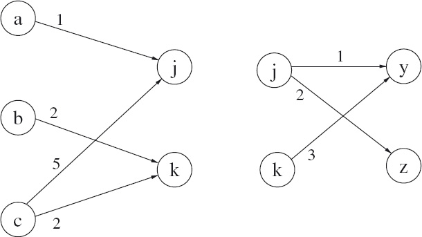
In Figure 16.5, the same relation is depicted together with a second relation. The second relation is a relation, {(j, y), (j, z), (k, y)}, of type {j,k} ∼ {y,z}. A relation of type A∼B can be composed with a relation of type B∼C; the result is a relation of type A∼C. The result of composing the two relations in Figure 16.5 is depicted in Figure 16.6. Let us explain how the graph in Figure 16.6 is constructed from the two graphs in Figure 16.5. Afterwards we give a precise definition of the composition of two relations.
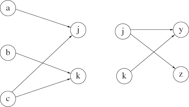
![]() Figure 16.5: Graphs depicting two relations that can be composed.
Figure 16.5: Graphs depicting two relations that can be composed.

![]() Figure 16.6: Graph depicting the composition of the two relations in Figure 16.5.
Figure 16.6: Graph depicting the composition of the two relations in Figure 16.5.
Essentially the process is to replace two connecting edges by one edge. For example, in Figure 16.5 there is an edge in the left graph from a to j and an edge in the right graph from j to y; this results in an edge from a to y in Figure 16.6. Similarly, there is an edge from b to y resulting from the two connecting edges from b to k and from k to y. But there is a complication. Note that there is only one edge from c to y but there are two ways that the edge arises: both nodes j and k act as connecting nodes.
An edge in the graph shown in Figure 16.6 corresponds to the existence of at least one path formed by an edge in the left graph of Figure 16.5 followed by an edge in the right graph of Figure 16.5; two such edges form a path if they are connected, that is, they have an intermediate node in common.
Retracing our steps, the two graphs in Figure 16.5 depict two relations, the first of type {a,b,c}∼{j,k} and the second of type {j,k}∼{y,z}. The two relations can be composed and their composition is depicted by the graph in Figure 16.6. Formally, suppose R is a relation of type A∼B and S is a relation of type B∼C. Then their composition, which we denote by R◦S, is the relation of type A∼C defined by:
Definition (16.5) views relations as sets of pairs. If we take the view that a relation is a boolean-valued function, we would write a R b instead of (a, b)∈R. In that case, the definition would be formulated as:
Having introduced a binary operator on relations, it is important to investigate its algebraic properties. Composition is easily shown to be associative. Specifically, if A, B, C and D are types and R, S and T are relations of type A∼B, B∼C and C∼D, R◦(S◦T) and (R◦S)◦T are equal relations of type A∼D. The proof is a straightforward calculation. Here is an outline:
a (R◦(S◦T)) d
= { expand the definition of composition twice;
apply distributivity of conjunction over disjunction
and idempotence of conjunction }
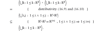
![]() ∃ b,c : b∈B∧c∈C : (aRb) ∧ (b S c) ∧ (c T d)
∃ b,c : b∈B∧c∈C : (aRb) ∧ (b S c) ∧ (c T d)![]()
= { same steps but applied to (R◦S)◦T
and reversed }
a ((R◦S)◦T) d.
then follows by the rule of extensionality (two functions are equal if they always return equal values). As a consequence, we may omit parentheses and write simply R◦S◦T.
Note how relation composition is defined in terms of conjunction and disjunction; it is thus the algebraic properties of these two logical operators that are the key to the properties of composition. Note also how the middle formula of the skeleton calculation above expresses that a and d are related by R◦S◦T if there is a path in the graphs for R, S and T beginning with an edge in the graph for R followed by an edge in the graph for S and ending with an edge in the graph for T; associativity of composition captures the property that the order in which the edges are combined to form a path is not significant.
Relation composition is not symmetric. Indeed, for heterogeneous relations it does not usually make sense to swap the order of composition. For homogeneous relations – relations R and S both of type A∼A for some A – the equality R◦S = S◦R makes sense but is sometimes true and sometimes false. Oviously, it is true when R=S. For an example of when it is false, take A = {a,b,c}, R = {(a,b)} and S = {(b,c)}. Then R◦S = {(a,c)} and S◦R = ![]() . Thinking in terms of paths in a graph, it is obvious that the order of the edges is important.
. Thinking in terms of paths in a graph, it is obvious that the order of the edges is important.
Note that we have just used our standard notation “![]() ” for the empty set. Strictly, because relations are typed, we should distinguish between different “types” of empty set, as in
” for the empty set. Strictly, because relations are typed, we should distinguish between different “types” of empty set, as in ![]() A∼A. This is not usually done, the context being used to determine which relation is meant. In the context of relations, it is usual to call
A∼A. This is not usually done, the context being used to determine which relation is meant. In the context of relations, it is usual to call ![]() the empty relation and sometimes a different symbol is chosen. For reasons explained in Section 16.4, we use the symbol 0 for the empty relation (the type being either evident from the context or left to the reader to infer).
the empty relation and sometimes a different symbol is chosen. For reasons explained in Section 16.4, we use the symbol 0 for the empty relation (the type being either evident from the context or left to the reader to infer).
The empty relation (of appropriate type) is the left and right zero of composition. That is, for all relations R,
(Typically, all three occurrences of “0” in this law have different type, but that is not important.)
16.2.2 Union of Relations
Union is defined on all sets and so also on relations, the only proviso being that the relations being combined have the same type. That is, if R and S both have the same type, A∼B say, then R∪S is a relation also of type A∼B. The union of relations is symmetric, associative, idempotent and has unit 0 (the empty relation).
The set A×B is a subset of A×B – after all, the two are equal – and so is a relation of type A∼B. It is called the universal relation of its type because it relates every element of A to every element of B. It is interesting because it is the zero of the union of relations of type A∼B: with R ranging over relations of type A∼B, we have
[ (A×B) ∪ R = A×B ] .
This is a simple consequence of the fact that R is a relation of type A∼B is, by definition, R ⊆ A×B.
If we depict relations of type A∼B as bipartite graphs, union corresponds to choice: there is an edge in the graph of R∪S from a to b if there is an edge in the graph of R from a to b or there is an edge in the graph of S from a to b. An expression like (R∪S)◦T captures paths formed by a choice of edge in R or S followed by an edge in T. The expression R◦T ∪ S◦T is similar; it captures paths formed by either an edge in R followed by an edge in T or an edge in S followed by an edge in T. Indeed, the two are equal; composition distributes over union. That is, if R and S both have type A∼B and T has type B∼C, for some A, B and C, we have
Similarly, if R has type A∼B and S and T have type B∼C, for some A, B and C,
An immediate consequence of distributivity is that composition is monotonic. Specifically, if R has type A∼B and S and T have type B∼C, for some A, B and C,
and, if S and T have type A∼B and R has type B∼C, for some A, B and C,
The following calculation establishes (16.11):
R◦S ⊆ R◦T
= { definition of ⊆ }
(R◦S) ∪ (R◦T) = R◦T
= { distributivity: (16.9) }
R◦(S∪T) = R◦T
![]() { Leibniz }
{ Leibniz }
S∪T = T
= { definition of ⊆ }
S ⊆ T.
16.2.3 Transitive Closure
In a bipartite graph of type A∼B, edges are from nodes in A to nodes in B; in an arbitrary graph, there is no restriction on the edges. Such graphs correspond to homogeneous relations, that is, relations of type A∼A for some A. Indeed, every relation R of type A∼A defines a graph with node-set A and an edge from node a to node a′ whenever a R a′. Conversely, given a graph (A,E,from,to), we can define a relation R of type A∼A by a R a′ exactly when there is an edge from a to a′ in E.
In this section, we fix the set A and consider relations of type A∼A. This has the enormous advantage that we do not have to continually mention types or type restrictions. Composition and union are well defined on all relations and there is no ambiguity about using 0 to denote the empty relation. The set A does not go away; it becomes an implicit parameter in all definitions.
Our goal in this section is to show that computing the transitive closure of a relation is the same as establishing the existence of paths (of edge-count at least 1) in the graph of the relation.
Recall that a relation R is transitive if, for all x, y and z, whenever x R y is true, and y R z is true, it is also the case that x R z is true. In the following calculation, we express this property in terms of relation composition:
R is transitive
= { definition }
![]() ∀ x,y,z : x R y ∧ y R z : x R z
∀ x,y,z : x R y ∧ y R z : x R z![]()
= { range splitting }
![]() ∀ x,z :
∀ x,z : ![]() ∃y :: x R y ∧ y R z
∃y :: x R y ∧ y R z![]() : x R z
: x R z![]()
= { definition of composition: (16.6) }
![]() ∀ x,z : x (R◦R) z : x R z
∀ x,z : x (R◦R) z : x R z![]() .
.
Taking the set-oriented view of relations, the universal quantification
![]() ∀ x,z : x (R◦R) z : xRz
∀ x,z : x (R◦R) z : xRz![]()
equivales
R◦R ⊆ R.
In this way, we have established the so-called point-free definition of transitivity:
(It is called “point-free” because the “points” x, y and z do not appear in the definition.)
Now let us turn to paths in a graph. The occurrence of “R◦R” in definition (16.13) suggests that we consider its graphical representation. We determined in Section 16.2.1 that values related by S◦T correspond to nodes that are connected by a path consisting of an edge in the graph of S followed by an edge in the graph of T. Although Section 16.2.1 restricted graphs to bipartite graphs, the restriction was not essential. Indeed, values related by R◦R correspond to paths in the graph of R of edge-count 2.
A generalisation is obvious. Suppose we write R1 for R, R2 for R◦R, R3 for R◦R◦R, and so on. Then Rk (for all strictly positive2 natural numbers k) corresponds to paths in the graph of R of edge-count k. This is exemplified in the graphs in Figure 16.7. The top graph depicts a relation R on a set of size 5. The middle graph depicts R2 and the bottom graph depicts R3. An edge in the middle graph corresponds to a path in the top graph of edge-count 2 and an edge in the bottom graph corresponds to a path in the top graph of edge-count 3.
Set union expresses a choice among relations and, hence, a choice among edge-counts. For example, the graph of the relation
![]()
expresses a choice of paths in the graph of R with edge-count 1, 2 or 3. The graph of the relation
expresses a choice among all paths of edge-count at least 1 in the graph of R. We show shortly that this is the transitive closure R+ of R.
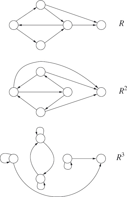
![]() Figure 16.7: First, second and third powers of a relation.
Figure 16.7: First, second and third powers of a relation.
Although (16.14) is a quantification with an infinite range and we have warned that the rules for manipulating quantified expressions do not necessarily apply in such cases, the quantification can always be reduced to a finite range if the domain of the relation R is finite. This is easy to see from the correspondence with paths in a graph. If the number of nodes in a graph is a finite number, n, and there is a path from one node to another in the graph, then there must be a path of edge-count at most n. This is because every path can always be reduced to a simple path by removing proper subpaths that start and finish at the same node; clearly, a simple path comprises at most n edges. (See Definition 16.4 for the precise definition of “simple”.)
In order to show that (16.14) is indeed the transitive closure R+ of R, we need a concise definition of transitive closure. A point-free definition is the most concise.
The definition has two clauses. First, R+ is transitive:
Second, R+ is the least relation (in the subset ordering) that includes R and is transitive. Formally:
Our goal is to establish the law
To do this, we have to show that properties (16.15) and (16.16) are satisfied when R+ is replaced by ![]() That is, we have to show that
That is, we have to show that
and
We begin with the transitivity requirement:
This proves (16.18). Now we establish the “least” requirement. We begin with the more complicated side of the equivalence in (16.19) and try to prove it equal to the left side. On the way we discover that a proof by mutual implication is necessary.
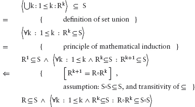

Noting that this calculation begins and ends with the right side of (16.19), and the left side is the penultimate expression, we conclude (16.19) by the rule of mutual implication.
16.2.4 Reflexive Transitive Closure
The reflexive transitive closure of a (homogeneous) relation R is denoted by R*. It is defined similarly to the transitive closure. In words, it is the least reflexive and transitive relation that includes R.
In order to give it a compact, point-free definition, we need to express reflexivity in a point-free way. Recall that R is reflexive if x R x for all x. Let us define the relation 1 by
![]() ∀ x,y :: x 1 y ≡ x = y
∀ x,y :: x 1 y ≡ x = y![]() .
.
Then we have:
R is reflexive
= { definition }
![]() ∀x :: x R x
∀x :: x R x![]()
= { one-point rule }
![]() ∀ x,y : x = y : x R y
∀ x,y : x = y : x R y![]()
= { definition of 1, Leibniz }
![]() ∀ x,y : x 1 y : x R y
∀ x,y : x 1 y : x R y![]()
= { definition of subset }
1 ⊆ R.
The relation 1 is called the identity relation and sometimes denoted by id (or Id). We choose to use the symbol 1 here because the identity relation is the (left and right) unit of composition. That is,
On account of the unit law, it is appropriate to define
![]()
then we have the familiar-looking law of powers
![]()
where m and n are arbitrary natural numbers.
We can now give a definition of reflexive transitive closure. First, R* is reflexive and transitive:
Second, R* is the least relation (in the subset ordering) that includes R and is reflexive and transitive. Formally:
The graph of 1 has a self-loop on every node (an edge from every node to itself) and no other edges. For any given graph, it represents the paths of edge-count 0. The graph of the reflexive transitive closure of R has an edge for every path, including paths of edge-count 0, in the graph of R. Formally:
(Note the inclusion of 0 = k in the quantified expression.) The proof of this law is almost a repetition of the proof of the law (16.17).
Laws (16.17) and (16.23) are the mathematical basis for the use of Hasse diagrams to depict ordering relations and the use of genealogy trees to depict ancestral relations. More broadly, we exploit these laws every time a graph is used to depict a network of points with connecting lines. The information content of the diagram is kept to a minimum while we rely on our ability to trace paths in order to deduce required information from the graph. Even for problems where the graph is too big to display, the laws form the basis for many search algorithms. The transitive closure and reflexive transitive closure operations on relations/graphs are thus very important concepts.
16.3 FUNCTIONAL AND TOTAL RELATIONS
Functions are relations that relate exactly one output to each and every input value. This section makes this precise.
First, let us note that relations are ambivalent about “input” and “output”. That is, given a relation R of type A∼B, we may choose arbitrarily whether we regard A to be the set of “inputs” and B the set of “outputs” or, vice versa, B to be the set of “inputs” and A the set of “outputs”. Because it fits better with conventional notations for the composition of relations and functions, we choose to call B the input set and A the output set.
We say that R is functional (on B) if, for all x, y in A and for all z in B, if x R z and y R z then x = y. (In words, R returns at most one “output” for each “input” value.) We also say that R is total (on B) if, for all z in B, there is some x in A such that x R z. (In other words, R returns at least one “output” for each “input” value.) We say that the relation R of type A∼B is a function to A from B if R is both functional and total on B. If this is the case, we write R(z) for the unique value in A that is related by R to z.
The converse of relation R of type A∼B, which we denote by R∪, has type B∼A. If R∪ is functional on A, we say that R is injective. If R∪ is total on B, we say that R is surjective. A relation R of type A∼B is a bijective function if R is a function to A from B and R∪ is a function to B from A. “Bijective function” is commonly abbreviated to “bijection”. If there is a bijection of type A∼B, we say that sets A and B are in one-to-one correspondence. For example, the doubling function is a bijection that defines a one-to-one correspondence between the natural numbers and the even natural numbers.
When the definitions of functionality and injectivity, totality and surjectivity are expressed in a point-free fashion, the duality between them becomes very clear. Using the notations 1A and 1B for the identity relations on A and B, respectively, we have:
If f and g are functional relations of type A∼B and B∼C, respectively, their composition f◦g is a functional relation of type A∼C. We say that functionality is preserved by composition. Similarly, totality, injectivity and surjectivity are all preserved by composition. In particular, the composition of a function f of type B→A (a total, functional relation of type A∼B) and a function g of type C→B (a total, functional relation of type B∼C) is a function f◦g of type C→A. Given input z, the unique value related to z by f◦g is f(g(z)).
16.4 PATH - FINDING PROBLEMS
In this section, we look at different applications of graph theory that can all be described under the general heading of “path-finding problems”. At the same time, our goal is to formulate the mathematical structure of such problems. To this end, we introduce product and sum operations on labelled graphs. The definition of “product” and “sum” depends on the application; the mathematical structure binds the applications together.
16.4.1 Counting Paths
In Section 16.2 the focus was on boolean values: whether or not two nodes in a graph are related by the existence of a path connecting them. Suppose now that we would like to determine in how many ways two nodes are connected. Then we need to redefine the way graphs are composed.
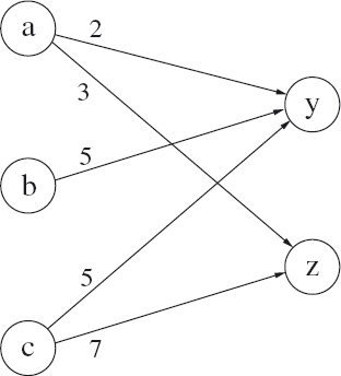
To better illustrate the technique, Figure 16.8 shows the same two graphs as in Figure 16.5 but now each edge has been labelled with a number. For example, the edge from c to k in the left graph has label 2. Let us interpret this as meaning that there are in fact two different edges from c to k. Similarly, the label 5 on the edge from c to j means that there are actually five edges from c to j. Where there is no edge (for example, there is no edge from node b to node j in the left graph), we could equally have drawn an edge with label 0. Now suppose we want to determine the number of different paths from each of the nodes a, b and c to each of the nodes y and z in the combined graph. There are six different combinations. Let us consider each combination in turn.
![]() Figure 16.8: Two labelled graphs that can be connected.
Figure 16.8: Two labelled graphs that can be connected.
From a to y there is just one path, because there is one edge from a to j and one edge from j to y, and j is the only connecting node. From a to z there are 1×2 paths because, again, j is the only connecting node, and there is one edge from a to j and there are two edges from j to z.
From b to y, there are 2×3 paths because a path consists of one of the 2 edges from b to k followed by one of the 3 edges from k to y.
From c to y there is a choice of connecting node. There are 5×1 paths from c to y via the connecting node j; there are also 2×3 paths from c to y via the connecting node k. In total, there are thus 5×1 + 2×3 paths from c to y. Finally, there are 5×2 paths from c to z.

![]() Figure 16.9: Result of counting paths: the standard product.
Figure 16.9: Result of counting paths: the standard product.
Figure 16.9 shows the result of this calculation. Note that 1 (the number of paths from a to y) equals 1×1 + 0×0, 2 (the number of paths from a to z) equals 1×2 + 0×0, 6 (the number of paths from b to y) equals 2×3 + 0×0, and 10 (the number of paths from c to z) equals 5×2 + 0×0. Moreover, 0 (the number of paths from b to z) equals 0×0 + 0×0. In this way, there is a systematic method of computing the number of paths for each pair of nodes whereby “+” corresponds to a choice of connecting node and “×” corresponds to combining connecting edges.
Let us fomalise this method. We begin by overloading the notation introduced earlier for describing the types of relations. We say that G is a bipartite graph of type A∼B if A∪B is the set of vertices of G and each edge of G is from a node in A to a node in B. If the edges of bipartite graphs G and H are labelled with numbers, and G has type A∼B and H has type B∼C (for some A, B and C), the (standard) product G×H is a bipartite graph of type A∼C; writing a G b for the label given to the edge from a to b, the labels of edges of G×H are given by
Note that (16.29) assumes that, for each pair of nodes, no edge connecting them is the same as an edge that does connect them but with label 0. The reason for naming this combination of G and H a “product” will become clear in Section 16.4.5.
16.4.2 Frequencies
Figure 16.10 shows our two example graphs again but this time the edge labels are ratios of the form m/n. Imagine that the nodes of the graphs represent places and the edges represent routes connecting the places. The two graphs might represent different modes of transport. For example, the left graph might represent bicycle routes and the right graph bus routes. A person might complete the first part of a journey by bicycle and then the second part by bus. The labels represent the frequency with which a particular route is chosen. For example, a person starting at c might follow the route to j one time in every three and the route to k twice. Note that, for the labels to make sense in this way, the labels on the edges from each node must add up to 1. Indeed, this is the case for node c (since ![]() ). Since there is only one edge from node
). Since there is only one edge from node a, the edge has to be labelled ![]() . Note, however, that the sum of the edge labels for edges to a given node do not have to add up to 1. For example, the edge labels on the edges into node
. Note, however, that the sum of the edge labels for edges to a given node do not have to add up to 1. For example, the edge labels on the edges into node j add up to ![]() .
.

![]() Figure 16.10: Frequency labellings.
Figure 16.10: Frequency labellings.
A question we might ask is with what frequency a person takes a particular (bicycle followed by bus) route. Since the question is very similar to counting paths, it is not surprising that the method is to add products of frequencies according to the formula (16.29). Let us see how this works for node c.
Referring to Figure 16.10, since 6 is the least common multiple of 2 and 3, we consider 6 trips starting from c. Of these, 6×![]() (i.e. 2) will be made to node j, from where 6×
(i.e. 2) will be made to node j, from where 6×![]() ×
×![]() will proceed to node
will proceed to node y. Simplifying, 1 of the 6 trips will be made from c to y via node j. Similarly, 6×![]() ×
×![]() (i.e. 4) of the trips will be made from
(i.e. 4) of the trips will be made from c to y via node k. In total, 1+4 (i.e. 5) out of 6 trips from c will be to y. Also, 6×![]() ×
×![]() (i.e. 1) out of 6 trips will be made from
(i.e. 1) out of 6 trips will be made from c to z. Note that ![]() , meaning that all 6 of the 6 trips are made to either
, meaning that all 6 of the 6 trips are made to either y or z.

![]() Figure 16.11: Frequency count: the standard product of the graphs in Figure 16.10.
Figure 16.11: Frequency count: the standard product of the graphs in Figure 16.10.
Figure 16.11 shows the result of calculating the frequencies for each of the nodes in the left graph. The formula used to calculate frequencies is precisely the same formula (16.29) used to count paths. As remarked earlier, this is not surprising: if all the labels are ratios of positive integers, and m is the least common multiple of all the denominators (the denominator of ![]() is q), then multiplying each label by m gives a count of the number of times the edge is followed in every m times that a path is traversed.
is q), then multiplying each label by m gives a count of the number of times the edge is followed in every m times that a path is traversed.
16.4.3 Shortest Distances
Let us return to Figure 16.8. In Section 16.4.1 we viewed the labels on the edges as counts. So, for example, the label 2 on the edge from c to k was taken to mean the existence of two different edges from c to k. Let us now view the labels differently. Suppose the nodes represent places and the labels represent distances between the places. So the label 2 on the edge from c to k means that the two places c and k are connected by a (one-way) path of length 2. The question is: if the paths from a, b and c via j and k to y and z are followed, what is the shortest distance that is travelled?
The analysis is almost the same as for counting paths. From a to y the distance is 1+1 (i.e. 2) because there is one edge from a to j of length 1 and one edge from j to y, also of length 1, and j is the only connecting node. From a to z the distance is 1+2 because, again, j is the only connecting node, and the edge from a to j has length 1 and the edge from j to z has length 2. Similarly, the distance from b to y is 2+3.
As in Section 16.4.1, the interesting case is from c to y because there is a choice of connecting node. The distance from c to y via the connecting node j is 5+2; via the connecting node k, the distance is 2+3. The shortest distance is thus their minimum, (5+2)↓(2+3). That is, the shortest distance from c to y is 5. The result of this calculation is shown in Figure 16.12.
![]() Figure 16.12: Shortest paths: the minimum-distance product of the graphs in Figure 16.8.
Figure 16.12: Shortest paths: the minimum-distance product of the graphs in Figure 16.8.
Just as we did for counting paths, we can formalise the calculation of shortest distances. Suppose the edges of bipartite graphs G and H are labelled with numbers, and G has type A∼B and H has type B∼C (for some A, B and C). Then the (minimum distance) product G×H is a bipartite graph of type A∼C; writing a G b for the label given to the edge from a to b, the labels of edges of G×H are given by
The formula (16.30) assumes that no edge connecting two nodes is the same as an edge connecting the nodes with label ∞.
16.4.4 All Paths
In the preceding sections, we have considered different aspects of paths consisting of an edge in a graph G followed by an edge in a graph H. Section 16.2.1 was about the existence of a path, Sections 16.4.1 and 16.4.2 were about counting numbers of paths and frequencies, while Section 16.4.3 was about finding the shortest path. For our final path-finding problem, we consider the problem of finding paths.
Figure 16.13 shows our familiar two graphs, but now with edges labelled by sets. The elements of the set are sequences of nodes representing paths. The label {j} on the edge from a to j represents a direct path from a to j; the label {dk,ek} on the edge from b to k represents a choice of paths from b to k, one going through a node d and the other going through a node e; similarly, the label {vz,z} on the edge from j to z represents a choice of paths from j to z, one going through v and the other a direct path. (Imagine that the graphs have been constructed by some earlier analysis of paths through yet simpler graphs.) The start node of a path is deliberately omitted in this representation in order to simplify the definition of product. This has the side-effect that it is impossible to represent empty paths.

![]() Figure 16.13: Two route graphs.
Figure 16.13: Two route graphs.
Figure 16.14 shows the (path) product of the two graphs. As in the previous sections, this product has five edges. The label {jy} on the edge from a to y indicates that there is just one path from a to y, going through the node j. All other edge labels represent a choice of paths. For example, from c to z, there is a choice of two paths, one going through j and then v, and the second going through j directly to z. Note that labelling one edge by a finite set is equivalent to there being a number of edges with the same from and to nodes, each of which is labelled by an element of the set.

![]() Figure 16.14: All paths: the path product of the graphs in Figure 16.13.
Figure 16.14: All paths: the path product of the graphs in Figure 16.13.
The formalisation of the product of G and H in this case requires that we first define product operations on paths (represented by sequences of nodes) and on sets of paths. Suppose p and q are two sequences of nodes. The product of p and q, denoted pq, is the sequence formed by combining the sequences in the order p followed by q. Now let P and Q be two sets of (node) sequences. We define the product P • Q as follows:
Suppose now the edges of bipartite graphs G and H are labelled with numbers, and G has type A∼B and H has type B∼C (for some A, B and C). Then the (path) product G×H is a bipartite graph of type A∼C; writing a G b for the label given to the edge from a to b, the labels of edges of G×H are given by
Formula (16.32) assumes that no edge connecting two nodes is the same as an edge connecting the nodes with label ![]() (the empty set).
(the empty set).
Of the graph products we have introduced, the path product is the most complicated. It is complicated because it depends on first defining the product of two paths, and then the product of sets of paths. This process is called extending the product operation on sequences to sets of sequences. The definition of graph product is also an example of extending an operator of one type to an operator on a more complex type.
16.4.5 Semirings and Operations on Graphs
In Section 16.2.1 and Sections 16.4.1 thru 16.4.4, we considered several problems involving combining two bipartite graphs. In Section 16.2.1, the graphs depicted binary relations and the edges were unlabelled. The combination of the graphs depicts the composition of the relations. In Section 16.4.1, edges were labelled with a count and the combined graph depicts the number of paths between pairs of nodes. In Section 16.4.2, edges were labelled with frequencies and the combined graph depicts the frequency with which the final destination was chosen from each starting node. In Section 16.4.3, the labels represented distances and the combined graph depicts shortest distances. Finally, in Section 16.4.4, the labels represent sets of paths and the combined graph also represents sets of paths.
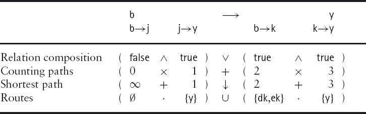
Algebraically there is a commonality among all these problems. Table 16.1 shows how the label of the edge from c to y is computed for four of the problems. (Frequency calculation has been omitted because it is algebraically identical to counting paths. Relation composition is slightly special because the edges are not labelled but it is the existence of an edge that is in question. In algebraic terms, the labels on edges are the booleans.) For relation composition, two connecting edges are combined by conjunction (∧) and a choice of connecting node is effected by disjunction (∨); for counting paths, the labels of two connecting edges are combined by multiplication (×) and a choice of connecting node is effected by addition (+); for shortest paths, the labels of two connecting edges are combined by addition (+) and a choice of connecting node is effected by minimisation (↓); finally, for finding paths, two connecting edges are combined by the product operation defined in (16.31) and a choice of connecting node is effected by set union (∪).

![]() Table 16.1: Computing the label of an edge.
Table 16.1: Computing the label of an edge.
The same process is used when edges are missing. In Table 16.2 we show how the edge labels are combined to determine the label of the edge from b to y in the combined graph. Note that there is no edge from b to j in the left graph. This is modelled by false in the case of relation composition, by 0 in the case of counting paths, by ∞ (infinity) in the case of shortest paths and by ![]() in the case of paths. Recall that
in the case of paths. Recall that false is the “zero” of conjunction, 0 is the “zero” of multiplication, and ∞ is the “zero” of addition. (That is, [ false ∧ x = false ], [ 0×x = 0 ] and [ ∞+x = ∞ ].) It is clear from (16.31) that ![]() is the “zero” of the product of sets of paths.
is the “zero” of the product of sets of paths.
![]() Table 16.2: Combining edge labels.
Table 16.2: Combining edge labels.
The commonality in the algebraic structure is evident when we summarise the rules for combining edges and combining paths in the four cases. This is done in Table 16.3. The first column shows how the labels on two connecting edges are combined. The second column shows how the labels on two paths connecting the same nodes are combined; the name given to the corresponding quantifier is included in brackets. The third column gives the zero of edge combination (i.e. the label given to a non-existing edge) and the fourth column is the formula for determining the (a, c)th element of the relevant product G×H of graphs G and H.
![]() Table 16.3: Rules for combining edges and paths.
Table 16.3: Rules for combining edges and paths.
We recall from Section 12.5.6 that a semiring is a set on which are defined two binary operations + and ×. The set includes two elements 0 and 1; the element 0 is the unit of + and the zero of ×, the element 1 is the unit of ×. In general, if the edges of a bipartite graph G are labelled with the elements of a semiring S, and G has type A∼B, then G is isomorphic to a function of type A×B → S. If bipartite graphs G and H are labelled with the elements of a semiring S, and G has type A∼B and H has type B∼C (for some A, B and C), the (S) product G×H is a bipartite graph of type A∼C; writing a G b for the label given to the edge from a to b (which by definition is the element 0 in S if no edge exists), the labels of the edges of G×H are given by
If G and H both have the same type (i.e. A∼B for some A and B), it makes sense to define G+H. It is a graph of type A∼B; the definition of the edge labels is
Note the overloading of notation in these definitions. On the left side of equality is a new operator which is defined in terms of an existing operator on the right side with exactly the same name (“×” in (16.33) and “+” in (16.34)). This takes some getting used to. Possibly harder to get used to is that the names stand for operators in some arbitrary semiring – in the case of shortest paths, “×” stands for addition (“+”) in normal arithmetic. That can indeed be confusing. The justification for the overloading is the fact that the algebraic properties of the new product and sum operators now look very familiar.
In formal terms, if the edges of a bipartite graph G are labelled with the elements of a semiring S, and G has type A∼B, then G can be identified with a function of type A×B → S. Definitions (16.33) and (16.34) denote application of G to arguments a and b by a G b, and define operators × and + of type
(A×B → S) × (B×C → S) → (A×C → S)
and
(A×B → S) × (A×C → S) → (A×C → S),
respectively. The following theorem records the algebraic properties of these functions.
Theorem 16.35 Graph addition is associative and symmetric. Graph product is associative. Graph product distributes through graph addition. There are graphs 0 and 1 such that 0 is the unit of addition and the zero of product, and 1 is the unit of product.
Formally, suppose S = (S,0,1,+,×) is a semiring. Then, if G and H are functions of type A×B → S, for some A and B, and addition is defined by (16.34), then
[ G+H = H+G ] .
Also, if G, H and K are functions of type A×B → S,
[ (G+H)+K = G+(H+K) ] .
Defining the function 0A∼B of type A×B → S by
![]() a 0A∼B b = 0
a 0A∼B b = 0 ![]() ,
,
we have
[ G+0A∼B = G ] .
If G, H and K are functions of type A×B → S, B×C → S and C×D → S (for some A, B, C and D) and product is defined by (16.33), then
[ (G×H)×K = G×(H×K) ] .
Also, if G is a function of type A×B → S and H and K are functions of type B×C → S (for some A, B and C) then
[ G×(H+K) = G×H + H×K ] .
If G is a function of type B×C → S (for some B and C) and A is an arbitrary set,
[ 0A∼B×G = 0A∼C ] .
Finally, defining the function 1A of type A×A → S by
![]() a 1A a′ =
a 1A a′ = if a = a′ → 1 ![]() a ≠ a′ → 0
a ≠ a′ → 0 fi ![]() ,
,
then, if G is function of type A×B → S (for some A and B),
[ 1A×G = G = G×1B ] .
16.5 MATRICES
Recall that a (bipartite) directed graph is a method of representing a heterogeneous relation of type A∼B . When the types A and B are finite, a relation can also be represented by a boolean matrix. For example, the relation depicted in Figure 16.4 can be represented by the following matrix:

Whereas a bipartite directed graph has a type of the form A∼B, a matrix has a dimension of the form m×n (pronounced “m by n”) for some strictly positive integers m and n. The above matrix has dimension 3×2. Matrices are commonly denoted by bold capital letters, like A and B. It is also common to refer to the rows and columns of a matrix and to index them by numbers from 1 thru m and 1 thru n, respectively. The element of matrix A in row i and column j is often denoted by aij. Sometimes mathematicians write “let ![]() ” as a shorthand for introducing the name of a matrix and a means of denoting its elements. Formally, a matrix of dimension m×n with entries in the set S is a function of type
” as a shorthand for introducing the name of a matrix and a means of denoting its elements. Formally, a matrix of dimension m×n with entries in the set S is a function of type
{i | 1 ≤ i ≤ m} × {i | 1 ≤ i ≤ n} → S.
The matrix representation of finite directed graphs is sometimes exploited in computer software since a matrix corresponds to what is called a two-dimensional array. (In computer software, array indices commonly begin at 0 and not at 1 because this is known to be less error-prone.)
Labelled bipartite graphs can also be represented by matrices of an appropriate type, provided the graph has a finite number of nodes and a suitable representation can be found for non-existent edges.
The graphs in Figure 16.8 were used to illustrate two different problems. In Section 16.4.1, the labels represented a number of different edges and the problem was to count the number of paths from one node to another in the combined graph. In Section 16.4.3, the labels represented distances and the problem was to determine shortest distances. In both cases, the graphs can be represented as a matrix but the representation of non-existent edges is different.
In the case of counting paths, the left-hand labelled graph in Figure 16.8 is represented by the following matrix, where non-existent edges are represented by 0:

In the case of determinining shortest paths, the left-hand labelled graph in Figure 16.8 is represented by the following matrix, where non-existent edges are represented by ∞:

In general, the type of a labelled directed graph has the form A×B → L, where A and B are the two sets of nodes and L is the type of the labels. (This assumes that non-existent edges can be suitably represented by an element of L.) Corresponding to such a graph is a matrix of type
{i | 1≤ i ≤ |A|} × {j | 1 ≤ j≤|B|} → L.
In this way, two-dimensional matrices are graphs except for loss of information about the names of the nodes. Product and addition of matrices is the same as product and addition of graphs.
We conclude this section with an aside. In (engineering) mathematics, matrices are typically assumed to have elements that are real numbers. The standard definition of sum and product of matrices in mathematics corresponds to what we called the “standard” sum and product of graphs in Section 16.4.1. This is how matrix addition and multiplication might be introduced in a conventional mathematics text.
The sum of two m×n matrices A and B is an m×n matrix:
A+B = ![]() aij
aij![]() + bij
+ bij![]() =
= ![]() aij + bij
aij + bij![]()
The product C = AB of the m×n matrix A and the n×r matrix B is an m×r matrix:
![]()
Note that i and j are dummies in an implicit universal quantification. The range of i in both definitions is 1 thru m; the range of j in the definition of A+B is 1 thru n and in the definition of AB is 1 thru r. Note also the overloading of “+” and the invisible product operator.
Matrices are used to formulate the solution of simultaneous equations (in standard arithmetic). The method that children learn is called Gaussian elimination. Gaussian elimination can, in fact, be formulated in terms of path-finding, but this goes beyond the scope of this text.
16.6 CLOSURE OPERATORS
Just as in Section 16.2 we progressed from heterogeneous relations to homogeneous relations, we now progress from labelled bipartite graphs to labelled graphs with a fixed set of nodes, A. As before, the parameter A is sometimes implicit.
The following theorem is just a special case of Theorem 16.35 (albeit a very important special case).
Theorem 16.36 (Graph Semirings) Suppose S = (S, 0, 1, +, ×) is a semiring and suppose A is an arbitrary set. Let 0 and 1 denote, respectively, the functions 0A∼A and 1A defined in Theorem 16.35. Let the addition operator + and the product operator × on elements of A×A → S be as defined in (16.34) and (16.33). Then, with these definitions, (A×A → S, 0, 1, +, ×) is a semiring.
We call (A×A → S, 0, 1, +, ×) the semiring of graphs (with node-set A).
Theorem 16.36 is fundamental to solving many search problems. The problem is modelled as evaluating the paths in a (finite) graph. The semiring S is used to evaluate paths by dictating how to combine the values of edges – their labels–when forming a path (the product operation of S) and how to choose between paths (the sum operation of S). The particular choice of S depends on the nature of the problem to be solved; this could be just showing the existence of a path, finding the length of a shortest path, finding the best path in terms of minimising bottlenecks, and so on.
If G and H are two labelled graphs (with the same node-set), the sum G+H evaluates a choice of edges from G or H. The product G×H evaluates paths of edge-count 2 consisting of an edge in G followed by an edge in H. Similarly, if K is also a graph with the same node-set, (G+H)×K evaluates paths of edge-count 2 consisting of first an edge chosen from the graph G or the graph H and followed by an edge in the graph K.
In this way, the product G×G gives a value to paths of edge-count 2 in the graph G, G×G×G gives a value to paths of edge-count 3. Defining G0 to be 1, G0 gives a value to paths of edge-count 0. In general, Gk evaluates paths in the graph G of edge-count k and ![]() evaluates a choice of all paths in the graph G of edge-count less than n.
evaluates a choice of all paths in the graph G of edge-count less than n.
Care needs to be taken when extending this argument to arbitrary edge-count. For example, if there is a cycle in a graph (a path of edge-count 1 or more from a node to itself), counting the number of paths – as we did in Section 16.4.1 – will increase without limit as n increases. Another example is when distances (see Section 16.4.3) can be negative: if there is a cycle of negative length on a node, the minimum distance between two nodes can decrease without limit as the maximum edge-count of paths is allowed to increase. The infinite summation ![]() is not always meaningful.
is not always meaningful.
Whenever ![]() is meaningful, it is called the reflexive transitive closure of G and denoted by G*. (Note that the semiring giving meaning to the addition and product operations in this expression is a parameter of the definition.) A semiring that admits the introduction of a reflexive transitive closure operator with certain properties is called a regular algebra. (An important example of such a semiring is the semiring of homogeneous relations on a fixed set with addition and product being defined to be set union and relation composition, respectively.) Regular algebra is a fundamental topic in the computing science curriculum, but beyond the scope of this text.
is meaningful, it is called the reflexive transitive closure of G and denoted by G*. (Note that the semiring giving meaning to the addition and product operations in this expression is a parameter of the definition.) A semiring that admits the introduction of a reflexive transitive closure operator with certain properties is called a regular algebra. (An important example of such a semiring is the semiring of homogeneous relations on a fixed set with addition and product being defined to be set union and relation composition, respectively.) Regular algebra is a fundamental topic in the computing science curriculum, but beyond the scope of this text.
16.7 ACYCLIC GRAPHS
A class of graphs for which the summation ![]() is always meaningful is the class of finite, acyclic graphs. Recall that a graph is acyclic if there are no cycles in the graph. This has the obvious consequence that, if the graph has a finite set of nodes, all paths have edge-count less than the number of nodes in the graph – because no node is repeated on a path. That is, G* equals
is always meaningful is the class of finite, acyclic graphs. Recall that a graph is acyclic if there are no cycles in the graph. This has the obvious consequence that, if the graph has a finite set of nodes, all paths have edge-count less than the number of nodes in the graph – because no node is repeated on a path. That is, G* equals ![]() , where n is the number of nodes in the graph.
, where n is the number of nodes in the graph.
One might wonder when acyclicity is relevant. After all, many of the problems discussed in earlier chapters clearly involve undirected graphs, and such graphs always contain cycles!
Of theoretical importance is that the reflexive transitive closure of the relation on nodes defined by an acyclic graph is a partial ordering relation. It is reflexive and transitive by definition. Acyclicity of the graph guarantees that the relation is anti-symmetric.
Acyclicity is relevant to the games discussed in Chapter 4. There we imposed the restriction that all games are guaranteed to terminate, irrespective of how the players choose their moves. In other words, we imposed the restriction that the graph of all moves starting from any initial position has no cycles.
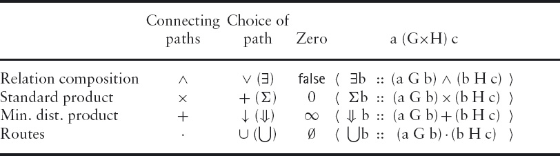
For other problems, it is often interesting to know in how many different ways the problem can be solved. Figure 16.15 shows, on the left, an undirected graph where the problem is to find a path from the start to the finish node.
![]() Figure 16.15: An undirected graph and the subgraph determining paths of minimal edge-count to the finish node.
Figure 16.15: An undirected graph and the subgraph determining paths of minimal edge-count to the finish node.
If we ask the question how many paths there are, the answer is “infinitely many”. A more sensible question is to ask how many paths there are that use a minimal number of edges. This question is answered by the acyclic, directed graph on the right of Figure 16.15. The reflexive transitive closure of this graph gives all the paths from each node to the finish node of minimal edge-count; the graph makes it clear that there are two paths from start to finish that have minimal edge-count. A very simple example of this sort of analysis is the discussion of the goat–cabbage–wolf problem in Section 3.2.1.
Given a graph G with a finite number of nodes and a designated finish node, it is easy to determine a subgraph of G that defines all paths to the finish node of minimal edge-count. Let the distance of a node to the finish node be the edge-count of any path of minimal edge-count from the node to the finish node. The distance of each node to the finish node can be determined by computing in turn the nodes at distance 0, the nodes at distance 1, the nodes at distance 2, etc. The computation starts from the finish node which is the only node at distance 0. The edges of the subgraph are all edges from a node at distance k+1 to a node at distance k, for some k. (The technique of exploring nodes in order of their edge-count distance from the start or finish node is often used in brute-force search.)
16.7.1 Topological Ordering
A common task is to “visit” all the nodes in a finite, acyclic graph collecting some information about the nodes along the way. For example, in a genealogy tree we might want to determine the number of male and/or female descendants of every person recorded in the tree. More formally, suppose that a is a node of the graph, and there are edges e, . . .,f from a to nodes u, . . .,v; suppose also that the nodes u, . . .,v have been assigned values m, . . .,n, and we want to assign to a a value g(e, . . .,f,m, . . .,n) for some function g, which may be different for different nodes. In order to do so, the nodes must be visited in a so-called topological order. In the case of determining the number of male descendants in a genealogy tree, each such function g returns a number. For people with no children the function g (of no arguments) is the constant 0. For each person with children, the function g adds together the number of male children and the number of male descendants of each child. A topological search begins with the people with no children and then ascends the tree level-by-level until the entire tree has been visited.
In general, a topological ordering of the nodes in an acyclic graph is a linear ordering of the nodes that places node a after node b if there is a non-empty path from a to b in the graph. Formally, we are given a relation R on a finite set N such that R* is a partial ordering relation. A topological ordering assigns a number ord.a to each element a in N in such a way that
![]() ∀ a,b : a∈N∧b∈N : a
∀ a,b : a∈N∧b∈N : a R+ b ⇒ ord.a > ord.b ![]() .
.
(Think of R as the relation on nodes defined by the existence of an edge and R+ as the relation corresponding to the existence of paths.)
The following algorithm effects a topological search. The algorithm uses a set V to record the elements of N (the nodes) that have been ordered (“visited”) and a set NV to record the elements of N that have not been ordered (“not visited”). The number k is initially 0 and is incremented each time a node is ordered.
{R* is a partial ordering on the finite set N}
V,NV,k := ![]() ,N,0 ;
,N,0 ;
{Invariant:
V∪NV = N
∧ ![]() ∀ a,b : a∈V ∧ b∈V : a
∀ a,b : a∈V ∧ b∈V : a R+ b ⇒ ord.a > ord.b ![]()
∧ ![]() ∀ b : b∈V : k >
∀ b : b∈V : k > ord.b![]()
∧ ![]() ∀ a,b : a∈V ∧ a
∀ a,b : a∈V ∧ a R b : b∈V ![]()
Measure of progress: |NV| }
do NV = ![]() → choose a∈NV such that
→ choose a∈NV such that ![]() ∀b : a
∀b : a R b : b∈V![]() ;
;
ord., k := k,k+1 ;
remove a from NV and add it to V
od
{V = N ∧ ![]() ∀ a,b : a∈N ∧ b∈N : a
∀ a,b : a∈N ∧ b∈N : a R+ b ⇒ ord.a > ord.b![]() }.
}.
The invariant of the algorithm expresses the fact that, at each stage, the subrelation obtained by restricting the domain of R to V has been linearised,
![]() ∀ a,b : a∈V ∧ b∈V : a
∀ a,b : a∈V ∧ b∈V : a R+ b ⇒ ord.a > ord.b![]()
each element of V having been assigned an order that is less than k,
![]() ∀b : b∈V : k>
∀b : b∈V : k>ord.b![]() .
.
Also, the set of visited nodes V is “closed” under the relation R:
![]() ∀ a,b : a∈V ∧ a
∀ a,b : a∈V ∧ a R b : b∈V![]()
At each iteration, an unvisited node a is chosen such that the only edges from a are to nodes that are already visited:
![]() ∀b : a
∀b : a R b : b∈V![]() .
.
(For nodes with no outgoing edges, the universal quantification is vacuously true; the first iteration will choose such a node.) The precondition that R* is a partial ordering on N is needed to guarantee that such a choice can always be made. If not, the subset NV is not partially ordered by R*. The chosen node is “visited” by assigning it the number k. The sets V and NV and the number k are updated accordingly. The measure of progress gives a guarantee that the algorithm will always terminate: at each iteration the size of the set NV is reduced by 1; the number of iterations is thus bounded by its initial size, which is |N| which is assumed to be finite.
In practice, the linearisation is not the primary purpose and is left implicit. For example, a topological search might be used to count the number of minimal-edge-count paths to a given node. The count begins with the number 1 for the given node (since there is always one path from each node to itself) and then calculates the number of paths for the remaining nodes in topological order, but without explicitly ordering the nodes. If edges of the graph are labelled with distances, topological search is used to determine the shortest path from all nodes to a given node; the search begins at the given node, which is at distance 0 from itself, and then computes the distance of each of the other nodes from the given node in topological order. In this context, the technique is called dynamic programming.
16.8 COMBINATORICS
Combinatorics is about determining the number of “combinations” of things in a way that does not involve counting one by one. For example, if a person has three pairs of shoes, two coats and five hats, we might want to know how many different ways these items of clothing can be combined – without listing all the different possibilities.
16.8.1 Basic Laws
Some basic results of combinatorics were mentioned in Chapter 12: the number of elements in the set A+B (the disjoint sum of A and B) is |A|+|B|, the number of elements in A×B (the cartesian product of A and B) is |A|×|B| and the number of elements in AB (the set of functions from B to A) is |A||B|.
As an example of the use of the first two of these rules, let us point the way to tackling the nervous-couples project (Exercise 3.3). We show how to calculate formally the number of valid states. Refer back to Section 3.3 for the full statement of the problem and the definition of a state.
First we note that a state is completely characterised by the position of the boat and the positions of the presidents and bodyguards. A state is therefore an element of the cartesian product
BoatPosition × PBconfigurations
where BoatPosition is the two-element set {left,right} and PBconfigurations is a set describing the possible configurations of the presidents and bodyguards on the two banks. The number of valid states is therefore
2 × |PBconfigurations|.
(Note that we are counting valid states and not reachable states. For example, a state where the boat is on one bank and all couples are on the other bank is valid, but not reachable.)
The next step is to note that a configuration of the presidents and bodyguards is characterised by the number of presidents and the number of bodyguards on the left bank. (This is because the number of presidents/bodyguards on the left and right banks adds up to N.) Let us use lP and lB to denote these two quantities. Now, a pair (lP, lB) describes a valid configuration exactly when
(Take care: this is the most error-prone step of the analysis because it is the step when we go from the informal to the formal. We have to formulate precisely the constraint that a president may not be on the same bank as a bodyguard unless their own bodyguard is also present. We also have to formulate precisely what it is we are counting. It is often the case that informal problem descriptions are unclear; the purpose of formalisation is to add clarity. Make sure you agree that (16.37) does indeed characterise the valid configurations.)
From (16.37), we conclude that the number of valid president–bodyguard configurations is
In order to simplify this expression, we aim to express the set of president–bodyguard configurations as a disjoint sum. This is done by first rewriting (16.37) as
lB=0 lB=N ∨ 0 < lB = lP < N.
This splits the set of president–bodyguard configurations into three disjoint sets (assuming N≠0), namely the configurations satisfying lB=0, the configurations satisfying lB=N and the configurations satisfying 0 < lB=lP <N. The number of such configurations is, respectively, N+1, N+1 and N−1.
Combining the number of president–bodyguard configurations with the two positions of the boat, we conclude that the number of valid states is
2×((N+1) + (N+1) + (N−1)).
That is, there are 6N+2 valid states. (In the three-couple problem there are thus 20 valid states and in the five-couple problem there are 32 valid states.)
16.8.2 Counting Choices
A typical problem that is not covered by the laws for disjoint sum, cartesian product and function spaces is in how many ways m indistinguishable balls can be coloured using n different colours. Although the problem involves defining a function from balls to colours, it is complicated by the fact that balls are indistinguishable.
Fundamental to such problems is the notion of a “permutation” of a set. A permutation of a set A is a total ordering of the elements of A. If A is finite, a permutation of A is specified by saying which element is first, which element is second, which is third, and so on to the last. If A has n elements, there are n ways of choosing the first element. This then leaves n−1 elements from which to choose the second element. Thus there are n×(n−1) ways of choosing the first and second elements. Then there are n−2 elements from which to choose the third element, giving n×(n−1)×(n−2) ways of choosing the first, second and third elements. And so it goes on until there is just one way of choosing the nth element. We conclude that there are ![]() different permutations of a set of size n. This number is called n “factorial” and denoted by n!. Although the notation is not standard, by analogy with the notations for disjoint sum and cartesian product, we use the notation A! for the set of permutations of A. This allows us to formulate the rule
different permutations of a set of size n. This number is called n “factorial” and denoted by n!. Although the notation is not standard, by analogy with the notations for disjoint sum and cartesian product, we use the notation A! for the set of permutations of A. This allows us to formulate the rule
[ |A!| = |A|! ] .
Note that the empty set has 0 elements and ![]() equals 1. So
equals 1. So
|![]() !| = 0! = 1.
!| = 0! = 1.
In general there are
![]()
ways of choosing in order m elements from a set of n elements. This formula is sometimes denoted by P(n,m). Noting that (n−m)! is ![]() , it is easy to derive the following definition of P(n,m):
, it is easy to derive the following definition of P(n,m):
Now we turn to the problem of determining in how many ways it is possible to choose a subset with m elements from a set of n elements, which we denote (temporarily) by C(n,m). So, for example, if there are six differently coloured balls, in how many ways can we choose four of them? That is, what is the value of C(6,4)?
The solution is to consider an algorithm to choose in order m elements from a set of n elements. The algorithm has two phases. First we choose a subset with m elements from the set of n elements. This can be done in C(n,m) ways. Next we choose a particular ordering of the m elements in the chosen subset. This can be done in m! ways. Combining the two phases, there are
C(n,m) × m!
ways of choosing in order m elements from a set of n elements. But this is what we denoted above by P(n,m). That is,
[ P(n,m) = C(n,m) × m! ] .
With some simple arithmetic combined with (16.39), we conclude that
We said above that we would use the notation C(n,m) only temporarily. The reason is that the quantity is considered so important that it deserves a special notation. The notation that is used is ![]() and it is called a binomial coefficient.3 The definition (16.40) thus becomes:
and it is called a binomial coefficient.3 The definition (16.40) thus becomes:
As an example, the number of ways of choosing 4 colours from 6 is ![]() which equals
which equals ![]() This simplifies to
This simplifies to ![]() (i.e. 15). Note that
(i.e. 15). Note that
![]()
The number of ways of choosing a subset of size m is the same as the number of ways of choosing a subset of size n−m. In particular, the number of ways of choosing a subset of size 0 is 1, which is the same as the number of ways of choosing a subset of size n. (A subset of size n is the whole set.) The formula (16.41) remains valid when m equals n or m equals 0 because 0! is defined to be 1. Another special case is that of choosing 1 element from a set of n elements. Formula (16.41) predicts that ![]() is n, as expected.
is n, as expected.
16.8.3 Counting Paths
Many combinatorial problems are solved by so-called recurrence relations and, as we have seen in this chapter, relations can be represented by graphs. Combinatorial problems are thus often solved by a process that is equivalent to counting paths in a graph. Some problems have a lot of structure – they involve “recurring” patterns, which enables their solution to be formulated as compact mathematical formulae. Many problems, however, have only limited structural properties. They can still be solved by counting paths in a graph, but their solution cannot be given in the form of a compact mathematical formula; instead their solution involves the use of an efficient algorithm. This section is about two examples, one much more structured than the other.
Recall the ball-colouring problem mentioned above: in how many ways can m indistinguishable balls be coloured using n colours. Suppose the colours are given numbers 1, 2, . . ., n. A colouring of the balls defines a function no. such that no.c is the number of balls with colour c. (So no.1 is the number of balls with colour 1, no.2 is the number of balls with colour 2, and so on.) All balls have to be coloured, so it is required that
no.1+no.2+ . . . +no.m = n.
![]()
The “coefficient“ of xm×yn−m is thus ![]() .
.
The problem is to determine the number of functions no. that have this property. In words, it is the number of different ways of partitioning the number n into m numbers.
One way to solve the problem is to imagine an algorithm to perform the partitioning. Suppose we place all the balls in a line, which we represent by a sequence of bs. For example, if there are seven balls we begin with the sequence
b b b b b b b.
Now suppose there are three colours. We choose how to colour the balls by inserting vertical lines, representing a partitioning of the balls. For example, the sequence
b | b b | b b b b
assigns one ball the first colour, two balls the second colour and four balls the third colour. The sequence
| b b b b b b b |
assigns all balls the second colour and none the first or third colour.
If there are m balls and n colours, the sequence has length m+n−1. It is formed by choosing m positions to place a b, the remaining positions then being filled with the partitioning symbol “|”. In this way, we conclude that the total number of colourings is
![]()
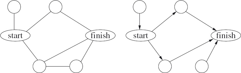
A way of visualising the above algorithm is by means of a graph. Figure 16.16 shows the graph for the case where there are five balls and three colours. The arrangement of the balls in a line is shown by the numbers above the graph and the colours are shown by the numbers at the side of the graph. The nodes in the graph are the points where two lines meet. Starting from the top-left corner and traversing a path to the bottom-right corner represents the process of constructing a sequence of bs and partition symbols, symbol by symbol. Horizontal moves correspond to adding a b to the sequence, and vertical moves to adding a partition symbol. At the top-left corner, the position labelled (5, 3), nothing has been done; at the bottom-right corner, the position labelled, (0, 1), the balls have been completely partitioned. At an intermediate node, a position labelled (i, j), the balls to the left of the node have been assigned colours and those to the right have not; i is the number of balls remaining to be coloured and j is the number of colours that are to be used. Choosing to move horizontally from position (i, j) to position (i−1, j) represents adding a b to the sequence, that is, choosing to colour another ball with colour j. Choosing to move vertically from position (i, j) to position (i, j−1) represents choosing not to give any more balls the colour j. The number of colourings is the number of paths from the top-left node to the bottom-right node.
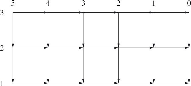
![]() Figure 16.16: Counting ball colourings.
Figure 16.16: Counting ball colourings.
The number of paths from the top-left to the bottom-right node in an (m+1)×(n+1) acyclic, rectangular grid is ![]() (or equally
(or equally ![]() ). This is because each path has edge-count m+n of which m are horizontal edges and n are vertical edges.
). This is because each path has edge-count m+n of which m are horizontal edges and n are vertical edges.
Now, from the top-left node of such a graph, each path begins with either a horizontal edge or a vertical edge. This divides the paths into a disjoint sum of paths. Moreover, a path that begins with a horizontal edge is followed by a path from the top-left to the bottom-right node in an ((m−1)+1)×(n+1) rectangular grid; similarly, a path that begins with a vertical edge is followed by a path from the top-left to the bottom-right node in an (m+1)×((n−1)+1) rectangular grid. We thus conclude that
Property (16.42) is an example of what is called a recurrence relation. It is a relation between binomial coefficients defined by an equation in which the coefficients “recur” on both the left and right sides. This particular property is called the addition formula for binomial coefficients.
The graph in Figure 16.16 has a very regular rectangular-grid structure. Other combinatorial problems are not so well structured but can still be expressed as counting the number of paths in an acyclic graph. For such problems the use of topological search (or a similar algorithm) to compute the number of paths is unavoidable. Let us illustrate this by returning, for the last time, to the nervous-couples problem first introduced in Section 3.1.
Figure 16.17 shows the state-transition diagram for getting three couples across the river. Of the 20 valid states, it shows just the 16 that can be reached from the starting position of three couples on the left bank. (Four states not shown are valid, but no move is possible to or from each of them.) The notation introduced in Section 3.3.3 is used for indicating the positions of the presidents and their bodyguards; this is supplemented by a short horizontal line to indicate the position of the boat.
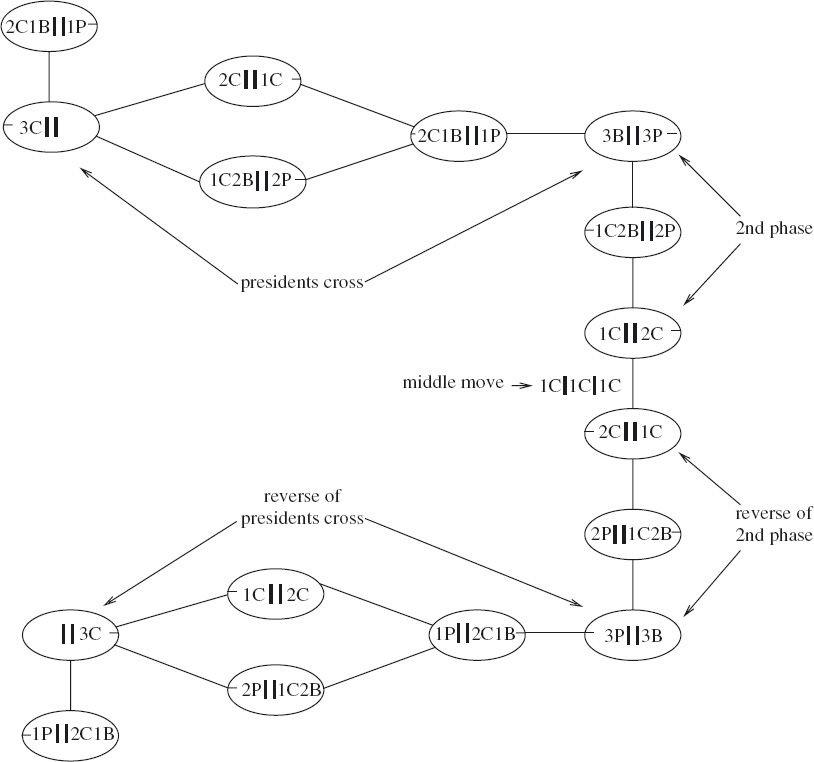
![]() Figure 16.17: Three nervous couples: state-transition diagram.
Figure 16.17: Three nervous couples: state-transition diagram.
The structure of Figure 16.17 reflects the decomposition of the problem discussed in Section 3.3.4. The set of solutions is symmetric about a middle move in which one couple crosses from right to left. Preparatory to this middle move, the presidents first cross and then two additional moves are needed to get to a position where the middle move can be executed. These two additional moves are called the “2nd phase” in Figure 16.17. Following the middle move, the presidents’ and 2nd-phase moves are reversed.
It is clear from Figure 16.17 that, if the individual presidents and/or bodyguards are not distinguished, there are just four different ways of getting everyone across with the minimum number of crossings. However, let us suppose we distinguish them all by giving each person a name. How many different ways of getting them across are there now?
It is not necessary and, indeed, it is impractical to redraw the state diagram. It suffices to label each edge with a number that gives the number of different crossings of each type. (Refer back to Section 16.4.1 for further explanation.) In addition we exploit the symmetric structure of the graph.
Figure 16.18 shows three of the five component parts of the state diagram relevant to getting the couples across the river in a minimum number of crossings: getting the presidents across the river, the 2nd phase and the middle crossing. (Symmetry allows us to omit the remaining two component parts.) Arrowheads have been added to show the direction in which the state change occurs. More importantly, the label on each edge gives the number of crossings of that type. For example, there is a label of 3 on the edge from the state 3C || to the state 1C,2B || 2P because there are (![]() ) ways (i.e. 3 ways) of choosing 2 (named) presidents to cross the river. Similarly, the middle crossing has the label 2 because there are 2 ways of choosing a couple from 2 couples to make the crossing.
) ways (i.e. 3 ways) of choosing 2 (named) presidents to cross the river. Similarly, the middle crossing has the label 2 because there are 2 ways of choosing a couple from 2 couples to make the crossing.
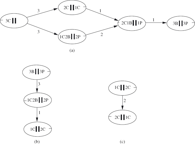
![]() Figure 16.18: Counting crossings: (a) presidents cross; (b) 2nd phase; (c) middle crossing.
Figure 16.18: Counting crossings: (a) presidents cross; (b) 2nd phase; (c) middle crossing.
We can now use a simple topological search to evaluate the number of paths from start to finish in each of the component graphs. In the 2nd phase, there are 3×1 (i.e. 3) different paths and there are (3×2 + 3×1)×1 (i.e. 9) paths that get the presidents across. The final step is to combine all the components. The number of ways of getting all the couples across the river when each individual is named is
9×3×2×3×9.
That is, there are an astonishing 1458 ways of getting them across!
This example is very suitable for concluding this text because it illustrates a potential pitfall of poor problem-solving technique, namely an unnecessary explosion in the size of the space in which solutions are sought. A crucial first step in algorithmic problem solving is to clearly identify what is relevant and what is not relevant. This is reflected in how the problem is represented formally. Choosing the wrong representation can turn a relatively simple problem into one that is impossible to solve in practice. Even in the cases where a simple problem remains tractable, solutions should be carefully reviewed in order to eliminate unnecessary complexity.
16.9 EXERCISES
1. Draw the graphs corresponding to the following relations. Assume that each has type {a,b,c,d} × {u,v,w}.
(a) {(a, u), (b, v), (c, w)}
(b) {(a, u), (a, v), (a, w), (b, v), (c, w)}
(c) The universal relation.
(d) The empty relation.
2. Figure 16.19 depicts a homogeneous relation. Let us call the relation R. Construct the first four powers of R (i.e. R0, R1, R2, R3).
Suppose you are asked to calculate ![]() for successive values of n (starting from n = 0). At some stage, the value does not change. That is, for some value of n,
for successive values of n (starting from n = 0). At some stage, the value does not change. That is, for some value of n,
![]()
By inspecting the graph, can you determine the smallest number n for which this is the case without actually calculating the value of ![]() ?
?
3. Suppose the rightmost node in the graph shown in Figure 16.19 is called the finish node. Construct a graph that depicts all minimal-edge-count paths from nodes in the graph to the finish node. Do so by identifying which nodes are at (edge-count) distance 0, 1, 2, etc. from the finish node and including those edges in the given graph that are from a node at distance k+1 to a node at distance k for some k.
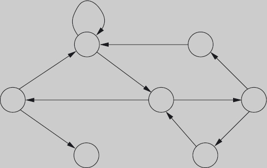
![]() Figure 16.19: A homogeneous relation.
Figure 16.19: A homogeneous relation.
4. A labelled acyclic graph is depicted in Figure 16.20. In the graph, one node has no incoming edges and one node has no outgoing edges. Call these the start and finish nodes, respectively.
(a) Suppose the edge labels count the number of edges between a pair of nodes. Use topological search to determine how many different paths there are from the start to the finish node.
(b) Suppose the edge labels represent distances. Use topological search to determine the length of a shortest path from the start to the finish node.

![]() Figure 16.20: An acyclic graph.
Figure 16.20: An acyclic graph.
5. Consider the graph in Figure 16.20 again. Suppose the edges now represent low bridges, the edge label being the height of the bridge. It is required to drive a load from the start node to the finish node that maximises the height of the lowest bridge on the path. Identify the appropriate product and sum operations on paths and calculate the best path according to this criterion.
6. Consider the graph in Figure 16.20 yet again. Suppose the edges of the graph represent tasks. A node connecting two edges means that one task must be completed before the next task can be begun. (For example, when building a house a task might be to lay the foundations. This task must be completed before the walls can be built.) The label on an edge represents the estimated time to complete the task.
Suppose the problem is to determine the shortest time to complete all tasks from start to finish, assuming that as many tasks as possible are done simultaneously. For the graph shown in Figure 16.20, calculate the shortest time.
Hint: formulate the problem as a path-finding problem. Formulate how two connecting paths should be combined (the product operation) and how a choice is made between two paths between the same pair of nodes.
(In operations research, a graph that represents orderings between tasks and the time to complete each task is called a Gantt chart.)
7. The topological search algorithm in Section 16.7.1 assumes that R* is a partial ordering. How would you modify the algorithm so that it tests whether or not R* is a partial ordering?
1Beware: for some problems it is better to convert a self-loop into two copies of the same directed edge.
2We have not forgotten 0. The definition of R0 is introduced later when we consider the reflexive transitive closure of a relation. It does indeed correspond to paths of length 0.
3The name comes from the expansion of the “binomial” (x+y)n as a sum of products: