
Chapter 1
Early Diagnosis of Neurodegenerative Diseases from Gait Discrimination to Neural Synchronization
Shamaila Iram1, Francois-Benoit Vialatte2, and Muhammad Irfan Qamar3 1University of Salford, Greater Manchester, UK 2Laboratoire SIGMA, ESPCI ParisTech, Paris, France 3IBM Canada Ltd., Canada
E-mail: [email protected], [email protected], [email protected]
E-mail: [email protected], [email protected], [email protected]
Abstract
It is generally believed that early detection of neurodegenerative diseases will provide a much more sustainable framework for dealing with age-related diseases in the future. This chapter presents a strategic framework for the early diagnosis of neurodegenerative disease from gait discrimination to neural synchronization. Here, we propose and present a new classifier fusion strategy that combines classification algorithms and rules (voting, product, mean, median, maximum, and minimum) to measure specific behaviors in people with neurodegenerative diseases. On the other hand, it is now evident that electroencephalographic (EEG) signals of patients with Alzheimer disease usually have less synchronization than those of healthy subjects. Computing neural synchronization of EEG signals to detect any perturbation will help diagnose this fatal disease at an earlier stage. Three neural synchrony measurement techniques, phase synchrony, magnitude-squared coherence, and cross-correlation, are applied to analyze three different databases of mild Alzheimer disease patients and healthy subjects to compare the right and left temporal lobe of the brain with the rest of the brain area. Results are compared using Mann–Whitney U statistical test.
Keywords
Combining Classifiers; Pattern Recognition; Machine Learning; Behavior classification; Neurodegenerative Diseases; Movement Signals; Electroencephalographic Signals; Neural Synchronization; Cross-correlation; Phase synchrony; Coherence; Mann–Whitney U TestIntroduction
Advancements in machine learning provoke new challenges by integrating data mining with biomedical sciences in the area of computer science. This emergent research line provides a multidisciplinary approach to combine engineering, mathematical analysis, computational simulation, and neuro-computing to solve complex problems in medical science. One of the most significant applications of machine learning is data mining. Data mining provides a solution to find out the relationships between multiple features, ultimately improving the efficiency of systems and designs of the machines. Data-mining techniques provide computer-based information systems to find out data patterns, generate information for the hidden relationships, and discover knowledge that unveils significant findings that are not accessible by traditional computer-based systems.
Neurodegenerative diseases (NDDs) are accompanied by the deterioration of functional neurons in the central nervous system. These include Parkinson, Alzheimer, Huntington, and amyotrophic lateral sclerosis (ALS) among others. The progression of these diseases can be divided into three distinct stages: retrogenesis, cognitive impairment, and gait impairment. Retrogenesis is the initial stage of any NDD which starts with the malfunctioning of the cholinergic system of the basal forebrain that further extends to the entorhinal cortex and hippocampus [1]. During retrogenesis, the patient’s memory is severely affected as a result of the accumulation of pathologic neurofibrillary plaques and tangles in the entorhinal cortex, hippocampus, caudate, and substantia nigra [2]. This stage is known as cognitive impairment. Finally, a patient cannot maintain his or her healthy, normal gait because of disturbances in the corticocortical and corticosubcortical connections in the brain, for example, frontal connection with parietal lobes and frontal lobes with the basal ganglia, respectively [3].
Early detection or diagnosis of life-threatening and irreversible diseases such as NDDs (Alzheimer, Parkinson, Huntington, and ALS) is an area of great interest for researchers from different academic backgrounds. Diagnosing NDDs at an earlier stage is hard, where symptoms are often dismissed as the normal consequences of aging. Moreover, the situation becomes more challenging where the symptoms or data patterns of different NDDs turn out to be similar, and discrimination among these diseases becomes as crucial as the treatment itself. In this chapter, we claim the significance of analyzing gait signals for discriminating movement disorders in different NDDs for accurate diagnosis and timely treatment of patients as well as an early diagnosis of these diseases using EEG signals.
One significant tool for the discrimination of different NDDs is gait signals. Hausdorff et al. [4] suggested that understanding the relationship between loss of motor neurons and perturbation in the stability of stride-to-stride dynamics can help us to monitor NDD progression and in assessing potential therapeutic interventions. Furthermore, they claimed a reduced stride-interval correlation with aging in Huntington disease. Later in 2010, the same gait signals were used by Yunfeng and Krishnan [5] to estimate the probability density functions (PDFs) of stride intervals and its two subphases for Parkinson disease. Moreover, Masood et al. used the same data set of gait signals for the discrimination of different NDDs [6].
The other important tool for early diagnosis and treatment of neurological and neurodegenerative diseases is the electroencephalographic (EEG) signals. Hans Berger was the first to measure EEG signals in humans, and even today the EEG is extensively used to evaluate neurological diseases [7]. The EEG signals originate from the cerebral cortex and evoked by auditory and somatosensory stimuli.
The goal here is to implement a data-mining approach with innovative ideas, using gait and EEG signals as a discriminative and diagnostic tool, to design a diagnostic and therapeutic system for early diagnosis of life-threatening diseases such as Alzheimer, Parkinson, Huntington, and ALS.
Research Challenges
This section provides a detailed insight into the challenges and the problems that need to be looked into, from two different perspectives—challenges with the early diagnosis of NDDs and issues related to machine learning.
Issues with the Early Diagnosis of NDDs
NDDs, especially Alzheimer disease (AD), are the most prevalent form of dementia, and according to statistics, 5%–10% of the population above the age of 65 years are affected by these diseases [8]. The clinical symptoms of the disease are characterized by progressive amnesia, linking it with the continuous and gradual loss of cognitive power and, finally, paralyzing the person by affecting the motor neurons. NDDs triggered by the deterioration of neuronal cells due to accumulation of neurofibrillary tangles and pathological proteins (such as α-synuclein, tau proteins, etc.) and also the senile plaques in corticocortical and corticosubcortical parts of the brain [2]. Because the occurrence of memory loss can be related to one of the aging factors, the ability to predict or diagnose a NDD turns out to be impossible at an earlier stage.
The loss of cognitive power is generally associated with a decrease of functional synchronization of different parts of the brain. Hence, loss of functional interaction between cortical areas could be considered a possible symptom of any NDD. Finding the synchronization in terms of coherence and correlation can possibly provide significant information in the early diagnosis of NDDs. However, the compactness of EEG signals due to various frequency bands makes this task less straightforward. Still more research is required to find out the exact role of each frequency band in the early diagnosis of these diseases.
Issues Related to the Machine Learning Approach
In the context of machine learning, data mining offers many challenges that need to be considered to get optimal results from a classifier. These factors can affect the mining process in terms of computation time, extraction and selection of appropriate features, and implementation of new approaches that can help us get the expected results. This section briefly states those challenges:
• Skewed data sets: Learning of a classifier from an imbalanced data set usually generates biased results. In this case, a classifier becomes more sensitive (highly trained) for the majority class and less sensitive (less trained) for the minority class. Ultimately, the results obtained from such classification make the situation more complicated, especially when the data are being processed from a real-time environment—biomedical, genetics, radar signals, intrusion detection, risk management, and credit card scoring [9].
• Handling missing data: There are many reasons behind missing entries in a data set. A damage in the remote sensor network, failure of gene microarray to yield gene expression, fingerprints, dust or manufacturing defects, and missing applicable tests while diagnosing patients, for example, can lead to missing entries in a data set, as described by Marlin [10]. Feature extraction and classification based on such data sets can lead to unreliable results. Problems of missing data should be investigated before starting a computation process.
• Multiclass data sets: The problem of skewed data sets becomes even more complicated when it comes to multiclass data sets. Practically speaking, in real-world environments, mostly the data sets come from a multiclass domain, for instance, protein fold classification [11]. These multiclass data sets pose new challenges as compared to simple two-class problems. Zhou et al. [12] argue that handling multiclass data sets is much harder than handling two-class problem domains. Jeopardizing the problem further, almost all classifier evaluation techniques are designed for two-class problems and happen to be unfit for multiclass problems.
• Extraction and selection of relevant features: The accuracy of a classifier is directly dependent on the variables that are provided for the classification. The analysis of gait as well as EEG signals and extraction of relevant information is not an easy task. Gait signals may be contaminated with other muscle movement signals or by the environmental data. Similarly, EEG signals may contain the signals of eye movements or externally generated signals (power line, electrode movement, etc.). In the presence of these artifacts, discrimination or classification leads to wrong results. This problem calls for preprocessing steps to get clean signals before classification. Once the signals are extracted, the next challenge is the selection of the most relevant features among others. This not only saves computation time but also reduces the complexity of the system.
• Data Filtering: Previous studies focus on the analysis of compact EEG signals without filtering them into narrow frequency bands. However, this lack of filtration does not provide optimal information about the frequency band, which is more important for detecting Alzheimer (or other NDDs) at its earlier stage.
• Selection of a Classifier: In the field of pattern recognition, the main focus is the successful classification of the features with the maximum possible accuracy rate. A classifier with a specific set of features may or may not be an appropriate option for another set of features. Moreover, different classification algorithms achieve varying degrees of success in different kinds of applications [13]. For this reason, selection of an appropriate classifier becomes a challenging task. Indeed, further research is needed to generalize the performance of the classifiers.
Neurodegenerative Diseases
Neurodegenerative disease is an umbrella term used to describe medical conditions that directly affect the neurons within the brain [14]. These include Parkinson, Alzheimer, Huntington, and ALS. Patients with these kinds of disease experience cognitive decline over a long period, and symptoms include gait abnormalities, problems with speech, and memory loss due to progressive cognitive deterioration [15].
Alzheimer Disease
The changes in the brain that accompany these symptoms are the “tangles” and “plaque” of a toxic protein—amyloid beta (Aβ). These pathological neurofibrillary tangles accumulate in the entorhinal cortex and the hippocampus in the brain, areas that are responsible for the short- and long-term memory of a person [16]. Neuroscientists have reported that in order to keep memory alive, the communication between these two parts is very essential, and any hurdle between these two regions breaks the circuit and leads toward memory disturbance and eventually memory loss [2].
Parkinson Disease
Parkinson disease is characterized by the dopaminergic deterioration process of the nerve cells of substantia nigra [17], a part of the brain responsible for the production of “dopamine”—a chemical that works as a neurotransmitter for controlling movements in different parts of the body. The degenerative process starts from the base of the brain, leading to the destruction of olfactory bulbs, followed by the lower brain stem and subsequently substantia nigra and midbrain [18]. Eventually, it destroys the limbic system and frontal neocortex, resulting in cognitive and psychiatric symptoms.
Huntington Disease
A specific part of the brain, PolyQ, has the Huntington gene with 11–34 repeated sections of glutamine—responsible for the production of cytoplasmic protein called Huntington. When the PolyQ region generates more sections of glutamine, a mutant Huntington protein is produced, which is the actual cause of Huntington disease [19]. This disease is an incurable hyperkinetic motor disorder. The primary symptoms of this disease are jerky and shaky movements, called chorea [20].
Amyotrophic Lateral Sclerosis
To date, it is believed that the actual cause of this disease is a mutant gene, superoxide dismutase 1 (SOD1), that affects the motor neurons of the brains. Moreover, toxicity in cerebrospinal fluid (CSF) is also considered a cause of neuron degeneration [21]. Motor neurons are the nerve cells that are responsible for voluntary movement of the muscles [22]. Weakness in arms and leg muscles is the initial symptom of ALS, which is followed by severe attacks to chest muscles, leaving patients unable to breathe [23].
Classification Algorithms for NDDs
Several methods have been proposed and used for detection of NDDs. Most approaches focus on cognitive decline, biomarkers, and direct analysis of metabolites or genes [24]. However, in recent years, early detection and neuroimaging techniques [25], including genetic analysis, have been commonly used to detect potentially life-threatening diseases like cancer, cystic fibrosis, and neurologic diseases. Mini-Mental State Examination (MMSE) and symptom quantification are other well-known techniques commonly used to diagnose NDDs. Nonetheless, the use of computer algorithms and visualization techniques are considered fundamental to support the early detection process.
Although these approaches provide obvious benefits, current applications for classifying medical data still lack consistency in terms of revealing hidden significant information, especially from real-time clinical data. The main limitation with the approaches is that they only consider a small number of classifiers. Furthermore, many of them fail to include relevant and important features, such as age and gender, that can have a significant impact on results. Moreover, overall accuracy depends on a single set of variables, although other variables potentially could have greater impact on performance evaluation [26]. The approach posited here considers all well-established classification algorithms and uses a large-scale feature set. Each variable in the array has its own significant relationship with the progression of specific diseases. Moreover, rather than relying on base-level classifiers, a new strategy is described based on the fusion of classifiers. In this way, it will be possible to explore any new dimensions that may emerge from the results.
Classifier Fusion Strategy
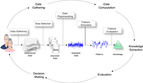
The classifier fusion strategy incorporates several distinct processes—data gathering, feature extraction, and feature evaluation—as illustrated in Figure 1.1. Combining these processes provides a system for processing gait data to support the early detection of specific NDDs. Industry-led data sets with toolsets designed for processing large biomedical data are used to provide a solution for the early detection of NDDs that performs better than several well-known approaches. Using this unique configuration, new toolsets are provided for real-time symptomatic data analysis of NDDs to support diagnostic and treatment strategies.
Data Gathering and Data Preprocessing
In this study, gait data for healthy subjects and patients with Huntington, Parkinson, and ALS, extracted from Physionet1 data sets, are used. The data sets contain data for 16 healthy control subjects (14 females, 2 males), 15 Huntington patients (9 females, 6 males), 15 Parkinson patients (5 females, 10 males), and 13 patients with ALS (3 females, 10 males). Patients with NDDs all have movement problems and are at the final stages of the disease.
As a preprocessing step, relevant features are extracted from integrated data. After completing this stage, all extracted features are meaningful and ready for classification. In this study, 3000 “motion vector” values for left and right foot strides of each subject were extracted over a 10-second period. The mean values obtained from the motion vectors are used to eliminate erroneously recorded data.
Imbalanced Data Sets and Resampling of Data
Learning from imbalanced data sets is an important and controversial topic, which is addressed in our research. These kinds of data sets usually generate biased results [27]. For instance, imagine a medical data set with 50 true negative values (majority class) and 20 true positive values (minority class). If half is selected for training and the remainder for testing (25 healthy and 10 sick persons), we find that the accuracy is 90%. The result suggests that the classifier performs reasonably well. However, what happens is that when all the negative values are accurately identified (healthy persons) and only 5 of the 10 positive values (sick persons) are classified correctly. In this situation, the classifier is more sensitive to detecting the majority class patterns but less sensitive to detecting the minority class patterns. This is because the training data are imbalanced. In other words, the classifier concludes that 5 of the 10 unhealthy people are healthy when this is not the case. These kinds of results ultimately cause more destruction if the data come from real-time environments, such as biomedicine, genetics, radar signals, intrusion detection, risk management, and credit card scoring [9].
In order to solve the imbalanced data set problem, it is necessary to resample data sets. Different resampling techniques are available to achieve this, including undersampling and oversampling [28]. Undersampling is a technique wherein we reduce the number of patterns within the majority class data set to make it equivalent to other classes. In oversampling, more data are generated within the minority class. In this study, as a result of a short number of data sets for each class consequently, oversampling is adopted.
There are eight features in each class, which include signals for the right foot, signals for the left foot, age, height, weight, body mass index, time, and walking speed. For each variable, the minimum and maximum values are calculated. Then, random pseudo-numbers between these values are generated to produce 20 equal patterns for each class.
Feature Classification
The data set containing the eight features described in the previous section provides the feature sets required to diagnose NDDs accurately. More specifically, this data set is used to select a classifier, train it, test it, and finally evaluate the result to determine if the correct classification is performed.
The computation is directly proportional to the number of features considered in the data set. Figure 1.2 demonstrates a scatter plot using only three selected features and shows the complexity of classification of gait patterns for each subject. In this instance, Features 1 and 2 are associated with right and left foot movement signals, whereas Feature 3 represents age, which is considered an important factor in disease progression.
Using the defined feature set, several classifiers have been evaluated for consideration in the final classifier fusion strategy. The principal goal is to use classifiers that perform the best. The classifiers considered are the linear discriminant classifier (ldc), quadratic discriminant classifier (qdc), and the quadratic Bayes normal classifier (udc) for density-based classification. For linear classification, an additional four classifiers are selected, which are the logistic linear (loglc), Fisher’s (fisherc), nearest means (nmc), and the polynomial (polyc). A linear classifier predicts the class labels based on a weighted linear combination of features or the predefined variables. The Parzen (parzenc), decision tree (treec), support vector machine (svc), and k-nearest neighbor (knnc) classifiers have been selected for nonlinear classification of our data sets. The results produced by all 11 classifiers are illustrated in Figure 1.3.
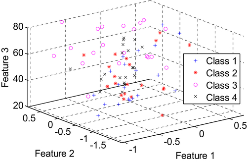
Figure 1.2 Dimensional Scatter Plot of Selected Features where Class 1, Class 2, Class 3, and Class 4 represent “healthy”, “Huntington”, “Parkinson” and “ALS”, respectively.
The results illustrated in Figure 1.3 were evaluated using a confusion matrix table to determine the performance of each classifier. In this instance, the confusion matrix technique was used to determine the distribution of errors across all classes. The estimate of the classifier is calculated as the trace of the matrix divided by the total number of entries. Additional information that a confusion matrix provides is the point where misclassification occurs. This shows the true-positive, false-positive, true-negative, and false-negative values. Diagonal elements show the performance of the classifier, whereas off-diagonal elements represent the errors.
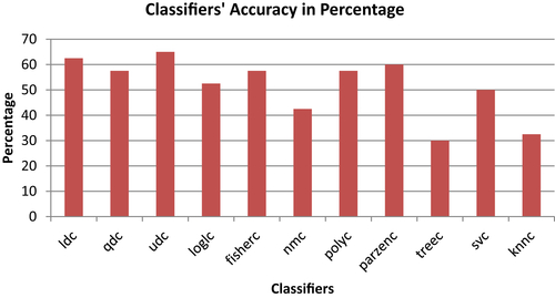
Building on the previous set of results described previously, this section considers the three best-performing classifiers for inclusion in the fusion classifier strategy. From the 11 classifiers, tested the linear discriminant classifier (ldc), the quadratic Bayes normal classifier (udc), and the Parzen Classifier (parzenc) provide the best results with accuracies of 62.5%, 65%, and 60%, respectively. These base classifiers were selected and included in the fusion strategy. Figure 1.4 demonstrates the classifiers fusion strategy, in general.
Figure 1.5 describes the scenario and illustrates the simulated results obtained during the evaluation of gait signals using the 11 base-level classifiers. The results obtained from the three best-performing classifiers are stored in a single array, and their error rates are computed. The mean error rate for the three classifiers is 0.42. The same three classifiers are then combined into a cell array using six different rules. The mean error rate for the combined classifiers is 0.40, which is slightly less than the mean of the base-level classifiers.
The base classifier evaluation and fusion classifier strategy was implemented using Matlab. The base-level classifiers are combined into a cell array using a set of fixed combining rules. Six different rules were analyzed: minimum selection (minc), maximum selection (maxc), median selection (medianc), mean selection (meanc), product combiner (prodc), and voting selection (votec). The evaluation of a cell array of trained classifiers (v and vc) is done by testing the (testset) set.
Evaluation
This section presents the results for experiments performed on the fusion classifier strategy. In this study, the multiclass receiver operating characteristic (ROC) analysis technique is used. This technique is useful for analyzing several different classes, in our case four different classes. First, the classifiers are evaluated in Matlab using the testc routine, which provides several performance estimates for a trained classifier on a test data set. The mean value produced by the test results for individual classifiers is 0.42, which is an error rate. In comparison, the mean value for combined classifiers is 0.40, which is obtained by combining different classification rules. This has clearly shown that the combined classification technique works better than the individual use of classifiers. Moreover, the results depict that the voting combination rule works more efficiently than other combining rules used. Using the voting combination rule, the prediction of the base-level classifiers is combined according to a static voting scheme, which does not change when changes are made to the training set.
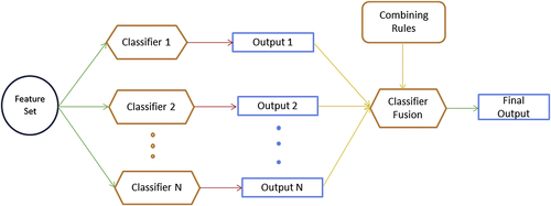
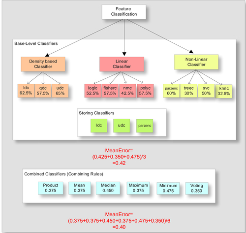
Figure 1.6 shows the results of the ROC analysis for the base-level classifiers, where the quadratic Bayes normal classifier shows the least error rate compared to all other classifiers. In this case, Error I represents the false-positive values, whereas Error II presents the false-negative values that show the system’s failure to predict any disease and label the objects as healthy persons. As can be noted from Figure 1.6, the uncorrelated quadratic Bayes normal classifier generated fewer errors and produced better classification when benchmarked with the Bayes normal-1 and Parzen classifiers. This is because quadratic Bayes normal classifier (Bayes normal-U) uses uncorrelated variables.
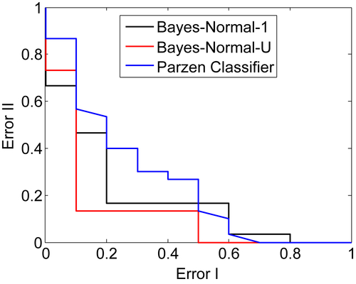
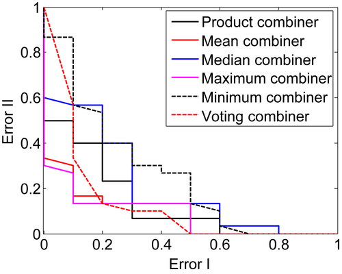
Figure 1.7 shows the results when classifiers are combined using various combining rule algorithms that include the product, the mean, the median, the maximum, the minimum, and the voting combining rules. As shown in Figure 1.7, the best result that produces the least error is the “voting combiner” with a value of 35.0%. This is closely followed by the “product combiner,” “mean combiner,” and “maximum combiner,” with other rules such as “median combiner” and “minimum combiner” showing 45.0% and 47.5% errors, respectively.
Neural Synchronization and Data Collection
Synchronization, precisely speaking, is a coordination of “rhythmic oscillators” for a repetitive functional activity, whereas neural synchronization is putatively considered a mechanism where brain regions simultaneously communicate with each other to complete a specific task such as perception, cognition, and action. Any disturbance in the brain, caused by a disease or any other infection, can greatly affect the synchronization of the brain. Quantitative analysis of EEG signals provides a better insight into the synchronization between different parts of the brain. For instance, decreased synchrony has been detected in the EEG signals of AD patients compared with healthy persons [5].
Mild cognitive impairment (MCI) is characterized by an impaired memory state of the brain, probably leading toward mild Alzheimer disease (MiAD) or Alzheimer disease (AD). This prodromal stage of AD is under a great influence of research since a long time [29]. Statistics report that 6%–25% of MCI transform to AD annually and 0.2%–4% of healthy persons develop AD [30], revealing that MCI is a transitional state of MiAD and AD.
Various synchrony measurement techniques have already been discussed to detect any perturbation in the EEG signals of AD patients [31]. For instance, both linear such as coherence and nonlinear such as phase synchronization methods are widely used to quantify synchronization in EEG signals [32]. A comparison of occipital interhemispheric coherence (IHCoh) for normal older adults and AD patients reveals a reduced occipital IHCoh both for lower and higher bands of alpha [33]. Almost similar findings were reported by Locatelli et al. [34], who noticed a significant increase in delta coherence between the frontal and posterior regions in AD patients whereas a decrease in alpha coherence was shown in the temporoparieto-occipital areas. Spontaneous phase synchronization of different brain regions is calculated by using Kuramoto’s parameter (ρ), which is particularly useful for measuring multichannel data sets.
Despite the considerable success of the above-mentioned techniques to analyze disruption in the EEG signals of Alzheimer patients, further investigations are still required to fulfill the clinical requirements. For instance, in order to detect Alzheimer at its earlier stage, we need to focus on those areas where Alzheimer attacks at first and then we need to check its synchronization with the rest of the brain regions. Furthermore, additional novel and comprehensive methods are still required to check the validity of aforementioned techniques on EEG signals to detect any perturbation in the brain signals of Alzheimer patients.
For our early experiments, to understand the structure and hidden patterns of EEG signals, we have collected EEG data from various healthy subjects at ESPCI ParisTech SIGMA laboratory, France. The age of the subjects was between 25 and 40 years.
The signals are extracted by the placement of an electrode cap on the scalp of our subject. The electrodes are placed according to the International 10-20 system. A gel is injected within these electrode holes on the scalp to increase the conductivity between the scalp and the electrodes. After inserting the gel, the electrodes are placed on the cap to collect the EEG. The EEG system we use in the SIGMA lab is actiCap EEG system with 16 electrodes, amplified by a V-Amp 16 amplifier, both from Brain Products. The electrodes used are active, and the data are filtered using the Vision Recorder software from Brain Products. The data are afterwards analyzed using Matlab.
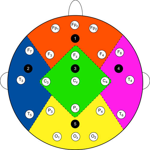
Figure 1.8 shows the position of the electrodes on the cap to receive EEG signals from the brain of the subjects. Different parts of the brain are differentiated with different colors, dotted lines, and also with integers. For instance, integer 1, which is written on the orange part, denotes the frontal part of the brain. This part includes five channels—FP1, FP2, FPz, F3, and F4. The left temporal is denoted by integer 2, and it is highlighted with blue color. This part includes three (3) channels—F7, T3, and T5. Similarly, the central part of the brain is denoted by integer 3, and it is highlighted with green color. This part has 5 channels—Fz, C3, Cz, C4, Pz. The fourth part is the right temporal, which is denoted by integer 4 and is highlighted by pink color. This part constitutes of three (3) channels—F8, T4, T6. Similarly, the last part, which is denoted by integer 5, is the occipital region. This part is highlighted with yellow color, and it consists of five channels—P3, P4, O1, O2, and Oz.
Neural Synchrony Measurement Technique
In this section, we briefly review the synchrony measurement techniques that we have implemented on our data sets, which include phase synchrony, cross-correlation, and coherence.
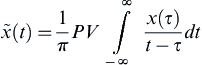
Phase Synchrony (Hilbert Transform)
The oscillation of two or more cyclic signals where they tend to keep a repeating sequence of relative phase angles is called phase synchronization. Synchronization of the two periodic nonidentical oscillators refers to the adjustment of their rhythmicity, that is, the phase locking between the two signals. It refers to the interdependence between the instantaneous phases  and
and  of the two signals
  and
and , respectively. It is usually written as
![]() (1)
(1)
where n and m are integers indicating the ratio of possible frequency locking, and  is their relative phase or phase difference. To compute the phase synchronization, the instantaneous phase of the two signals should be known. This can be detected using analytical signals based on Hilbert Transform.
![]() (2)
(2)
Here z(t) is a complex value, where x(t) is a real time series and  (t) is its Hilbert transform.
The Hilbert transform can be calculated as
 (3)
(3)
Here PV denotes the Cauchy principle value. The instantaneous phase and for both signals can be calculated with the formula
![]() (4)
(4)
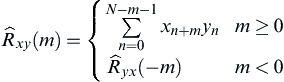
Cross-Correlation
Cross-correlation is a mathematical operation used to measure the extent of similarity between two signals. If a signal is correlated to itself, it is called auto-correlated. If we suppose that x(n) and y(n) (why not S1(t) and S2(t) make a uniform signals suggestion) are two time series, then the correlation between is calculated as
 (5)
(5)
Cross-correlation returns a sequence of length 2∗N − 1 vector, where x and y vectors are of length N (N > 1). If x and y are not of the same length, then the shorter vector is zero-padded. Cross-correlation returns values between −1 and +1. If both signals are identical to each other the value will be 1; if they are totally different to each other then the cross-correlation coefficient is 0, and if they are identical with the phase shift of 180o then the cross-correlation coefficient will be -1 [35].
Magnitude Squared Coherence
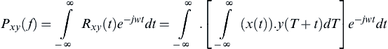
The coherence functions estimates the linear correlation of signals in frequency domain. The magnitude squared coherence is defined as the square of the modulus of the mean cross power spectral density (PSD) normalized to the product of the mean auto PSDs. The coherence  between two channel time series is computed as
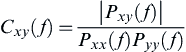 (6)
(6)
For discrete signals  and
and  , cross PSDs (
 ) can be calculated with the given formula:
![]() (7)
(7)
Here, cross spectral density, which is also known as cross power spectrum, is the Fourier transform of the cross-correlation function.
 (8)
(8)
Where  is the cross-correlation of
  and
and  . On the other side, auto PSDs (
 , and
, and  ) for and can be calculated from the auto correlation instead of cross-correlation functions.
![]() (9)
(9)
![]() (10)
(10)
Data Description and Data Filtering
The data sets we are analyzing have been recorded from three different countries of European Union. Specialist at the memory clinic referred all patients to the EEG department of the hospital. All patients passed through a number of recommended tests; MMSE, The Rey Auditory Verbal Learning Test, Benton Visual Retention Test, and memory recall tests. The results are scored and interpreted by psychologists and a multidisciplinary team in the clinic. After that, each patient is referred to the hospital for EEG assessment to diagnose the symptoms of AD. Patients were advised to be in a resting state with their eyes closed during the test. The sampling frequency and number of electrodes for three data sets are all different. Detailed information is as follows.
Database A
The EEG data set A contains 17 MiAD patients (10 males; aged 69.4 ± 11.5 years) and 24 healthy subjects (9 males; aged 77.6 ± 10 years). They all are of British nationality. These data were obtained using a strict protocol from Derriford Hospital, Plymouth, United Kingdom, and has been collected using normal hospital practices. EEG signals were obtained using the modified Maudsley system which is similar to the traditional International 10-20 system. EEGs were recorded for 20 seconds at a sampling frequency of 256 Hz (later on sampled down to 128 Hz) using 21 electrodes.
Database B
This EEG data set was composed of 5 MiAD patients (2 males; aged 78.8 ± 5.6 years) as well as 5 healthy subjects (3 males; aged 76.6 ± 10.0 years). They all are of Italian nationality. Several tests, for instance; MMSE, the Clinical Dementia Rating Scale (CDRS), and the Geriatric Depression Scale (GDS) were conducted to evaluate the cognitive state of the patients. The MMSE result for healthy subjects is 29.3 ± 0.7, whereas for MiAD patients it is 22.3 ± 3.1. EEGs were recorded for 20 seconds at a sampling frequency of 128 Hz using 19 electrodes at the University of Malta, Msida MSD06, Malta.
Database C
This data set consists of 8 MiAD patients (6 males; aged 75 ± 3.4 years) and 3 healthy subjects (3 males; aged 73.5 ± 2.2 years). They all are of Romanian Nationality. The AD patients have been referred by a neurologist for EEG recordings. The time series are recorded for 10 to 20 minutes at a sampling frequency of 512 Hz using 22 electrodes. The signals are notch filtered at 50 Hz. Further details about the data can be found in [51].
For the current study, we have obtained a version of the data that is already preprocessed of artifacts by using independent component analysis (ICA), a blind source separation technique (BSS).
Data Filtering into Five Frequency Bands
EEG time series are classified into five frequency bands. Each frequency band has its own physiological significance.
• Delta (δ: 1 ≤ f ≤ 4 Hz): are characterized for deep sleep and are correlated with different pathologies.
• Theta (θ: 4 ≤ f ≤ 8 Hz): play an important role during childhood. High theta activities in adults are considered abnormal and associated with brain disorders.
• Alpha (α: 8 ≤ f ≤ 12 Hz): usually appear during mentally inactive conditions and under relaxation. They are best seen during eyes are closed and mostly pronounced in occipital location.
• Beta (β: 12 ≤ f ≤ 25 Hz): are visible in central and frontal locations. Their amplitude is less than alpha waves and they mostly enhance during tension.
• Gamma (γ: 25 ≤ f ≤ 30 Hz): are best characterized for cognitive and motor functions.
Bandpass filter is applied to each EEG channel to extract the EEG data in specific frequency bands [F : (F + W)] Hz. Butterworth filters were used (of second order) as they offer good transition band characteristics at low coefficient orders; thus, they can be implemented efficiently [36].
Different Approaches to Compute EEG Synchrony
Different approaches have already been implemented to measure the synchrony between different parts of the brain for Alzheimer patients, MCI patients and healthy subjects. Dauwels et al. [35] have proposed two unique methods to compute synchrony, which they named Local and Global synchrony measures. In the Local synchrony, they computed the synchrony of different regions (left and right temporal, frontal, central, and occipital) separately and then compared the results of one region with the other. In the Global approach, synchrony measures are applied to all 21 channels simultaneously. They named this computation “large-scale synchrony measure” since each region spans several tens of millimeters.
Taking inspiration from these concepts, we have presented advanced and novel approaches to compute EEG synchrony for Alzheimer patients, for all parts of the brain in optimized and narrow frequency bands. In this chapter, we present average and principal components analysis (PCA)–based EEG synchrony measure for Alzheimer and healthy subjects as shown in the Figure 1.9. A detailed description of these methods is provided in the next sections.
Average Synchrony Measure
Average EEG synchrony takes its name because the likelihood of synchronization between two parts of the brain is calculated by computing the average of synchrony measures for all channel pairs between two respective parts. This means that first we apply neural synchrony measurement technique on each channel pair (time series of two channels) of two different regions for all frequency bands and then we take the average of those results.
For instance, we apply phase synchrony measure on each channel pair of left and right temporal ((F7–F8), (F7–T4), (F7–T6), (T3–F8), (T3–T4), (T3–T6), (T5–F8), (T5–T4), (T5–T6)) and then we take the average result of right temporal–left temporal. Similarly, we compare the left temporal with frontal ((F7–FP1), (F7–FP2), (F7–FPz), (F7–F3), (F7–F4), (T3–FP1), (T3–FP2), (T3–FPz), (T3–F3), (T3–F4), (T5–FP1), (T5–FP2), (T5–FPz), (T5–F3), (T5–F4)), left temporal–central ((F7–Fz), (F7–C3), (F7–Cz), (F7–Pz), (T3–Fz), (T3–C3), (T3–Cz), (T3–C4), (T3–Pz), (T5–Fz), (T5–C3), (T5–Cz), (T5–C4), (T5–Pz)), and left temporal–occipital ((F7–P3), (F7–P4), (F7–O1), (F7–O2), (F7–Oz), (T3–P3), (T3–P4), (T3–O1), (T3–O2), (T3–Oz), (T5–P3), (T5–P4), (T5–O1), (T5–O2), (T5–Oz)).
Working on the same lines, we compare the right temporal (F8, T4, T6) with rest of the brain area. For instance, we apply phase synchrony measure on each channel pair of right and left temporal ((F8–F7), (T4–F7), (T6–F7), (F8–T3), (T4–T3), (T6–T3), (F8–T5), (T4–T5), (T6–T5)) and then we take the average result of right temporal–left temporal. Similarly, we compare the right temporal with frontal ((F8–FP1), (F8–FP2), (F8–FPz), (F8–F3), (F8–F4), (T4–FP1), (T4–FP2), (T4–FPz), (T4–F3), (T4–F4), (T6–FP1), (T6–FP2), (T6–FPz), (T6–F3), (T6–F4)), right temporal–central ((F8–Fz), (F8–C3), (F8–Cz), (F8–Pz), (T3–Fz), (T4–C3), (T4–Cz), (T4–C4), (T4–Pz), (T6–Fz), (T6–C3), (T6–Cz), (T6–C4), (T6–Pz)), and right temporal–occipital ((F8–P3), (F8–P4), (F8–O1), (F8–O2), (F8–Oz), (T4–P3), (T4–P4), (T4–O1), (T4–O2), (T4–Oz), (T6–P3), (T6–P4), (T6–O1), (T6–O2), (T6–Oz)).
The same procedure has been repeated for rest of the synchrony measures, that is, cross-correlation and coherence. After getting the results, we compare the neural synchronization of AD patients and healthy subjects, for all three measurement techniques (phase synchronization, cross-correlation and coherence), by Mann–Whitney U test.
PCA-Based Synchrony Measure
The basic purpose of PCA is to reduce the dimensionality of a data set to convert it to uncorrelated variables providing maximum information about a data point, eliminating interrelated variables. In other words, it transforms highly dimensional data set (of m dimensions) into low-dimensional orthogonal features (of n dimension), where n < m.
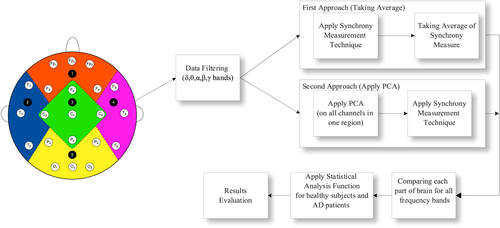
In this method, instead of applying synchrony measurement techniques directly on the filtered data, first we apply the PCA technique on all channels of one region. This eliminates any redundant information that a region might provide. For instance, we apply PCA on all three channels of left temporal (F7, T3, T5) and, consequently, it provides a single signal without any redundant information. It is noteworthy here that still we have a signal into five narrow frequency bands (δ, θ, α, β, γ) for each part. This means that for left temporal, after the application of PCA on three channels (F7, T3, T5), we have a single signal, say LT, for all these frequency bands: LTδ, LTθ, LTα, LTβ, LTγ. Similarly, after applying PCA to right temporal (RT), we have the following signals: RTδ, RTθ, RTα, RTβ, RTγ. For frontal, central, and occipital, the signals are as (Fδ, Fθ, Fα, Fβ, Fγ), (Cδ, Cθ, Cα, Cβ, Cγ), and (Oδ, Oθ, Oα, Oβ, Oγ) respectively.
After the application of PCA, now we have a single comprehensive signal in five frequency bands in each part. Proceeding toward the findings of neural synchronization, we apply the neural synchrony measure, say phase synchrony, on EEG time series of two regions. We calculated phase synchrony between left and right temporal ((LTδ–RTδ), (LTθ–RTθ)–, (LTα–RTα), (LTβ–RTβ), (LTγ–RTγ)), left temporal–frontal ((LTδ–Fδ), (LTθ–Fθ)–, (LTα–Fα), (LTβ–Fβ), (LTγ–Fγ)), left temporal–central ((LTδ–Cδ), (LTθ–Cθ)–, (LTα–Cα), (LTβ–Cβ), (LTγ–Cγ)), and left temporal–occipital ((LTδ–Oδ), (LTθ–Oθ)–, (LTα–Oα), (LTβ–Oβ), (LTγ–Oγ)).
Similarly, we have compared right temporal with the rest of the brain areas; right temporal–left temporal ((RTδ–LTδ), (RTθ–LTθ)–, (RTα–LTα), (RTβ–LTβ), (RTγ–LTγ)), right temporal–frontal ((RTδ–Fδ), (RTθ–Fθ)–, (RTα–Fα), (RTβ–Fβ), (RTγ–Fγ)), right temporal–central ((RTδ–Cδ), (RTθ–Cθ)–, (RTα–Cα), (RTβ–Cβ), (RTγ–Cγ)), and right temporal–occipital ((RTδ–Oδ), (RTθ–Oθ)–, (RTα–Oα), (RTβ–Oβ), (RTγ–Oγ)).
The same procedure has been repeated for rest of the synchrony measures, that is, cross-correlation and coherence. After getting the results, we compare the neural synchronization of MiAD patients and healthy subjects for all three measurement techniques (phase synchronization, cross-correlation and coherence) by Mann–Whitney U test.
Statistical Analysis
To investigate whether there is a significant difference between the EEG signals of MiAD patients and control subject and also to prove the probable significance of our proposed methodology, we apply the Wilcoxon rank sum (Mann–Whitney) test on our data sets. The rank sum function is a nonparametric test that allows to check whether the statistics at hand, in our case synchrony results, take different values from two different populations. Lower p-values indicate higher significance in terms of large difference in medians of two populations.
Results are compared in two different perspectives:
1. Investigating three different synchrony measures at a time will help us to compare which measure works better for EEG signals.
2. Second, we are able to compare two different methods for three synchrony measures and for three different data sets.
Results and Discussion
The aim of the present study is to find the relationship of EEG synchronization with AD, and thus to explore further dimensions in the disconnection theorem of cognitive dysfunction in AD. And also, we aim to propose a better method to detect any change in EEG synchrony that can be considered as a biomarker for the early detection of AD.
First we discuss all three synchrony measures with PCA based method. As shown in the Table 1.1, the p-values for cross-correlation in the RT-C region are 2.47 x 10⁻⁴, 1.46 x 10⁻⁴, 0.009 for delta, theta, and alpha bands, respectively. In the LT-O region, the smallest p-values for delta and theta bands are 8.50 x 10⁻⁵ and 6.8 x 10⁻⁵ respectively. The second best measure that has given us remarkable results is phase synchrony, where we get 0.0067, 0.0403, and 0.0585 p-values for delta, theta, and alpha bands, respectively, in the RT-C region. We get 0.0041 and 0.0271 p-values for delta and alpha bands, respectively, in the LT-O region. Lastly, the coherence function shows significant results in the RT-C region for delta band, p-value = 0.0378, and in the LT-O region with p-values 9.8 x 10⁻⁴ and 0.05 for delta and alpha bands, respectively. Coherence function does not provide significant results and hence contradicts Bahar theory [37], where the control group showed higher values of evoked coherence in delta, theta, and alpha bands in the left frontoparietal electrode pairs compared with AD patients.
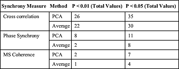
Similarly, we have found 8 significant values below 0.01 (p < 0.01) and 11 significant values below 0.05 (p < 0.05) for the PCA-based method whereas only 2 values below 0.01 (p < 0.01) and 8 values below 0.05 (p < 0.05) in case of the Average method for phase synchrony measure. Similarly, for cross-correlation measure, although the difference is not very high, the PCA method still has shown more significant values. For example, the number of p-values below 0.01 (p < 0.01) are 26 whereas almost all 35 values are below 0.05 (p < 0.05); on the other hand, for the Average method, 22 values are below 0.01 whereas 30 values are below 0.05 (p < 0.05), as shown in the Table 1.2. As aforementioned, coherence function does not perform better compared with other two synchrony measures, but again we found more significant results in case of the PCA method (2 values below 0.01 and 7 values below 0.05) compared with the Average method, wherein we found only one significant value below 0.01 and 7 significant values below 0.05.
Table 1.1
P-Values at Different Frequency Bands in Different Brain Connections
| Synchrony Measure | Brain-Connections | Frequency regions | P-values |
| Cross Correlation | RT-C | Delta (δ) | 2.47 × 10⁻⁴ |
| Theta(θ) | 1.46 × 10⁻⁴ | ||
| Alpha(α) | 0.009 | ||
| RT-O | Delta (δ) | 6.9 × 10⁻⁵ | |
| Theta(θ) | 2.7 × 10⁻⁵ | ||
| Alpha(α) | 0.0029 | ||
| RT-F | Delta (δ) | 5.01 × 10⁻⁴ | |
| Theta(θ) | 6.8 × 10⁻⁵ | ||
| Alpha(α) | 0.0062 | ||
| LT-C | Delta (δ) | 4.3 × 10⁻⁵ | |
| Theta(θ) | 3.8 × 10⁻⁵ | ||
| Alpha(α) | 0.0192 | ||
| LT-O | Delta (δ) | 8.5 × 10⁻⁵ | |
| Theta(θ) | 6.8 × 10⁻⁵ | ||
| Alpha(α) | 0.0052 | ||
| LT-F | Delta (δ) | 2.2 × 10⁻⁴ | |
| Theta(θ) | 5.4 × 10⁻⁵ | ||
| Alpha(α) | 0.0091 | ||
| LT-RT | Delta (δ) | 3.3 × 10⁻⁴ | |
| Theta(θ) | 6 × 10⁻⁵ | ||
| Alpha(α) | 0.0253 | ||
| Phase Synchrony | RT-C | Delta (δ) | 0.0067 |
| Theta(θ) | 0.0403 | ||
| Alpha(α) | 0.05 | ||
| RT-O | Delta (δ) | 0.0041 | |
| Alpha(α) | 0.0271 | ||
| Coherence | RT-C | Delta (δ) | 0.0378 |
| RT-O | Delta (δ) | 0.0378 | |
| Alpha(α) | 0.0192 |
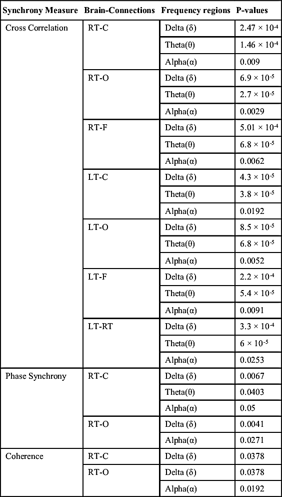
Results revealed that cross-correlation (xcorr) synchrony in right temporal–occipital (RT–O) for theta (θ), alpha (α), and beta (β) ranges provides an optimal information for the early diagnosis of Alzheimer patients. Also, phase synchrony measure in left temporal–frontal (LT–F) and left temporal-right temporal (LT–RT) regions provides significant information for theta (θ) and beta (β) ranges. The provided results support our hypothesis that a decrease in synchronization between temporal regions have a direct link with the progression of AD. These findings will help clinicians for the early diagnosis of AD patients.
Conclusion
This chapter has presented a framework for the early diagnosis of NDDs using signal processing and signal classification techniques. The problem with the NDDs is that they are incurable, hard to detect at earlier stages because of nonobvious symptoms, and also hard to discriminate at later stages because of pattern similarities of different NDDs. Because there is no single authentic remedy available for such diseases, scientists find a lot of interest in finding those hidden patterns that can help us in the early diagnosis of NDDs. This chapter has highlighted the importance of machine learning and signal processing in the early diagnosis of life-threatening diseases such as Alzheimer, Parkinson, Huntington, and ALS. In this thesis, we have presented the issues with the early diagnosis of NDDs and also with their possible solutions. The analysis and classification of gait signals is presented using a set of well-known classifiers—linear, nonlinear, and Bayes. Results are presented and elaborated from various dimensions using more than one performance evaluation technique. In addition, we have proposed and demonstrated a novel idea of combining classifiers to improve the classification accuracy. The latter half of the thesis presented the implementation of neural synchrony measurement techniques using EEG signals to calculate synchronization in different parts of the brain for Alzheimer and non-Alzheimer patients. The chapter has presented novel and significant findings that can be used in clinical practices for the early diagnosis of NDDs.
..................Content has been hidden....................
You can't read the all page of ebook, please click here login for view all page.