Chapter 7: Modeling Payer Data

Chapter Summary. 159

Chapter Learning Goals. 159

Payers. 160

Payer Anamatics. 161

Payer Data. 162

Payer Systems and Sources of Data. 162

Payer Systems Process. 162

Claim Forms. 163

Experiential Learning Activity - Claim Forms Billing. 164

Experiential Learning Activity: Claims Adjudication Processing. 165

Electronic Data Interchange. 167

EDI Structure. 171

Experiential Learning Activity: EDI Translation. 173

SEMMA: Model 174

Model Process Step Overview.. 174

Model Tab Enterprise Miner Node Descriptions. 175

Experiential Learning Application: Patient Mortality Indicators. 177

Model Summary. 197

Experiential Learning Application: Self-Reported General Health. 197

Executive Summary. 197

Learning Journal Reflection. 199

The purpose of this chapter is to develop data modeling skills using SAS Enterprise Miner, and with respect to the Model capabilities within the SEMMA process. The chapter explores modeling with the decision tree model. This chapter also includes experiential learning application exercises on patient mortality indicators and self-reported general health. The focus of this chapter is detailed in Figure 7.1.

Figure 7.1: Chapter Focus – Model

●       Describe the Model process steps

●       Understand payer-level data sources

●       Develop data modeling skills

●       Apply SAS Enterprise Miner model data functions

●       Master the decision tree model

Payers include insurance agencies and third-party payment processors. Typically, payers are separated into categories of commercial payers, governmental payers, and third-party payers. The most commonly known type of payer includes commercial payers such as UnitedHealth Group and Blue Cross Blue Shield. Government payers include Medicare and Medicaid, which will be covered further in Chapter 8. Third-party payers include self-insured health plans by an employer and other insurance providers such as health costs covered through care insurance or workers’ compensation (PHDSC, 2007). In some cases, providers are setting up independent health plans due to the shift in value-based healthcare to maximize returns. Hospitals could partner with a physician-owned health plan in order to share the cost savings from the value-based care. Hospitals and providers continue to work in hand with insurers to identify high-cost or high-risk patients and to improve coordination of care (Livingston, 2016).

Government insurances were originally designed out of a need, due to a lack of coverage available in commercial markets. Medicare was enacted for people over 65, since those over 65 were three times more likely to use medical services, and the costs were unaffordable for both patients and insurers. Medicare is a federal program in the U.S. and is paid for through payroll taxes. By pooling resources, it enables the protection of individuals in the event of a high-cost healthcare requirement. In addition, there are no exclusions to the program based on age beyond the minimum age of 65, health status, or income. By contrast, commercial insurance aims to avoid risk in order to ensure that a profit is made and the company remains in business. The for-profit aspect allows commercial insurers to exclude those of high risk or high cost, and create barriers to payment of all claims (Archer and Marmor, 2012). TRICARE is another government-based U.S. healthcare program for uniformed service members and families and covers general healthcare, prescriptions, and dental plans. The program is managed through the Defense Health Agency and seeks to provide a world-class healthcare system for its over 9.4 million participants. TRICARE offers plans that meet the ACA requirement to maintain minimum coverage (Tricare, 2017). Another related program is the Civilian Health and Medical Program of Veterans Affairs (CHAMPVA), and covers the majority of health expenses. To be eligible for CHAMPVA, members cannot be eligible for TRICARE, and the program has requirements for those with disabilities. CHAMPVA is managed through the Veterans Health Administration and has over 1,700 locations with over 8.7 million participants. Veterans programs also meet the ACA requirements, and veterans might choose among plans including from the VA and TRICARE (VFW, 2017; VA.gov, 2017).

Commercial insurance models typically have a model of a Health Maintenance Organization (HMO), Preferred Provider Organization (PPO), or Self-Funded Plan. An HMO model uses a primary care physician (PCP) to act as a main point of contact for a patient’s care and refers the patients to specialists or other plans of care as appropriate. The PPO model permits patients to see different providers directly and, as a result, usually carry a higher premium. Both HMO and PPO plans typically have an assigned network of providers with which they contract and negotiate rates. Both HMO and PPO plans also typically pay providers per service rendered or also known as a fee-for-service model (MedicalBillingandCoding, 2017). A self-insured health plan, also known as a self-funded plan, is where the employer pays the financial cost for the healthcare for their employees. With an HMO or PPO plan, a monthly fixed premium is paid for each member, and the insurer pays the financial cost of healthcare. Self-funded plans might represent up to half of all commercial plans. Employers choose this type of plan to allow more customization of providers and coverage, maintain control, and reduce regulations and taxes. Disadvantages include financial risk that can be unpredictable. The self-funded type of plan can be challenging for small businesses or those with a high-cost population. Typically, an employer will contract with an existing insurer to administer the self-funded plan, giving a similar network and coverage options with the main difference of financial risk. Over 90% of employers with 5,000 of more workers are self-funded or partially self-funded (SIIA, 2015; Kaiser Family Foundation, 2016).

In the U.S., the largest commercial health insurers collect over $700 billion in annual premiums, and in 2017 the average annual family premiums were $18,764 (NCSL, 2017). Top insurers in the U.S. include UnitedHealth Group, Kaiser Foundation, WellPoint, Aetna, Humana, Cigna, Highmark, and Blue Cross Blue Shield (BCBS) within various state organizations such as BCBS of California (Heilbronn, 2017; NCSL, 2017). There have been previous attempts between health insurers to pursue mergers and acquisitions within the industry. Anthem offered $48 billion to acquire Cigna, and Aetna sought to acquire Humana for $34 billion. In both cases, federal judges blocked the acquisitions after U.S. Justice Department officials believed the combinations would lead to increased premiums due to reduced competition. Insurance companies argued that these would help them negotiate better prices from pharmaceutical companies and hospitals for their customers. The companies are still considering options for appeals, pending potential changes in federal administration, and pursuing various litigation with regard to termination fees and damages due to the failed mergers. With potential changes also planned to the Affordable Care Act and related U.S. healthcare legislation, many insurers are in a wait-and-see mode, holding on to their cash stockpiles and determination options for their investment (Tracer et al., 2017; Murphy, 2017). Other healthcare organizations are moving forward, with CVS proposing a nearly $70 $1billion merger with Aetna (Ramsey, 2018). Cigna acquired Express Scripts, a pharmacy benefit and healthcare management company for $67 billion. Walmart is reportedly reviewing their own options for acquiring Humana health insurance (Pearson, 2018). Walgreens Boots Alliance and wholesale drug distributor AmerisourceBergen have met to discuss a potential $25 billion deal. Other competitors including Amazon, Kroger, and Albertsons have been exploring varying strategies including acquisitions, mergers or alliances with healthcare payers and intermediaries (Hirsch and Sherman, 2018).

Health anamatics has great potential to transform payer cost efficiency and coverage. Although analytics and informatics have been used by payers for many years for actuarial purposes, usage in other areas of payer operations has varied. Payers are currently focusing on patients, providers, and customers to improve savings. Payers also review financial and operational measures such as forecasting, operations, and fraud monitoring. On the patient side, payers have attempted to identify patients that will have future high costs, in order to increase interventions through preventative care. To assist providers, payers have focused on pay-for-performance programs and fraudulent billing. Similar to the providers, most payers are at stage 2 – localized analytics, of the five levels of analytics capability. Although localized analytic capabilities exist, a more complete organizational strategy is still in development, and organizational data warehouse and common analytics toolsets are not prevalent. Payers such as UnitedHealthcare through the acquisition of Ingenix as a subsidiary have developed more advanced analytics capabilities. Payers are also seen as being in an ideal position to use health anamatics given the large amounts of claims and transaction data available to them (Cheek, 2014)

Payers also generate and collect large amounts of data on patients, providers, and outside sources. Common payer systems include claims, population health management, financial and billing. As part of population health management, insurance sponsored or run personal health records and screenings also collect and store information about patients. Following the screening, wellness systems are offered through insurance carriers such as Florida Blue to promote healthier lives through eHealth education and incentives. Insurers also have an incentive to offering these programs as part of their plans aimed at reducing incurred healthcare costs. Insurers also collect personal data such as medical records and health history when reviewing coverage applications and claims. For example, some insurers might even access social media data to use while reviewing a claim. Although several payer systems are developed in-house, software vendors of provider systems also develop payer systems. Epic, a company known for their EHR software, has a product called Tapestry for managing health insurance. Features include enrollment verification, member portals, care management to improve health outcomes, customer relationship management modules, utilization management, and claims adjudication, processing and billing (Epic, 2017).

Another well-known company for claims processing is TriZetto, which permits electronic claims processing. Trizetto has software edits to reduce errors and improve payments. It creates secondary billing for claims with additional insurance payers, sends electronic bill remittances, and converts image files to HIPPA compliant EDI formats. Trizetto has built-in business intelligence and analytics for reports and tracking claims data for improving decision-making. In 2014, Cognizant announced a $2.7 billion acquisition of privately held Trizetto. The combined company includes 350 health payers and 180 million covered lives within the U.S. (Cognizant, 2014; Trizetto, 2017). McKesson also offers supporting software for payers such as ClaimsXten, an auditing software to improve accuracy of payments, increase auto-adjudication, convert between ICD 9 and 10 codes, reduce administrative costs, such as through identification of waste and abuse items, and local coverage decisions (McKesson, 2017).

Health claim processing varies by vendor and plan, with advantages for each method. Overall, a common system framework exists despite the individual process differences. The first layer includes the data storage, contained within a database management system. The database stores the claims data, provider data, and member data. The system should contain a set of reporting tools for making business decisions, producing regulatory reporting, and providing customers with information. A system should contain a processing engine for developing rules to adjudicate or process claims, including automatic adjudication. The system should also provide a method for customization and modifications of benefits and rules, which is due to the increasing complexity of health claims processing (TM Floyd, 2006).

A typical process would begin first with the completion of a medical treatment. The medical treatment would then be followed by a claim submission to the insurer. The claim form might be mailed on paper or sent electronically. The claim form can be scanned and read or manually entered. The health plan will then review the claim to determine whether payment should be made. The payment determination and amount is called adjudication. During adjudication, the health plan will also check the patient benefits and eligibility for services. The provider will also be verified for processing and payment terms. Further checks for other insurance coverage will be made and various quality checks conducted, such as a duplicate claims check. Health plans might also reject the claim or deny the claim without payment. Once adjudication is complete and payment determinations made, an Explanation of Benefits (EOB) will be generated and sent to the insured, which is typically the patient (TM Floyd, 2006).

Two primary paper claim forms are used for billing payers: the CMS-1500 previously known as an HCFA (Healthcare Financing Administration) form for outpatient claims, and a CMS-1450 previously known as a UB-92 (uniform billing) form for inpatient claims. Electronic claims use Electronic Data Interchange (EDI) transactions, which are standardized through HIPAA. The HIPAA 837 is the equivalent EDI transaction for the CMS-1500 and CMS-1450 paper forms (CMS, 2014; CMS, 2016b). EDI transactions for claims were modeled after the paper forms with additional capabilities. Within the forms and EDI transactions there are a number of common insurance billing terms. Table 7.1 includes a brief summary of key terms.

Table 7.1: Claims Terminology

Term(s)	Definition/Example
Guarantor, Health Plan, Payer	This is the financially responsible party for the claim, such as Aetna.
Subscriber, insured party, enrollee, member, beneficiary	This is the patient that represents the claim. Historically, this might have included the parent as the subscriber. However, most health plans now bill using the patient information only.
Member number, policy number, insurance ID	This is the unique identifier for the patient. Historically, this might have been a social security number. However, most health plans now assign each patient a unique identifier that does not identify the individual patient.
Group number	This is the unique identifier of the coverage group. Typically, this number is the same for all employees of a given employer and identifies the coverage and benefits.
Adjudication	This is the process of reviewing and paying the claim by the insurer. The claim can be automatically adjudicated or require a human review to determine coverage and payment.
Explanation of benefits (EOB), remittance advice	The explanation of benefits is provided to the patient following insurer adjudication. This form explains the charges from the provider and what was covered or paid by the insurer after adjudication.
Billed amount	This is the original amount billed by the provider for the service(s) rendered, and can include one or more services, such as an office visit, medical supplies, and so on.
Allowed amount	This is the maximum amount permitted for the service(s) as per the contract between the insurer and provider.
Contractual Adjustment	This is the difference between the billed amount and the allowed amount per the contract between the insurer and provider.
Coordination of benefits, crossover or piggyback claims	This can occur if a patient has more than one coverage or priority coverage. For example, a claim can be first paid by Workman’s Compensation as the primary payer if the employee was injured at work. Then any remaining amounts can be covered by the employee’s commercial insurance as the secondary payer.
Copay, coinsurance, deductible, out of pocket amount	These are the amounts the patient is responsible for, even if the claim is paid by the insurer. These help offset the monthly premium costs and are referred to as shared patient responsibilities.

To learn more the claims process and claim forms, we will review claim billing and payment processing examples using the paper-based forms.

Claim Forms Billing

Description: CMS-1500 is the most commonly used claim form, and is used for professional claims such as physician office visits. Navigate to http://CMS.gov, search for “CMS-1500,” and open the CMS-1500 form. For this activity, you will practice completing the paper-based forms. The form is completed through a series of numbered boxes, 1-33. Some boxes have subparts such as 1a. The form completion order is like reading a page, left to right, top to bottom. Complete the form using sample data for yourself as the patient. Some boxes will require a code lookup. In box 21, you will need to enter the ICD-10 diagnosis code. In box 21 d., you will need to enter the CPT/HCPCS code. There is a more detailed CMS-1500 form instruction available for field by field assistance. CMS-1500 Form: https://www.cms.gov/Medicare/CMS-Forms/CMS-Forms/Downloads/CMS1500.pdf CMS-1500 Form Instructions: http://www.cms.gov/Regulations-and-Guidance/Guidance/Manuals/Downloads/clm104c26.pdf ICD-10 Lookup: https://www.cms.gov/Medicare/Coding/ICD10/2018-ICD-10-PCS-and-GEMs.html http://www.icd10data.com HCPCS Fee Lookup: http://www.cms.gov/apps/physician-fee-schedule/overview.aspx

 

Claims Adjudication Processing
Description: For this experiential learning activity, you will take the role of a claims adjudicator. The claim is adjudicated following the payer receipt of the paper claim form from the provider. In order to adjudicate the claim properly, coverage information has been provided. Calculate the amounts following the review.
Reimbursement Key Terms Summary
Eligibility: Span of insurance coverage based on service date. Premium: Monthly payment for insurance. Copay: Fixed amount due at time of each service regardless of deductible/OOP, can vary by type or location. Deductible: Direct amount of payment before insurance begins. Coinsurance: Percentage of allowed amount payment after deductible is met. Out-of-Pocket Maximum: The highest cumulative payment in a calendar year, generally deductible, co-pay and co-insurance all count toward your out-of-pocket maximum. Contracted Payment: Amount your insurance has agreed to pay the provider of care.
Claim Adjudication
Benefit Coverage Details: Eligibility Dates: 1/1/2018 – 12/31/2018 Plan: Florida BlueCare Everyday Health Premium: $325 Per Month Allowed Amount - Contracted Payment Rate: 80% of Billed Copay: $0 Preventative (e.g. immunization) / $20 Primary Care Provider / $35 Specialist / $75 ER Deductible: $500 Per Person / $1,600 Per Family Coinsurance: 10% of the Allowed Amount (after deductible is met) Out-of-Pocket Maximum: $2,500 Per Person / $5,000 Per Family
Claim Adjudication
2018 Beneficiary Records (Totals YTD): Member 11111111: •      Deductible Individual / Family: $0 / $0 •      OOP Individual / Family: $0 / $0 Member 22222222: •      Deductible Individual / Family: $500 / $1600 •      OOP Individual / Family: $2500 / $5000 Member 33333333: •      Deductible Individual / Family: $100 / $100 •      OOP Individual / Family: $20 / $20
Claim Adjudication
Claim # 1000 Member 11111111 Service Date 3/1/2018 Service/Procedure Office Visit Billed Amount $100 Allowed Amount   Not Covered Amount   Copay Amount   Deductible Amount   Coinsurance Amount   Patient Responsible   Insurance Responsible
Claim # 1001 Member 22222222 Service Date 12/5/2017 Service/Procedure Office X-Ray Billed Amount $150 Allowed Amount   Not Covered Amount   Copay Amount   Deductible Amount   Coinsurance Amount   Patient Responsible   Insurance Responsible
Claim # 1002 Member 33333333 Service Date 5/15/2018 Service/Procedure Specialist Visit Billed Amount $250 Allowed Amount   Not Covered Amount   Copay Amount   Deductible Amount   Coinsurance Amount   Patient Responsible   Insurance Responsible

 

Now that you are familiar with the paper-based forms for claims billing, we will cover the alternative electronic method known as EDI, which captures a similar set of data as the paper form and includes the ability to send additional information that is not included in the paper forms. Electronic Data Interchange (EDI) is the computer-to-computer exchange of information that uses international standards. Large retailers such as Wal-Mart, the automotive industry, and the healthcare industry all use EDI. EDI uses computerized technology to exchange data and improve processing efficiencies, delivery times, reliability, and quality over existing methods. EDI allows for standardized and efficient transmission of data between organizations. EDI is included as part of the Health Insurance Portability and Accountability Act (HIPAA) standards to facilitate administrative cost savings and efficiencies. HIPAA required the Secretary of Department of Health and Human Services to adopt standards to support the electronic exchange of administrative and financial healthcare transactions primarily between healthcare providers and plans. Transaction standards and specifications were adopted by the Secretary to enable health information to be exchanged electronically. Implementation guides for each standard have been produced at the time of adoption, and consistent usage of the standards (including loops, segments, and data elements) across all guides is mandatory to support the Secretary’s commitment to standardization (Woodside, 2013).

The typical healthcare data process flow involves setting the standard transaction set in batch mode through a file transfer protocol (FTP) or other similar transport method over a Value-Added Network (VAN). The process typically results in a transmission/receipt occurrence once per day. The alternative would be a real-time transmission/receipt resulting in multiple transmission/receipts per day and would use HTTP or a similar protocol as the transport method. The EDI x12 standard is then converted to XML through a variety of third-party applications or custom-built software. The XML data is then stored in a database, typically as a character large object (CLOB). Existing applications that need to interface with the various EDI transactional data (such as billing systems, claims systems, membership systems, authorization systems, and financial systems), typically cannot read EDI or XML. This results in a secondary conversion to a fixed file format readable by the source system. The data is then stored within the source system for use, resulting in data redundancy within internal systems. For EDI transactions responses (such as a 271, 277, 278, and 835), the process repeats. The source system produces a file in a fixed file format. The file is then converted to XML, which is then converted to the EDI x12 standard (Woodside, 2013).

A clearinghouse, which is an intermediary between providers and health plans, might be used. The typical role of a clearinghouse is to receive EDI transactions from the provider and payer, convert them to the appropriate format, and send them on to the appropriate party. A clearinghouse might take non-HIPAA formatted data and translate it to the standard HIPAA EDI format. A clearinghouse might also run quality or edit checks and analytics on the transactions. Typically, a per transaction fee is assessed by the clearinghouse. A clearinghouse is permitted to transmit PHI, which is considered one of the covered entities under HIPAA. Change Healthcare is one of the largest clearinghouses in the U.S. with over 2,100 payer connections, 5,500 hospitals, and 800,000 physicians. In the latest fiscal year, Change Healthcare processed over 12 billion healthcare transactions and $2 trillion in claims (Change Healthcare, 2017).

In an effort to reduce the costs of healthcare, which in the U.S. has averaged double the inflation rate per year since the 1970s, EDI standards were created as part of the 1996 HIPAA act. The U.S. is not alone in these efforts. China has also implemented measures to promote EDI, including policies and infrastructure investment. Problems confronting healthcare organizations include increasing costs and inefficiencies in resources. Hospitals began using EDI to communicate with other hospitals, suppliers, insurance companies, and banks. The relatively limited EDI presence is explained by high EDI start-up costs as compared with labor, unfamiliar new relationship-making, and technical infrastructure and complexity. A New Jersey state study, the HINT project, estimated the cost savings from the application of computerized systems. Their findings included estimates that 17% of costs are related to processing, and a minimal reduction in those costs would amount to several billion dollars across the industry. Most payers have already put significant investment into computer technology and can further tap into EDI. One of the most detailed and comprehensive analysis for EDI standards was created by Workgroup for Electronic Data Interchange (WEDI). A large number of estimates were provided and included pilot projects. WEDI mentioned that although estimated savings might not result in hard-dollar savings, it will allow for efficiency to be improved and resources to be re-allocated to improve quality, care, and service. Additional studies list benefits, which include near-term reduction of paperwork and a long-term potential to use information technology to improve quality and cost effectiveness of healthcare. System data standards integrated across parties will allow for improved accuracy, reliability, and data usage (Woodside, 2007b).

As part of the HIPAA legislation, a set of approved EDI transactions was developed to simplify processing and reduce costs. The transactions were developed in compliance with ANSI standards and some documentation includes the ANSI prefix. EDI is popular across many different industries (such as finance and manufacturing) with different transaction types and was applied similarly to healthcare. The standard set includes:

Table 7.2: EDI Transactions

Category	Transaction	Description
Authorization	278	Referral certification and authorization. This is used to request prior authorization for a service and provider referral to ensure payment. Precertification or preauthorization is the prior approval by the payer of a certain action to be taken by the provider during treatment. The claim might be denied if authorization is not requested prior to the service. EDI reduces time spent by the payer contacting one another or the provider. Additional time is reduced by documenting and/or entering data received manually. Assuming 30% referrals, admissions and emergency room visits require review/approval; the payer savings from using the EDI 278 transaction is $0.81 to $1.23 per transaction, with provider savings of $0.65 to $0.98 per transaction.
Claims	837	Claims or equivalent encounters and coordination of benefits. The 837 is used for billing the claim, which is similar to the paper form CMS-1450 and CMS-1500. The 837 might have an associated sub-designation, such as 837-I or 837-P, which is a designated institutional or professional claim to match with the same billing of CMS-1450 (institutional claims) and CMS-1500 (professional claims). Claims transactions are simplified through EDI. Information can be entered and transmitted electronically from the provider to the payer. Claim information can be re-sent easily. Re-sent information includes claims corrections and adjustments. The estimate of payer savings ranges from $0.50 to $1.50, minus a transaction cost of $0.17. The provider cost per transaction for physician claims varies from $0.51 to $1.96, with hospital claims from $0.11 to $1.07. Coordination of benefits transactions enables electronic transmission on a single claim. The cost savings potential for payers is $0.22 per transaction. The savings for providers is $0.95 to $1.16 per transaction, based on savings by not identifying, copying, and re-submitting remittances from one payer to another.
Claims – Additional Information	275	Patient Information in Support of a Health Claim or Encounter. The 275 is used for attaching electronic information such as clinical information, lab reports, emergency department, rehabilitative services, ambulance services, and medications. This is for supplemental information not included on the 837 EDI transaction.
Claims - Status	276-277	Claim status inquiry (276) and response (277). The 276-277 is a paired transaction to check on the payment status of a claim. The 276 is sent by the provider to the insurer, and the insurer returns a 277 with the current claim status. In the past, providers might have called on the telephone and waited on hold while the status of the claim was checked. Now they can have real-time updates as needed. Claims status transactions typically are received by mail or phone. It is estimated that public and private healthcare payers receive over 60 million claim status inquiries per year, and EDI is estimated to save payers $1.06 to $2.72 net per inquiry, and save providers $3.56 to $3.88 per inquiry.
Claims - Response	835	Remittance and payment advice, which is known as an Electronic Remittance Advice (ERA). The 835 is used to provide the explanation of benefits and payment and describe how the claim was adjudicated and provides details about the claim payments. Payment and remittance transactions include transfer of funds typically by check, and the explanation of the benefit payments from the payer. Potential savings include electronic remittance and electronic funds transfer transaction. The savings result from the elimination of postage and handling. The manual costs of processing a remittance and payment range from $0.45 to $1.00, and the costs of processing under EDI are $0.11 to $0.35. The net savings range between $0.10 to $0.89. Approximately $73,432 can be saved per year per hospital, and $1,918 in savings per year per physician practice.
Membership - Eligibility	270-271	Eligibility benefit inquiry (270) and response (271). The 270-271 is a paired transaction to check on the eligibility and benefits of the patient. The 270 is sent by the provider to the insurer, and the insurer returns a 271 with the current claim status. In the past, providers might have had to call by telephone and wait on hold to have the status of eligibility checked. Now they can have real-time updates as needed. A patient might not know their co-pay amount, and a provider can easily verify the amount. Eligibility transactions allow confirmation of an individual's eligibility for healthcare services payment by a third party, as well as a determination of benefit coverage including patient liabilities. An estimation of 150 million transactions occur each year, primarily by telephone. The savings estimated for payers is of $0.50-1.00 per inquiry. The savings estimated for providers is $1.10 to $2.09 per inquiry.
Membership - Payment	820	Health plan premium payments. The 820 is used to make monthly payments for the insurance enrollment, which is typically the set of employees.
Membership - Enrollment	834	Enrollment and unenrollment in a health plan. The 834 is to add to or remove from monthly membership in the insurance, which typically occurs as employees are hired and leave each month.
Pharmacy	NCPDP 5.1	Retail drug claims, coordination of drug benefits, and eligibility inquiry. NCPDP is used for billing pharmacy services such as at Walgreens. Electronic prescribing (e-prescribing) savings are estimated at $27 billion per year in the U.S. Savings are due to reduced errors, improved efficiency, and easier access to payer drug formularies or approved drugs when prescribing. Also, savings result from the ability to substitute lower cost generic drugs or formulary options when available (Porterfield et al., 2014).

 

To review the EDI transaction structure, first picture a blank text file. Then to complete a transaction, within the text file, you might have different data elements such as the patient name or the amount billed. If everyone completed the text file, in whatever way they thought best, you would wind up with many different variations of the text file. EDI creates a set of standards and exact positions within the text file to place your data elements such as patient name and amount billed. With this solution, everyone sends and receives their text files the same way and they can be easily translated using EDI.

To begin with basic EDI terminology, there are a series of loops within an EDI text file. Think of these as headings when writing a paper: you have your title, introduction, analysis, and conclusion. Similarly, with EDI loops you have transaction file title information, submission information, patient information, claim information, and individual service information. The loops come into play because you can repeat information at each of the levels. A submitter might submit 100 claims even though their information is needed only once. Likewise, a patient might have multiple services and their information is needed only once. Table 7.3 includes the common loops. Each loop is assigned a standard alphanumeric number, beginning with the 1000A loop for submitter, and continuing through 2400 for services. The table of loops and segments are contained within an 837-P claim transaction. For simplicity, the key loops, segments, and elements are included. Other loops and segments might include default or standard information about each file. Each EDI transaction such as the 837, 835 or 270, has a slightly different set of loops and segments, though following a similar structure.

Table 7.3: EDI Loops and Segments

Loop	Name	Segment	Elements
1000A	Submitter Name	NM1	NM101-NM109
1000A	Submitter Contact Info	PER	PER01-PER09
1000B	Receiver Name	NM1	NM101-NM109
2010AA	Billing Provider Name	NM1	NM101-NM109
2010AA	Billing Provider Address	N3	N301
2010AA	Billing Provider City/State/Zip	N4	N401-N403
2010AA	Billing Provider ID	REF	REF01-REF02
2000B	Subscriber Info	SBR	SBR01-SBR-09
2010BA	Subscriber Name	NM1	NM101-NM109
2010BA	Subscriber Address	N3	N301
2010BA	Subscriber City/State/Zip	N4	N401-N403
2010BA	Subscriber Demographic Info	DMG	DMG01-DMG03
20101BB	Payer Name	NM1	NM101-NM109
2300	Claim Info	CLM	CLM01-CLM09
2300	Claim ID	REF	REF01-REF02
2300	Health Diagnosis	HI	HI01-HI02
2400	Service Line	LX	LX01
2300	Professional Line	SV1	SV101-SV109
2400	Service Date	DTP	DTP01-DTP03

 

Within each loop is a series of segments, and each segment has a name and designation. Within the 1000A submitter loop, there is an NM1 segment for name, and a PER segment for contact info. Next, within each segment there are a series of elements, which are numbered with the segment plus 01, 02, 03, and so on. Some segments might have more or fewer elements. The NM1 segment has nine elements, numbered from NM101, NM102, NM103, NM104, NM105, NM106, NM107, NM108, and NM109. In many files, a comma is used to separate values. However, a comma might be used in someone’s name such as Name, Jr. Using the comma would create an issue when separating a file into elements. Instead, a unique delimiter is used to separate the fields using an asterisk. The special character of tilde ~ is used to end a row or segment. A segment might therefore look as follows, with each element listed below:

NM1*NM101*NM102*NM103*NM104*NM105*NM106*NM107*NM108*NM109~

Below is another example of a completed segment with a Florida hospital included as the provider.

NM1*85*2*FLORIDA HOSPITAL*****XX*1033239991~

N3*3565 S. MAGNOLIA AVE.~

N4*ORLANDO*FL*32806~

 

Note that some elements contain special codes to designate the following field. In position NM103, there is a ‘2’, which according to the EDI standard designates an organization, and a code of ‘1’ indicates a person such as an individual provider. Note also that there are continued asterisks ‘*’ in sequence, which indicate e no values. In a segment, there are also required and optional elements. The ‘XX’ in NM108 indicates that the next value is an NPI number such as 103323991. The segment positions are counted by using the asterisks ‘*’ as the delimiters. Start from the left and count the segment and element such as NM101 = ‘85’, NM012 = ‘2’, … NM109 = ‘1033239991. The last part would be the tilde ‘~’ to indicate that the segment is complete. The next segment that follows the billing name would be the address, and city, state, and zip. Each segment has a designation. In this case, N3 is used for the address, and N4 is used for the city, state, and zip.

EDI Translation
Description: For each of the EDI transactions, translate the information and location of the information by connecting your knowledge of EDI and claim processing.
EDI
2010AA: NM1*85*1*CARE*SAM****XX*1234567890~   Loop Name: Provider Name: Provider ID Qualifier Value: Provider ID Quality Location: NM1___ Provider ID Value: Provider ID Location: NM1___
2010BA: NM1*IL*1*SMITH*JANE****MI*222334444~ DMG*D8*19431022*F~   Loop Name: Patient Name: Patient ID: Patient DOB: Patient Gender: DMG02 Designation: DMG03 Designation:
What is the NPI number in the EDI line: NM1*85*2*MAYO CLINIC*****XX*1922074434~
What position is the Provider Name located in the EDI line: NM1*85*2*NEMOURS*****XX*1234567890~
Build the EDI segments for the following provider: Name: JOHN HOPKINS EMERGENCY MEDICAL SYSTEM NPI: 1619903622 Address: 5755 CEDAR LN, COLUMBIA, MD 21044-2912

Now that you are familiar with the payer system, data, and claim processing, a variety of payer data is captured that can now be used for analysis. We’ll continue with our SEMMA modeling process using data available through payer systems, and review the decision tree model.

During the modeling process step, the data mining model is applied to the data. During the partitioning phase, data is segmented into training and validation data sets. The training data set is used to fit the model, and the validation data set is used to validate the model on a new set of data to demonstrate the reliability of the model. Based on the results, the model can then be tuned to optimal performance.

There are many different models that can be selected during this step. The decision to choose each model is based on earlier exploration of data and knowledge of each model. We will continue this chapter with the model of decision tree.

Model Application Examples

Decision trees can be applied to a variety of areas within the healthcare setting. Researchers in Taiwan examined ICD-9-CM codes within claims data to identify cases of coronary artery bypass graft infections from a sample of 1,017 surgeries. The overall goal of the researchers was to accurately predict infection sites in an effort to improve quality. Their decision tree model performed well in terms of true positive predictive performance. A set of regression models was also run to compare performance. However, researchers noted limitations in the regression model’s ability to handle the highly dimensional data, and the decision tree was able to more easily classify highly dimensional data. The first branch (or split) in the decision tree was the length of stay variable (Yu et al., 2014). 

In another study, MVP Health Care, with over 750,000 members in the eastern U.S., implemented a set of decision trees for prior claim authorization. MVP Health Care estimated $2 million in savings associated with the improved prior authorizations. Typical prior authorizations previously took 2-3 days’ turnaround, cost $75 each, and required a telephone call. The decision tree made the results available through a web-based interface. The interface walked the provider staff through a few short questions, with the results determined based on the individual patient benefits and medical information. Most medical policies and technology assessments are not standardized and are often out-of-date. The medical policies and guidelines can be updated dynamically and can be linked to electronic health records to improve information transparency among stakeholders. The policies can be standardized for systematic communication and centralized for more timely updates (Moeller, 2009).

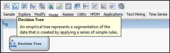
DecisionTree Node

The decision tree node is used for the decision tree model and is associated with the Model tab in SAS Enterprise Miner.

Figure 7.2: DecisionTree Node

Decision Tree Model Description

Decision Trees are a flexible model capable of handling various input and target data types, along with missing and non-standardized data. Decision trees can handle binary, continuous, or nominal inputs and output variables, whereas most models have more specific variable type requirements. Decision trees also do not require the statistical assumptions that must be met with models such as multiple linear regression. As a result, decision trees are one of the most popular and widely used techniques because they can also be easily communicated. Decision trees are modeled after actual trees, although in contrast with living trees, decision trees are often depicted top to bottom or left to right. Just like real trees, decision trees are grown starting with the primary node or trunk of the tree and following a series of branches, segments (or splits) based on the variables in the data set. The decision tree is fully grown following a series of splits (or branches) to the terminal nodes or leaves of the tree (Klimberg and McCullough, 2013).

Model Assumptions and Data Preparation

Due to the overall flexibility, decision trees carry fewer model assumptions and requirements than earlier models such as regression. However, decision trees, like regression, might suffer from overfitting the model, because the model is perfected for training data and has become unable to model new data. To avoid overfitting, we should again select the parsimonious model or simplest-best model. An advantage of the decision tree is that limited data preparation is required as compared with other models. Decision trees handle missing data and outliers to a greater extent and are less affected than other methods. Although data quality is always important, often time constraints impact model selection.

Partitioning Requirements

For decision trees, we typically create two data sets: 1. Training and 2. Validation. In some cases, three data sets might be used: 1. Training, 2. Validation and 3. Test. When using the third data set for the decision tree process, train the tree (or grow the tree to its full potential), and then validate (or prune) the tree to remove extemporaneous or invaluable branches and paths to simplify or improve the shape of the tree. Then, test the tree using the pruned model from validation.

Model Results Evaluation

To evaluate the results of our decision tree, we can use several items including errors, lift, misclassification rate, and English rules.

Errors

Errors are calculated from the predicted value less the actual value, which is also known as the residuals. Common measures of errors are sum of squared errors (SSE) and root mean square error (RMSE). The measures are calculated by taking the square or square root of the errors.

Lift

Lift is a measurement between a random or baseline model against the analytical model. A higher lift or outperformance of the random selection is best.

Misclassification Rate

For models with nominal or binary targets, the percentage of total records is misclassified as false positive or false negative.

English Rules

For decision trees, a tree model is available that can produce a set of IF…THEN conditions, which are also known as English rules, and they assist with the interpretability of the model. The rules are often used in decision support systems to model human decision-making. If you visit your physician, based on their experience, they will instinctively walk through a set of IF…THEN rules to make a diagnosis. For example, if you have a fever and cough, and stuffy nose, then you are diagnosed with influenza (or the flu).  

Now that we have covered the decision tree model, let’s continue with an experiential learning application to connect your knowledge of decision trees with a health application on patient mortality indicators.

Many quality improvement approaches to improve quality of care are based on manual activities without a direct link to the data within the healthcare information system, which can influence quality of treatment and cost of care. Payer and provider systems can supply patient outcome information and clinical pathways to support patient care. Data mining through decision trees allows for knowledge discovery from large sets of data that can be used to identify patterns or rules (Woodside, 2010b).

A decision tree can be used to determine how inpatient mortality rates compare to overall proportions, and which segments to focus on. In one study, a set of 8,405 patients were used for indicators of inpatient mortality as part of decision tree analysis to determine inpatient mortality factors. Factors and indicators included gender, discharge location (such as surgery department), age group, and disease class. The results found that for patients discharged from Internal medicine departments, mortality was nearly three times more likely than for other discharge locations. Patients with length of stay (LOS) over 16 days, resulted in a six times higher mortality rate. The variable significance included LOS and discharge department, followed by age group. Although logistic regression could be used, the output would be missing the segment characteristics that would be useful (Chae et al., 2003).

Previous studies have examined factors (such as gender, discharge department, age group, and disease class) to determine a relationship with mortality. For this experiential learning application, we want to verify which of these factors might have a relationship with mortality. To start our process, we first want to identify our input and target variables. In this application, our inputs (x) are gender, discharge location, age group, and disease class. Our target (y) is patient mortality. With a decision tree, one advantage is that the model can handle varying input and target variable types. In this application, our inputs are nominal, and our target variable is binary.

Data Set File: 7_EL1_Patient_Mortality.xlsx

Variables:

●       ID, unique identifier

●       Gender, (Female, Male)

●       Discharge Department, (Internal Medicine, Surgery)

●       Age, (Under 20, 21-40, 41-60, 61 or older)

●       Disease Class, (Circulatory, Congenital, Eye and Ear, Gastrointestinal, Miscellaneous, Muscle, Neoplasm, Pulmonary, Urinary)

●       Length of Stay, (1-5 Days, LOS 17-341 Days, LOS 6-16 Days)

●       Inpatient Mortality, (1=True, 0=False)

Step 1: Sign in to SAS Solutions OnDemand.

Step 2. Open SAS Enterprise Miner (Click SAS Enterprise Miner link).

Step 3. Create a New Enterprise Miner Project (Click New Project).

Step 4: Use the default SAS Server, and click Next.

Step 5: Add Project Name PatientMortalityIndicators, and click Next.

Step 6: SAS will automatically select your user folder directory (If using the desktop version, choose your folder directory), and click Next.

Step 7: Create a new diagram PatientMortalityIndicators (Right-click Diagram).

Step 8: Add a File Import node (Click the Sample tab, and drag the node onto the diagram workspace).

Step 9: Click the File Import node, and review the property panel on the bottom left of the screen.

Step 10: Click Import File and navigate to the 7_EL_1_Patient_Mortality.xlsx Excel File.

Step 11: Click Preview to ensure that the data set was selected successfully, and click OK.

Step 12: Right-click the File Import node, and click Edit Variables.

Step 13: Set Inpatient_Mortality to the Target variable role, set ID to the ID role, and all other variables to the Input role. Set the remaining variables according to their nominal, interval, or binary levels. To review an individual variable and to verify its role and level assignment, click the variable name and click Explore. You have finished setting all variables, click OK.

Figure 7.3: Edit Variables

 

Step 14: Add a Stat Explore node, Graph Explore node, and MultiPlot node (click the Explore tab, and drag the nodes onto the diagram workspace). Set the Graph Explore Property Sample Size to Max.

Figure 7.4: StatExplore and Graph Explore Nodes

 

 

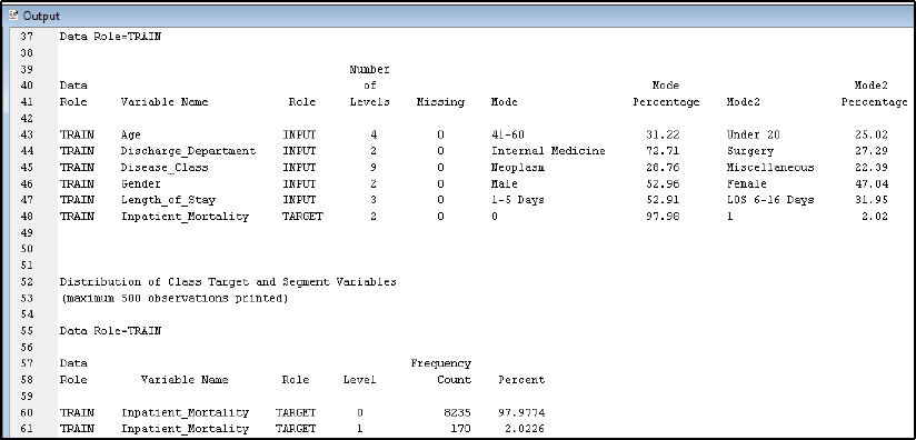
Step 15: Review the results. From the Stat Explore descriptive statistics results, we identify a good data quality result, which is verified through 0 missing records across variables. The breakout of the target variable Inpatient_Mortality is shown with 8235 records with a value of 0 (or False), and 170 records with 1 (or True).

Figure 7.5: StatExplore Results

 

 

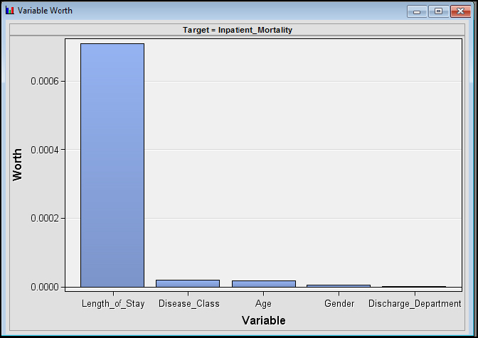
Step 16: Review the results. From the Stat Explore Variable Worth results, Length_of_Stay has the greatest variable worth with regard to our target variable of Inpatient_Mortality

Figure 7.6: StatExplore Results Variable Worth

 

 

Step 17: Review the results. From the Graph Explore results, we also see the breakdown of the Inpatient_Mortality.

Figure 7.7: Graph Explore Results

 

 

Step 18: Review the results. From the MultiPlot results, review each of the variables. For example, Age by Inpatient_Mortality shows a distribution across all age groups with both 0 and 1 frequencies.

Figure 7.8: MultiPlot Results

 

 

Step 19: From our Stat Explore, Graph Explore, and MultiPlot results, we see that the inpatient mortality is a rare event in terms of occurring only 2% in our data set. As a result, we will include a sampling node to conduct a rare event sampling to improve the final results. From the Sample tab, add a Sample node to the diagram and connect to File Import.

Figure 7.9: Add Sample Node

 

 

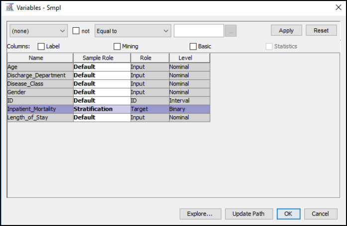
Step 20: Click the Sample node, and click the properties section. Then click Variables and set the Inpatient_Mortality to the Stratification Sample Role. The setting will allow us to select a sample based on the Inpatient_Mortality variable. Click OK.

Figure 7.10: Sample Properties Stratification

 

 

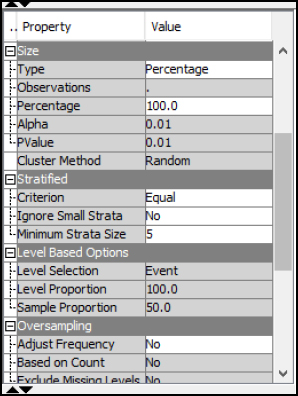
Step 21: Click the Sample node properties, and set the Type to Percentage and set the Percentage to 100. For the Stratified property, set the Criterion to Equal. The settings will select an equal sample of the Inpatient_Mortality rare event and the Inpatient_Mortality non-event. In other words, we will select an equal sample of both true and false cases of Inpatient_Mortality. If we selected the normal sample size, the results might be limited given the size of non-events, since all occurrences would favor a non-event scenario. Our goal is to find the factors leading to Inpatient_Mortality.

Figure 7.11: Sample Properties

 

 

Step 22: Run the Sample node and view the results. From the output, the original data set is shown with Inpatient_Mortality = 1/True occurring 170 times for 2% of the total data set. After sampling, Inpatient_Mortality = 1 occurs the same amount as Inpatient_Mortality = 0 for an equal sample data set.

Figure 7.12: Sample Results

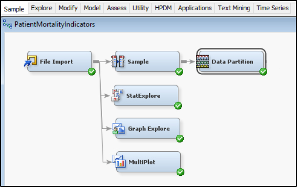
Step 23: Add a Data Partition node (Click the Sample tab, and drag the node onto the diagram workspace). Set the Data Partition Property Data Set Allocations to 60.0 for Training, 40.0 for Validation, and 0.0 for Test. Run the Data Partition node.

Figure 7.13: Data Partition Node

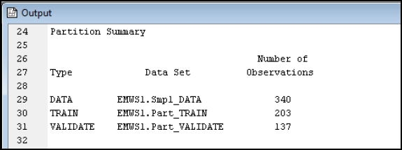
Step 24: Review the data Partition Results.

Figure 7.14: Data Partition Results

Step 25: Add an Impute node (Click the Modify tab, and drag the node onto the diagram workspace). Verify that the Impute Property is set to Count for Class variables and Mean for Interval variables.

Figure 7.15: Impute Node

 

 

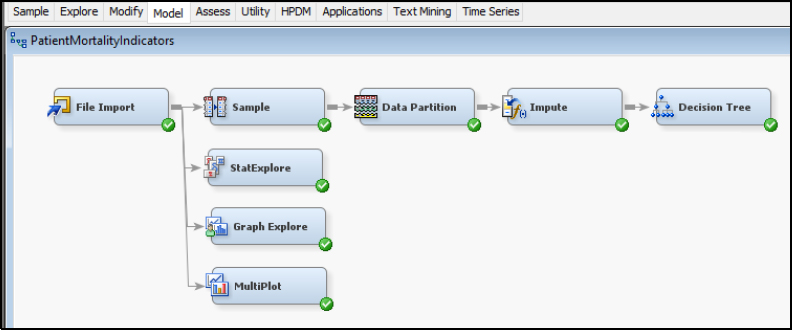
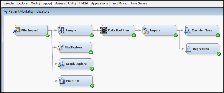
Step 26: Add a Decision Tree node (Click the Model tab, and drag the node onto the diagram workspace).

Figure 7.16: Decision Tree Node

Step 27: Select the Decision Tree node. In the Tree Property, under Splitting Rule, set Minimum Categorical Size to 2, and under Node, set Leaf Size to 1. The settings allow a tree to grow with a 2-category split and a single leaf or a single record.

Figure 7.17 Decision Tree Node Properties

 

 

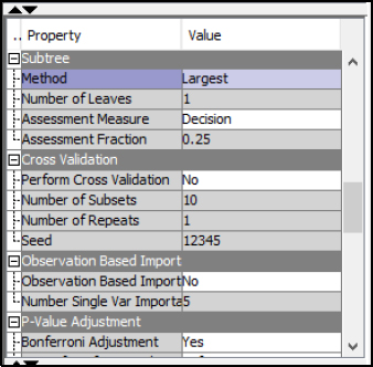
Step 28: Select the Decision Tree node. Under the Subtree property, select Largest. The property setting will run the full tree to all its branches and leaves, or all splits and decision points.

Figure 7.18: Decision Tree Node Properties

Step 29: Right-click the Decision Tree node, and click Run.

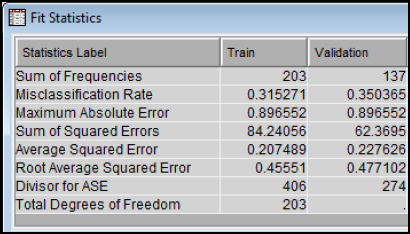
Step 30: Expand the Output Window Results and Review Model Results. The misclassification rate for the Training set is 31.5% and the Misclassification Rate for the Validation set is 35.0%.

Figure 7.19: Decision Tree Node Results

 

 

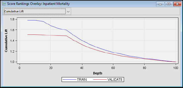
Step 31: Review the Model Results. The cumulative lift shows that the model outperforms a random model. At the top 10% of records (or depth), the train model outperforms a random model by nearly 1.8 times and the validation model by 1.5 times. 

Figure 7.20: Decision Tree Node Results

 

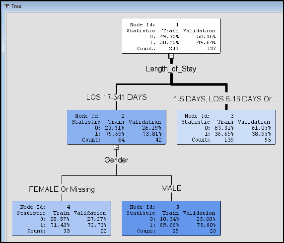
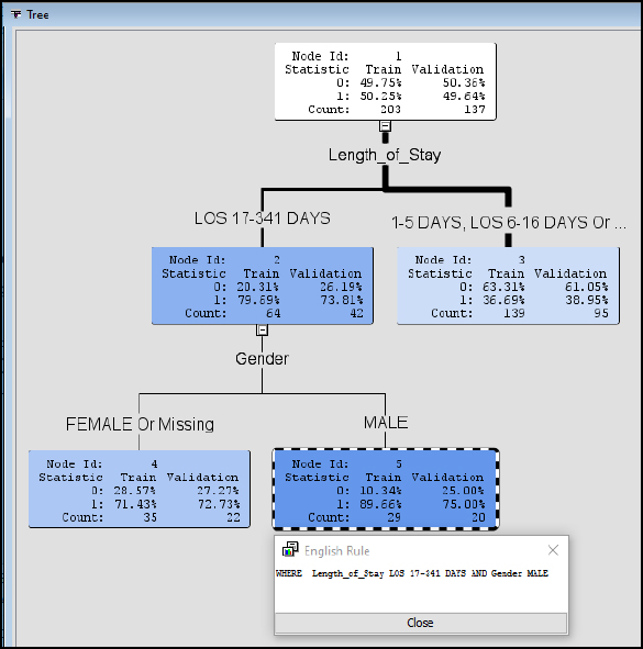
Step 32: Review the Model Results. The decision tree is presented as a visual model. Think of the decision tree as modeled after a living tree. At the top, we have the root or Node Id 1. The top is where the tree starts is like the trunk of a tree. Node Id 1 also gives a breakdown of our data with about 50% 0 and 50% 1 cases and a split between Train with 203 records and Validation with 137 records. The lines can be considered branches, and the remaining nodes are leaves. Therefore, we build (or grow) our tree starting with the root or Node Id 1 and branching out all the way to the final leaves Node Id 5. A final leaf is also known as a terminal node. The lines (or branches) are also different widths or thicknesses based on the number of records. Try to visualize an upside-down tree in the Figure 7.21 Starting again from the root Node Id 1, the first split in the tree occurs with the variable Length_of_Stay. This indicates that Length_of_Stay has a high variable importance in our model. If we follow the split to the left, we have LOS 17-341 Days, this means that all records with LOS 17-341 Days follow the left side of the split. The right side of the Length_of_Stay split contains all records with LOS 1-5 Days, 6-16 Days, or missing values. Looking closer at Node Id 2, you can see that the record breakdown is also given. For Validation, 26.19% are 0 cases and 73.81% are 1 cases. This indicates that using a LOS of 17-341 Days split, we can identify 80% of the 1 (or true) cases for patient mortality. We can further follow the tree to the next split and branches for Gender. Follow the tree to Gender of Male and Node Id 5. For the Validation breakdown, we find 75% are 1 cases and 25% are 0 cases, with true cases slightly higher for males than females.

Figure 7.21: Decision Tree Node Results

Step 33: Review the Model Results. We can further develop programmatic IF…THEN rules to describe the branches, which are also known as English Rules. The rules can be valuable for automating decision- making in a system such as a decision support or EHR system that used by medical professionals for assessing risk of morality and developing an appropriate plan of care. Click Node Id 5 and right-click and select Tools ▶ Display English rule. 

Figure 7.22: Decision Tree Display English Rule

 

Step 34: Review the Model Results. The results will display the English Rule following the tree structure, Where Length_of_Stay (LOS) is 17-341 AND Gender is MALE. The rules are easily communicated to other clinical and non-clinical individuals. For example, if the length of stay is between 17 and 341 days and the patient is male, nearly 90% of our training records and 75% of our validation records indicate patient mortality.

Figure 7.23: Display English Rule

 

Step 35: Add a Regression node. From the previous chapter, we can also include a Regression model for our data set. The node can be connected in a way that is similar to the Decision Tree node. Run the Regression node.

Figure 7.24: Regression Node

Step 36: Review the Model Results. The misclassification rate for the Training set is 29.1%, and the misclassification rate for the Validation set is 38.7%. The results perform similarly to our Decision Tree model, with 31.5% and 35% misclassification rate, respectively. 

Figure 7.25: Regression Node Fit Statistics

Step 37: Review the Model Results. Adding the Regression node also provides additional results such as Odds Ratio. From the Analysis of Maximum Likelihood Estimates output, the Length_of_Stay is a significant variable with Pr > ChiSq, p-value less than 0.01. From the odds ratios, the length of stay, 17-341 days, carries a 6.752 times the odds of mortality than a length of stay 6-16 days.

Figure 7.26: Regression Node Output

 

In summary, the decision tree will take the form of 1 or more inputs and 1 target variable. The inputs can be interval, binary, or nominal, and the target can also be interval, binary, or nominal. To evaluate the decision tree, we can use error, lift, English rules, and misclassification rate for a binary, nominal, or categorical target variable.

●       Model: Decision Tree node

●       Decision Tree: 1+ input and 1 target variable

●       Input: Interval, Binary, or Nominal

●       Target: Interval, Binary, or Nominal

●       Evaluation: Error, Lift, English Rules, Misclassification Rate

One study found that people often evaluate their overall health and wellness based on their lived health rather than their experience of biological health. The self-reported general health (SRGH), contains the levels of very good, good, fair, bad, and very bad. SRGH is one of the most commonly used measures of health in population health and clinical health surveys and is used to compare populations. Nearly 2,000 scientific studies have been conducted using SRGH (or general survey questions) about how you would rate your health. The question is also used internationally and is included as part of the European Organization of Research and Treatment of Cancer (EORTC) Quality of Life Questionnaire. SRGH has been used as an input variable for predicting health outcomes, such as mortality, or it is used as a target variable based on inputs such as diagnosis and symptoms (Bostan et al., 2014).

For the experiential learning application that you have been provided, a sample of 27,446 records with SRGH is the target variable, and setting type, gender, age group, education, number of health conditions, biological health score, and lived health score are the input variables. Help your management team answer the following question.

Question: Which factors might influence SRGH?

Data Set File: 7_EL2_SRGH.xlsx

Variables:

●       Population Type: 17,739 Community-Dwelling, 9,707 Institutionalized Population

●       SRGH: Very Good, Good, Fair, Bad, very bad

●       Gender (male, female)

●       Age groups (<=65,>65)

●       Education (no school, primary-school-incomplete, primary-school-complete, secondary school first step, secondary school finished, professional school medium, professional school superior, University)

●       Number of health conditions (0, 1-2, > 2). The health conditions were: Spinal cord injury, Parkinson’s, Lateral sclerosis, Multiple sclerosis, Agenesis/Amputation, Laryngectomy, Arthritis, Rheumatoid arthritis or Ankylosing spondylitis, Muscular dystrophy, Spina bifida/hydrocephaly, Myocardial infarction or Ischaemic cardiopathy, Cerebrovascular accidents, Down's Syndrome, Autism and other disorders associated with autism, Cerebral paralysis, Acquired brain damage, Senile Dementia of the Alzheimer Type, Other types of dementia, Schizophrenia, Depression, Bipolar disorder, Pigmentary retinosis, Myopia magna, Senile macular degeneration, Diabetic retinopathy, Glaucoma, Cataract, HIV/AIDS, Rare illnesses, Cancer (only for community dwelling population).

●       Biological Health Score 0 (best biological health) to 100 (worst biological health)

●       Lived Health Score 0 (best lived health) to 100 (worst lived health)

Follow the SEMMA process for your experiential learning application and provide recommendations. A template has been provided below that can be reused across future projects.

Title	Self-Reported General Health
Introduction	Provide a summary of the business problem or opportunity and the key objective(s) or goal(s). Create a new SAS Enterprise Miner project. Create a new Diagram.
Sample	Data (sources for exploration and model insights) Identify the variables data types, the input and target variable during exploration. Add a FILE IMPORT Provide a results overview following file import: Input / Target Variables Generate a DATA PARTITION
Exploration	Provide a results overview following data exploration Add a STAT EXPLORE Add a GRAPH EXPLORE Add a MULTIPLOT Summary statistics (average, standard deviation, min, max, and so on.) Descriptive Statistics Missing Data Outliers
Modify	Provide a results overview following modification Add an IMPUTE
Model	Discovery (prototype and test analytical models) Apply a decision tree model and provide a results overview following modeling. Add a DECISION TREE Model description Analytics steps Decision Tree results (tree model, English rules) Model results (Lift, Error, Misclassification Rate) Selection Model
Assess and Reflection	Provide overall recommendations to business Model advantages / disadvantages Performance evaluation Model recommendation Summary analytics recommendations Summary informatics recommendations Summary business recommendations Summary clinical recommendations Deployment (operationalization plan: timeline, resources, scope, phases, project plan) Value (return on investment, healthcare outcomes)

Review, reflect, and retrieve the following key chapter topics only from memory and add them to your learning journal. For each topic, list a one sentence description/definition. Connect these ideas to something you might already know from your experience, other coursework, or a current event. This follows our three-phase learning approach of 1) Capture, 2) Communicate, and 3) Connect. After completing, verify your results against your learning journal and update as needed..

Key Ideas – Capture	Key Terms – Communicate	Key Areas - Connect
Payer Anamatics
Payers
Claims System and Process
Claims Forms
EDI
Claims Adjudication
Decision Tree
Inpatient Mortality Application
Self-Reported General Health