
Chapter 5
Filtering and Transformations
Wolfgang Birkfellner
5.1 The Filtering Operation
A filter in mathematics or signal processing describes a function that modifies an incoming signal. Since images are two- or three dimensional signals, a filter operation can, for instance, remove noise or enhance the contrast of the image. In this chapter, we will learn about some basic filtering operations, the basics of signal processing, and we will encounter a powerful tool in signal processing.
In order to get a systematic overview of filtering operations, a completely non-medical example might prove useful. We know that a convex lens, made of a material that changes the speed of light, can focus incoming light. Crown glass, with a refractive index n = 1.51, is the most common material for lenses. The focusing of incoming rays of light (which are the normals to the wavefront) is achieved by the fact that at least one boundary layer between air and glass is curved. The rays that intersect the lens surface on the outer diameter have a shorter travel through the glass, whereas the ray that intersects the middle of the lens (the so-called paraxial ray) has to stay within the glass for a longer period of time. Since the speed of light changes in the optically dense medium, the paraxial ray lags behind his neighbors, and as a consequence, the rays (which are, again, normals to the wavefront) merge in the focus. The angle of the ray is determined by the law of refraction.1
A mirror can also focus light; here, the more simple law of reflection governs the formation of the focus. Each incoming ray is reflected by an angle of the same absolute value as the angle of incidence. In a spherical mirror (which bears its name because it is part of a sphere), all rays emerging from the center of curvature (COC) are reflected back to the COC; in this case, the COC is the focus of the mirror. When rays come from a different position than the COC, the reflected rays are no longer focused in a single spot – rather than that, the rays close to the paraxial ray have a different focus than the rays which hit the mirrors edge. Figure 5.1 illustrates this behavior, which is called spherical aberration. The consequences are clear; if we mount an image detector such as a CCD, we will not get a sharp image since the rays emerging from a point-shaped object (such as, star) are not focused to a single spot. A spherical mirror is therefore not a very good telescope.

An illustration of the spherical aberration in a mirror. If a single point source of light is located at the center of curvature (COC), all rays of light will be reflected back to the COC, which is also the location of the focus in this case. This situation is illustrated in the left part of the image. If the point source is located at infinity, all rays come in parallel; in this case, the rays closer to the center of the mirror form a different focus than the distal rays. In other words, the light from the point source is not focused to a single spot – the image will be unsharp.
We can model this optical aberration using a so-called ray tracing program. It is already apparent that these programs for the design of optical systems do something similar to the rendering algorithm we will encounter in Chapter 8. One of these raytracing programs is OSLO (Sinclair Optics, Pittsford, NY), which we will use to model the extent of the spherical aberration in a spherical mirror of 150 mm diameter and a focal length of 600 mm. The task in optical design is to optimize the parameters of the optical elements in such a manner that the optical systems deliver optimum image quality. This is achieved by simulating the paths of light rays through the optical system. The laws of reflection and refraction are being taken into account. The optical system is considered optimal when it focuses all possible rays of light to a focus as small as possible. OSLO computes a spot diagram, which is a slice of the ray cone at its minimal diameter; the spot diagram therefore gives us an idea of what the image of the point source of light will look like after it passes the spherical mirror. We assume a single monochromatic point source of light at infinity. The resulting spot diagram can be found in Figure 5.2.

The spot diagram of a spherical mirror of 150 mm diameter and 600 mm focal length. OSLO simulates a point light source located at infinity here. As we can see, the smallest image possible of this point source on an image detector is a blob of approximately 1 mm diameter. The spot diagram is a representation of the point-spread function, which is the general concept of modelling signal transfer by an arbitrary signal processing system.
Here ends our excursion into optics; the mirror is, in fact, a filter - it modifies the original signal to something else. If we want a perfect telescope (or another imaging system), we should take care that the image provided is as identical as possible to the original. The way to describe the performance of such a signal transferring system is actually the performance on a single, point like source. The result of the filter on this point-like signal is called the Point Spread Function (PSF). If we want to know about the looks of the whole image, we simply have to apply the PSF to every single point in the original image. The process of blending the PSF with the original image is called convolution. In the convolution operation, the PSF is applied to every pixel, which of course might also affect the surrounding pixels in the resulting image. The convolution operation is denoted using the * sign. Many textbooks in image processing introduce the various image processing operations by providing small matrices, which represent a convolution kernel. Subsequently, this kernel, which can be considered a PSF, is applied to every single pixel and re-distributes the gray values ρ in order to achieve the desired outcome. In this course, we will try to avoid this formulation in favor of a more strict (and simple) formalism for convolution, which will be introduced in Section 5.2.2.
5.1.1 Kernel based smoothing and sharpening operations
A common task in image processing is the smoothing and sharpening of images; an image corrupted by noise - which can be considered ripples in the landscape of gray values ρ - may be improved if one applies an operation that averages the local surrounding of each pixel. Such a kernel K can, for instance, take the following form:
Kblur=110(111121111) (5.1).
So what happens if this kernel is convolved with an image? In fact, a weighted average of the gray values surrounding each pixel in the original images is assigned to the same pixel position in the new image. Small fluctuations in the gray values are reduced by this averaging operation. However, the central pixel position is emphasized by receiving a higher weight than the others. Example 5.4.1 illustrates this simple operation; a detail of the outcome is also given in Figure 5.3. In data analysis, this is referred to as a moving average. Another interesting detail of this kernel is also the fact that it is normalized by multiplying every component of Kblur with the factor 110. It is clear that a blurring PSF like Kblur, which essentially does something similar to the spherical mirror, cannot add energy to a signal -and therefore, the total sum of elements in the kernel is one. It is of the utmost importance to emphasize that kernels such as the blurring kernel given in Equation 5.1 are indeed functions, just like the images they are convolved with.
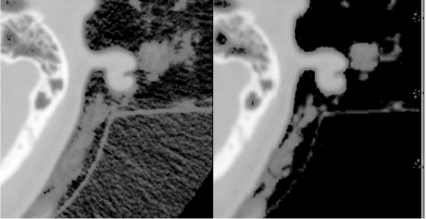
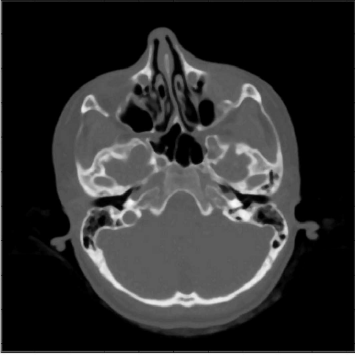
A detail from the SKULLBASE.DCM before and after the smoothing operation carried out in Example 5.4.1. The whole image (a CT slice in the vicinity of the skull base) is shown in Figure 5.24. On the left side, we see some reconstruction artifacts in the air surrounding the head. The smoothing filter Kblur successfully removes these artifacts by weighted averaging. For visualization purposes, the image intensities were transformed here in order to improve the visibility of low contrast details. Image data courtesy of the Dept. of Radiology, Medical University Vienna.
Let’s go back to the spherical telescope. A star emits energy; a small fraction of this energy hits the mirror, which focuses this energy onto an image detector. Due to spherical aberration, the image is blurred, therefore the energy is distributed over more than one pixel of our image detector. As we may recall from Chapter 4, the gray value is proportional to the energy as long as we stay within the dynamic range of the detector. There is no obvious reason why the telescope should add energy to the signal. Kblur should not do so, either. If a kernel changes the sum of all gray values ρ, one might consider normalizing the whole image by a simple global intensity scaling to the same value Σi,j ρi,j found in the original image.
The opposite of smoothing is an operation called sharpening; in a sharpening operation, it is desired to emphasize edges in the images. Edges can be considered an abyss in the landscape of the image. A sharpening operator therefore does merely nothing if the surrounding of a pixel shows a homogeneous distribution of gray values. If a strong variation in gray values is encountered, it emphasizes the pixels with high intensity and suppresses the low intensity pixels. The classic sharpening operator looks like this:
Ksharp=(−1−1−1−19−1−1−1−1) (5.2)
It strongly weights the pixel it operates on, and suppresses the surrounding. The region from SKULLBASE.DCM from Figure 5.3 after applying Ksharp is shown in Figure 5.4. An interesting effect from applying such a kernel can, however, be observed in Example 5.4.1; the strong weight on the central pixel of Ksharp causes a considerable change in the shape of the histogram. Still, Ksharp preserves the energy stored in a pixel. The change in image brightness is a consequence of the scaling to 6 bit image depth - check Example 5.4.1 for further detail.

The same detail from the SKULLBASE.DCM already shown in Figure 5.3 after a sharpening operation using the Ksharp kernel. Fine details such as the spongeous bone of the mastoid process are emphasized. Image data courtesy of the Dept. of Radiology, Medical University Vienna.
Both smoothing and sharpening operations are widely used in medical imaging. A smoothing operator can suppress image noise, as can be seen from Figure 5.3. In modalities with a poor SNR, for instance in nuclear medicine, this is quite common. Sharpening, on the other hand, is a necessity in computed tomography to enhance the visibility of fine detail, as we will see in Chapter 10. Figure 5.5 shows two CT slices of a pig jaw; one is not filtered after reconstruction, the other one was filtered using the software of the CT. Besides the improvement in detail visibility and the increased visibility of reconstruction artifacts, we also witness a change in overall image brightness - a phenomenon we have already seen in Figure 5.4. It is also an intensity scaling artifact.

Two CT slices of a dry mandible of a pig. The left image was reconstructed without the use of a sharpening operator, the right slice was sharpened. Both images were directly taken from the DICOM-server connected to the CT and not further processed. Again, the change in overall image brightness from the use of the sharpening operator is clearly visible. This is, however, an intensity scaling artifact. Image data courtesy of the Dental School Vienna, Medical University Vienna.
A large number of other kernels can be defined, and they usually just represent different types of PSFs. Kblur, for instance, is a simple numerical approximation of a two-dimensional Gaussian curve. In numerical mathematics, we have already seen that functions are simply represented as vectors of discrete values, which represent the result of a function (see, for instance, Example 4.5.4). If we want to use more precise kernels, we may simply increase the number of pivoting values. For instance, a more sophisticated Gaussian kernel with five instead of three pivoting elements in each dimension looks like this:
K5×5gauss=1256(1464141624164624362464162416414641) (5.3)
The single elements of the kernel K5×5 Gauss are approximated from the well known analytic expression for the Gaussian curve. However, the more precise a kernel gets, the more time consuming the actual implementation is.2 As already announced in the introduction to this chapter, a more convenient formalism for convolution with complex kernel functions exists, therefore we will now close this section.
5.1.2 Differentiation and edge detection
Since images can be considered mathematical functions, one can of course compute derivatives of these images. We know that the derivative of a function gives a local gradient of the function. However, the problem in image processing lies in the fact that we cannot make assumptions about the mathematical properties of the image such as differentiability. The good news is that we can make numerical approximations of the derivation process. The differential expression df(x)dx for a function f(x) = ρ becomes a finite difference:
df(x)dx=ρi+1−ρiΔx (5.4)
In this special case, we are dealing with a forward difference since the numerator of the differential is defined as the difference between the actual value ρi and its next neighbor ρi+1. There is also a backward difference and a central difference, which we will encounter in the next sections. In Example 5.4.3, we will apply this operation to a simple rectangular function; the result can be found in Figure 5.6.
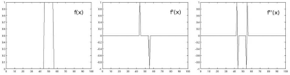
The results from Example 5.4.3. In the first plot, we see a simple rectangle function f(x). The first derivative df(x)dx, computed by forward differentiation, is named f′(x) in this illustration. As we can see, the derivative takes a high value if something rapidly changes in f(x), and it becomes zero if neighboring values of f(x) are similar. The same holds true for the second derivative f″(x). In image processing, differentiation yields the edges of an image, whereas areas of similar gray values become black.
A function that maps from two or three coordinates to a scalar value (such as an image) features a derivative in each direction - these are the partial derivatives, denoted as ∂I(x,y,z)∂x, ∂I(x,y,z)∂y and so on if our function is the well known functional formulation I(x,y,z) = ρ as presented in Chapter 3. The forward difference as presented in Equation 5.4, again, is the equivalent of the partial derivative: ∂I(x,y,z)∂x=ρx+1,y,z−ρx,y,z, where ρx,y,z is the gray value at voxel position (x,y,z)T; the denominator Δx is one, and therefore, it is already omitted. If we want to differentiate an image, we can define a kernel that produces the forward difference after convolution with the image. Such a kernel for differentiation in the x-direction is given as:
Kx-forward=(0000−11000) (5.5)
The correspondence between Kx-forward and Equation 5.4 is obvious. The kernel subtracts the gray value ρx,y located at the central pixel from the gray value ρx+1,y located to the right. Kx-forward therefore computes the partial forward difference of an image Ix,y. The effects of Kx-forward are also presented in Example 5.4.3. The result of applying forward differentiation on the already well-known SKULLBASE.DCM image is shown in Figure 5.7. Apparently, all the homogeneous gray value information is lost, and only the edges in the image remain. Due to the forward differentiation, the whole image shows some drift to the right hand side. Kx-forward is also known as the bas-relief kernel; SKULLBASE.DCM looks a little bit like a lunar landscape since it shows shadows in the positive x-direction, and the whole image is also pretty flat. While Kx-forward is an edge-detection filter in its simplest form, the dullness of the whole image is somewhat disturbing. The cause of this low contrast can be guessed from the middle image showing the first derivative of the rectangle function in Figure 5.6 - when proceeding from a low value of f(x) to a high value, the derivative takes a high positive value; if f(x) is high and f(x + 1) is low, the derivative yields a high negative value. However, when detecting edges, we are only interested in the sudden change in image brightness - we are not interested in the direction of the change. A modification of Kx-forward is the use of the absolute value of the gradient. This is an additional task for you in Example 5.4.3, and the result is found in the right image in Figure 5.7.
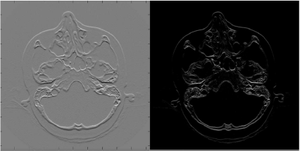
Some more results from Example 5.4.3. The left image shows the effects of Kx-forward on the SKULLBASE.DCM-image. It is pretty evident why this filter is also called the bas-relief filter. When computing the absolute value of the convolution of Kx-forward with SKULLBASE.DCM, the image on the right is produced. It does always give a positive value, no matter whether the image edges change from bright to dark pixel values or vice versa. In can also be seen that vertical edges like the skin surface close to the zygomatic arch is not emphasized; the x- and y-axis are swapped - this is a direct consequence of the matrix indexing conventions in MATLAB, where the first index is the column of the matrix image. Image data courtesy of the Dept. of Radiology Medical University Vienna.
Given the rather trivial structure of Kx-forward, the result of this operation as presented in Figure 5.7 is not that bad for a first try on an edge detection filter. Only two problems remain. First, only the partial derivative for the x-direction is computed, whereas the y-direction is neglected. And the forward-direction of Kx-forward gives the image a visual effect that simulates a flat relief. Both issues can easily be resolved.
If we want to know about the gradient - the direction of maximal change in our image I(x,y,z) = ρ - we have to compute all partial derivatives for the independent variables x, y, and z, and multiply the result with the unit vectors for each direction. Mathematically speaking, this is the nabla operator ∇=(∂∂x,∂∂y,∂∂z)T; it returns the gradient of a function as a vector. Computing the norm of the nabla operator and I(x, y, z) gives the absolute value of the maximal change in the gray scale ρ.
||∇I(x,y,z)||=√(∂I(x,y,z)∂x)2+(∂I(x,y,z)∂y)2+(∂I(x,y,z)∂z)2 (5.6)
What looks mathematical and strict is in fact very simple; it is the length of the gradient. The fact that this gradient length is always positive also makes the use of the absolute value of a differentiation kernel as proposed for Kx-forward unnecessary. The asymmetric nature of the forward differentiation from Equation 5.4 can be replaced by the average of the forward-and the backward difference. This so-called central difference is given by
df(x)dx=12(ρi+1−ρi︸ForwardΔ+ρi−ρi−1︸BackwardΔ) (5.7)
for a stepwidth of Δx = 1. This expression can be rewritten as df(x)dx=12(ρi+1−ρi−1). This central difference yields the following 2D convolution kernels for derivations in × and y
Kx-central=12(000−101000)andKy-central=12(0−10000010) (5.8)
Therefore, the result of the operation
√(Kx-central*I(x,y))2+(Ky-central*I(x,y))2,
which is actually the length of the gradient of the image I(x,y) should give a rather good edge detection filter. In Example 5.4.3, you are prompted to implement that operation.
The Kx-central and Ky-central kernels obviously provide a nice edge detection filter, as we can see from Figure 5.8. We can, of course, widen the focus of the kernels. For instance, it is possible to add more image elements to the kernel, as we have seen in Equation 5.3, where our simple smoothing kernel Kblur was enhanced by modelling a Gaussian curve over a 5 × 5 kernel. The general concept of connectedness can be introduced here; a pixel has four next neighbors - these are the four-connected pixels. Beyond that, there are also the eight-connected neighbors. If we add the contributions of the next but one neighbors to the center of the kernel, we are using the eight-connected pixels as well. Kx-central and Ky-central only utilize the four-connected neighbors, whereas Ksharp and Kblur are eight-connected. Figure 5.9 gives an illustration. From this illustration it also evident that the neighbors on the corners of the kernel are located at a distance √2Δx from the center of the kernel with Δx being the pixel spacing. Therefore the weight of these image elements that are distant neighbors is lower. The concept of connectedness can of course be generalized to 3D. The equivalent to a four connected neighborhood is a six connected kernel (which also uses the voxel in front of and behind the central voxel), and if we also use the next but one voxels to construct our kernel, we end up with 26 connected voxels.
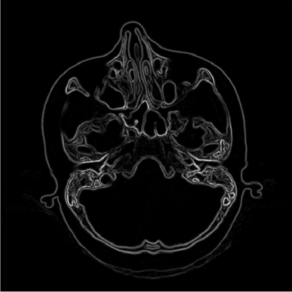
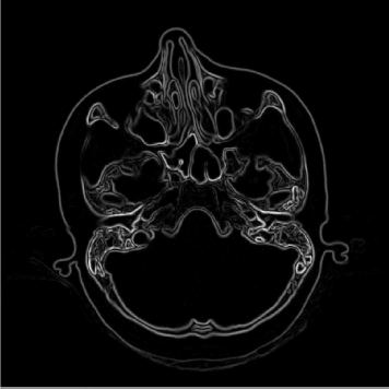
The effects of computing the length of the resulting gradient after convolution result of Kx-central and Ky-central with SKULLBASE.DCM. This is already a pretty satisfying edge detector; due to the use of central differences, no shadowing effects appear. The use of the total differential does respect changes in all directions, and the gradient length only yields positive results for the derivation result. Image data courtesy of the Dept. of Radiology, Medical University Vienna.

The four-connected and eight-connected neighborhood of a pixel. The contribution from the neighboring pixels depends on their distance; the pixels on the corner are at a distance that is larger by a factor √2 compared to the 4-connected neighbors. If a kernel utilizes information from these next but one neighbors, there has to be assigned a lower weight than to the nearest neighbors.
A more general formulation of the kernels from Equation 5.8 including the next and next but one neighboring pixels (while omitting the factor 12) and assigning appropriate weights (rounded down to integer numbers) to the next and next but one pixels would be:
KSobelx=(−101−102−101)andKSobely=(−1−2−1000121) (5.9)
As the subscript already shows, these are the Sobel-kernels, which are among the best known edge detection operators in image processing.
Many more kernels can be designed, and many of them are virtually redundant and can be constructed as linear combinations of the kernels presented. However, blurring, sharpening, and edge detection are among the most common and important operations in medical imaging. What all kernels presented until now have in common is the fact that they are linear; the kernel can be applied to the whole image, or one can divide the kernel in parts and apply the filter subsequently to the image. After fusing the outcome, the result is the same. If an image I(x,y) = I1(x, y) + s*I2(x,y) is convolved with an arbitrary linear kernel K, the following identity is true:
K*I(x,y)=K*I1(x,y)+s*K*I2(x,y) (5.10)
Another similarity of all the kernels presented so far is the fact that they are constant; the weights in the kernel are always the same, no matter what gray value ρ is encountered by the central pixel of the kernel. A somewhat adaptive technique that bears its name from analog photography is unsharp masking. Originally designed to cope with the limited dynamic range of photographic paper, the analog unsharp masking operation consists of exposing a photographic plate with a defocused image from negative film. If the plate has the same size as the photographic paper, one can expose the focused image of the negative through the developed photographic plate onto photographic paper. Both a sharpening effect and a suppression of overexposed areas is the result; while dynamic range is no longer that big an issue in digital imaging, the sharpening effect is still widely used, and the procedure from analog photography - exposition of the unsharp mask and summation of the unsharp mask and the focused image - can directly be transferred to the world of digital image processing.
First, we need the unsharp mask, which can be derived using blurring kernels such as K5×5 Gauss or Kblur; subsequently, the unsharp mask is subtracted from the original image. Therefore, an unsharp masking kernel KUnsharp Mask using the simple smoothing filter Kblur looks like this:
KUnsharp Mask=(000010000)︸Unity operator−ω*Kblur (5.11)
The unity operator is the most trivial kernel of all; it simply copies the image. Example 5.4.4 implements this operation. ω is a scalar factor that governs the influence of the low pass filtered image on the resulting image. Denote that the convolution operation by itself is also linear: K1 * I(x,y) + s * K2 * I(x,y) = (K1 + s * K2) * I(x,y). We can therefore generate all kinds of kernels by linear combination of more simple kernels.
5.1.3 Helpful non-linear filters
While most filters are linear and fulfill Equation 5.10, there are also non-linear filters. The most helpful one is the median filter. The median of a set of random variables is defined as the central value in an ordered list of these variables. The ordered list of values is also referred to as the rank list. Let’s take a look at a list of values xi for an arbitrary random variable, for instance xi ∈ 5,9,12,1,6,4,8,0,7,9,20,666. The mean of these values is defined as ˉx=1N∑ixi, where N is the number of values. In our example, ˉx is 62.25. This is not a very good expectation value since most values for xi are smaller. However, we have an outlier here; all values but the last one are smaller than 21, but the last value for xi screws everything up. The median behaves differently. The rank list in our example would look like this: xi ∈ 0,1,4,5,6,7,8,9,9,12,20,666. Since we have twelve entries here, the central value lies between entry #6 and #7. The median of xi is 7.5 - the average of the values x6 and x7 in the ordered rank list. The strength of the median is its robustness against outliers. As you can see, the median differs strongly from the average value ˉx. But it is also a better expectation value for x. If we pick a random value of xi, it is more likely to get a result close to the median than a result that resembles ˉx.
A median filter in image processing does something similar to a smoothing operation - it replaces a gray value ρ at a pixel location (x, y)T with an expectation value for the surrounding. It is remarkable that the median filter, however, does not change pixel intensities in an image - it just replaces some of them. As opposed to Kblur and K5×5 Gauss, it does not compute a local average, but it uses the median of a defined surrounding. In general, the median filter for 3D and a kernel of dimension n × m × o is defined in the following way:
Record all gray values ρ for the image elements in a surrounding of dimension n×m×o.
Sort this array of gray values.
Compute the median as the one gray value located in the middle of the sorted vector of gray values.
Replace the original pixel by this median.
Example 5.4.5 gives an implementation of a 5 × 5 median filter. Compared to linear smoothing operators, the median filter retains the structure of the image content to a larger extent by preserving image edges while being very effective in noise suppression. A comparison of smoothing and median filters of varying kernel size is given in Figure 5.10. The power of the median filter is demonstrated best when taking a look at “salt and pepper” noise, that is images stricken with black or white pixels, for instance because of defective pixels on the image detector. A median filter removes such outliers, whereas a simple blurring operation cannot cope with this type of noise.

A topogram of a mouse from MicroCT with 733 × 733 pixels. The upper row shows the effects of low-pass filtering with varying kernel sizes. For comparison, the same image underwent median filtering with similar kernel sizes, which is shown in the lower row of images. While the median filter is a low-pass filter as well, the visual outcome is definitively different. The images can also be found on the CD accompanying this book in the JPGs folder. Image data courtesy of C. Kuntner, AIT Seibersdorf, Austria.
Not all non-linear filters are based on sorting or selection processes; an interesting filter that yields similar results compared to the median filter as a smoothing filter that retains general image structure is the anisotropic diffusion filter, which will be introduced as an example for a whole class of iterative filters. Imagine a glass of water with an oil layer covering it. If you release a drop of ink in the water layer, the ink will slowly diffuse within the water layer, but not the oil layer. Over time we will see nothing but a slightly tinted water layer. This process, which is based on the Brownian motion of the water molecules, is called diffusion. Mathematically, it is described by a partial differential equation (PDE). While the PDE itself is always the same for all possible substances, the outcome is governed by various parameters such as the viscosity of the fluid, the concentration of the substances and so on. The PDE can be solved numerically. If we consider an image to be a distribution of different substances, with ρ being a measure of the concentration, we can define a filter that simulates the diffusion of the image intensities over time. The various boundary conditions and the number of time steps chosen allow for a very fine tuning of the filter. In fact, the anisotropic diffusion filter is a very powerful tool for noise suppression. The effects of the filter are shown in Figure 5.11, which was generated using the AnalyzeAVW 9.1 software (Biomedical Imaging Resource, Mayo Clinic, Rochester/MN).
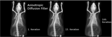
The same topogram as in Figure 5.10 after anisotropic diffusion filtering. As the diffusion process proceeds (as indicated by the number of iterations), one can see how the images get more blurred; still, structure is largely retained. The anisotropic diffusion filter is another example for a non-linear lowpass filter. Here, the large number of parameters allow for a very fine tuning of the degree of blurring and noise reduction. Image data courtesy of C. Kuntner, AIT Seibersdorf, Austria.
5.2 The Fourier Transform
5.2.1 Basic linear algebra and series expansions
Throughout this book, we tried to make the mathematics of medical image processing as tangible as possible. Therefore we restrict ourselves to a few equations and rely on the illustrative power of applied programming examples. Now, we will proceed to a chapter that is of immense importance for signal processing in general; however, it is also considered sometimes to be difficult to understand. We are now talking about the Fourier transform, which is based on the probably most important orthonormal functional system. And it is not difficult to understand, although the introduction given here serves only as a motivation, explanation, and reminder. It cannot replace a solid background in applied mathematics.
We all know the representation of a vector in a Cartesian coordinate system3: →x=(x1,x2)T. That representation is actually a shorthand notation. It only gives the components of the vector in a Cartesian coordinate system, where the coordinate axes are spanned by unit vectors →ex=(1,0)T and →ey=(0,1)T. The vector →x is therefore given by the sum of unit vectors, multiplied with their components x1 and x2: →x=x1→ex+x2→ey. Figure 5.12 shows a simple illustration. We can invert this formulation by using the inner product (also referred to as scalar product or dot product). The inner product of two arbitrary 3D vectors →y=(y1,y2,y3)T and →z=(z1,z2,z3)T is defined as:
→y•→z=(y1y2y3)•(z1z2z3)=y1z1+y2z2+y3z3=||→y||||→z||cos (α) (5.12)
α is the angle enclosed by the two vectors →y and →z, and the ||...|| operator is the norm of the vector - in this case, the vector’s length. A geometrical interpretation of the inner product in three dimensional space is the projection of one vector onto the other times the length of both - see the last equality in Equation 5.12 . However, one has to be aware that Equation 5.12 is only valid if the coordinate system is orthonormal - all unit vectors have to be orthogonal to each other and their length has to be 1. Mathematically speaking, it is required that the inner product of two unit vectors →ei and →ej is one if i equals j and zero otherwise:
→ei•→ej=δij (5.13)
δij is the so-called Kronecker-function, defined as
δij={1 ifi=j0 ifi≠j (5.14).

The representation of a vector →x=(1,2)T in a Cartesian coordinate system. The coordinate system is spanned by two unit vectors →ex and →ey, which are of length 1 and define the coordinate axes. The components of the vector →x are given as the inner product of the vector and the unit vectors: →x•→ex=x and →x•→ey=y.
The most important consequence of this property of a coordinate system lies in the fact that the components of a vector, given in such an orthogonal coordinate system, are built by inner products. So let’s look at a vector in a new manner; suppose we have a vector →x, and a Cartesian coordinate system spanned by orthonormal vectors →ei. If we want to know about the components x1 and x2 of this vector, we have to form the inner products →x•→ei=xi. As far as the example in Figure 5.12 is concerned, one may easily verify this. In general it is an immediate consequence of Equation 5.13 and the linearity of the inner product:
→x=∑ixi→ei→x·→ek=(∑ixi→ei)·→ek=∑ixi→ei·→ek=∑ixiδik=xk (5.15)
So far, all of this is pretty trivial. One may also ask oneself why one should retrieve the components of a vector if they are already known from the standard notation →x=(x1,x2)T. The key issue is the fact that giving the components only makes sense if a coordinate system, defined by the unit vectors →ei. Figure 5.13 illustrates this - the vector →x is the same in both sketches, but the different orientation of orthonormal unit vectors results in different components. Let’s change our way of thinking, and the whole thing will make sense.
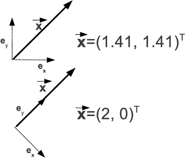
An illustration on the dependency of the components of a given vector →x on the choice of unit vectors →ei. While the vector →x does not change in the upper and lower illustration, the unit vectors span a different coordinate system, resulting in different components of the very same vector.
Let’s consider an arbitrary function f(x1,...,xn) a vector in a coordinate system spanned by an infinite number of base functions ei(x1,...,xn). It may be hard to imagine a coordinate system of infinite dimension spanned by functions. I can’t do that either. But it is also not necessary since a few things remain valid for such a coordinate system. If it is to be orthonormal, the base functions have to fulfill Equation 5.13. We can then compute the contribution of each base function ei(x1,...,xn) to the function f(x1,...,xn) by computing the inner product of the two. The question that remains is the definition of an inner product for functions. A possible definition is the integral of a product of functions:
f(x1,...,xn)·g(x1,...,xn)=∞∫−∞dx1...dxnf(x1,...,xn)g*(x1,...,xn) (5.16)
g*(x1,...,xn) is the complex conjugate of g(x1,...,xn); we will learn more about this operation in Section 5.2.2. The orthogonality requirement from Equation 5.13 can therefore be rewritten as
∞∫−∞dx1...dxnei(x1,...,xn)e*j(x1,...,xn)δij (5.17)
After decomposing the function f(x1,...,xn) to its components - let’s call them ci as the xi are the variables - the function can be written as:
f(x1,...,xn)=∞∑i−0ciei(x1,...,xn) (5.18)
We can compute the coefficients ci like in Equation 5.15:
ci=∞∫−∞dx1...dxnf(x1,...,xn)e*i(x1,...,xn) (5.19)
Usually, we hope that the components ci of higher order i do not contribute much, and that the series can be truncated after a while.
A large number of different functions fulfilling Equation 5.17 exists, and one can even design special ones. If we have such a functional system, we can always decompose an arbitrary function f(x1,...,xn) into its components in the coordinate system spanned by the base functions ei(x1,..., xn). The usefulness of such an operation lies in the choice of the base function set ei(x1,...,xn). Remember that mathematical problems can be simplified by choosing the appropriate coordinate system such as polar coordinates. Here, it is just the same. A function that shows radial symmetry can be expanded in a series of base functions that exhibit a radial symmetry themselves; since base functions are very often polynomials, a simplification of the mathematical problem to be tackled is usually the consequence.
One may object that computing the integral from Equation 5.16 will be extremely cumbersome - but we are talking about image processing here, where all functions are given as discrete values. Computing an integral in discrete mathematics is as simple as numerical differentiation. The integral is simply computed as the sum of all volume elements defining by the function. The mathematical ∫ sign becomes a Σ, and ∞ becomes the domain where the function is defined. Things that look pretty scary when using mathematical notation become rather simple when being translated to the discrete world.
So what is the purpose of the whole excursion? In short terms, it can be very helpful to describe a function in a different frame of reference. Think of the Cartesian coordinate system. If we are dealing with a function that exhibits a rotational symmetry, it may be very helpful to move from Cartesian coordinates with components xi to a polar or spherical coordinate system, where each point is given by r - its distance from the origin of the coordinate system - and φ, the angle enclosed with the abscissa of the coordinate system (or two angles if we are talking about spherical coordinates). The same holds true for functions, and in Section 5.2.2, we will examine a set of extremely useful base functions in a painstaking manner.
5.2.2 Waves - a special orthonormal system
Jean Baptiste Joseph Fourier, orphan, soldier and mathematician, studied the problems of heat transfer, which can be considered a diffusion problem. In the course of his efforts, he formulated the assumption that every periodical function can be decomposed into a series of sines and cosines. These Fourier Series are built like in Equation 5.18, using coskx, k = 0,1,... and sin kx, k = 0,1,... as base functions. The inner product is defined similarly to Equation 5.16 by f(x)·g(x)=fπ−πdxf(x)g(x). Orthogonality relations like Equation 5.17 can be proven, and we end up with the series expansion
f(x)=a02+∞∑k=1akcos kx+∞∑k=1bksin kx (5.20)
with Fourier coefficients
ak=1ππ∫−πdxf(x)cos kx,bk=1ππ∫−πdxf(x)sin kx (5.21)
A few more things are necessary to unveil the power and the beauty of the Fourier-expansion; first of all, we should remember complex numbers. Real numbers have a blemish. For each operation like addition and multiplication, there exists an inverse operation. When carrying out the multiplication operation ab = c on real numbers a and b, we can invert the operation: ca=b. The same holds true for addition. But multiplication also features a pitfall. When a computing the square of a real number - let’s say d2, we do also have an inverse operation (the square root), but the result is ambiguous. If d is negative, we won’t get d as the result of √d2 - we will get |d|. In general, it is even said sometimes (by the timid and weak such as cheap hand-held calculators) that one cannot compute the square root of a negative number. This is, of course, not true. We just have to leave the realm of real numbers, just as we had to move from natural numbers to rational numbers when dealing with fractions. Man has known this since the sixteenth century when complex numbers were introduced. A central figure in complex math is the complex unit i. It is defined as the square root of −1. A complex number c is usually given as c = a + ib. In this notation, a is referred to as the real part, and b is the imaginary part of c; a complex number is therefore represented as a doublet of two numbers, the real and the imaginary part.
Complex numbers have a number of special properties; the most important ones are listed below:
Addition is carried out by applying the operation to the real and imaginary part separately.
Multiplication is carried out by multiplying the doublets while keeping in mind that i2 = −1.
Complex conjugation, of which you already heard in Section 5.2.1. It is a very simple operation which consists of switching the sign of i, and it is denoted by an asterisk. In the case of our complex number c, the complex conjugate reads c* = a - ib.
The norm of a complex number: ||c||√a2+b2. The norm operator yields a real number.
The Real and Imaginary operator. These return the real and the imaginary part separately.
The one identity that is of the utmost importance for us is the following; it is called Euler’s formula:
eiφ=cos φ+isin φ (5.22)
Complex numbers can be represented using a Cartesian coordinate system in the plane; the real part is displayed on the x-axis, whereas the y-axis shows the imaginary part. The length r of the vector is the norm. In the representation c = a + ib for a complex number, a and b represent the Cartesian coordinates; in polar coordinates, where r and φ - the angle enclosed with the abscissa - are given to represent a complex number, c can be rewritten as c = reiφ using Equation 5.22. This representation in the complex plane is also shown in Figure 5.15.
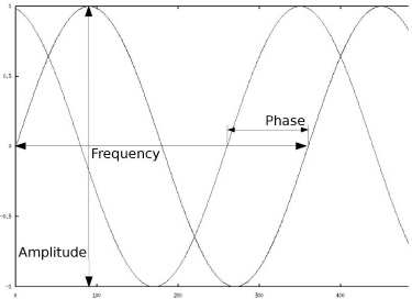
Two sines, which may be considered simple plane waves; the two variables that influence the shape of the sine are its frequency, and its amplitude. Furthermore, we have a second sine here with identical frequency and amplitude, but with a different phase. Periodical signals can be composed out of such simple waves with different frequencies, amplitudes and phases. The Fourier-transformation is a mathematical framework to retrieve these components from such a superimposed signal. Images can be considered 2D or 3D signals, and therefore it is possible to decompose them to simple planar signals as well. The sum of all frequencies and amplitudes is the spectrum of the signal.
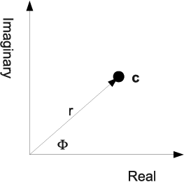
The representation of a complex number c = a + ib in the complex plane, where the real part a is represented on the abscissa and the imaginary part b lies on the ordinate. Switching to polar coordinates using r and φ and using Equation 5.22 we get another representation for a complex number: c = reiφ.
Equation 5.22 is of great importance, since it allows for a complex representation of the Fourier series using the inner product f(x)•g(x)=π∫−πdx f(x)g*(x) and the base functions eikx, k = −∞,...∞, which represent actually the plane waves.
f(x)=1√2π∞∑k=−∞ckeikx (5.23)
with Fourier coefficients
ck=1√2ππ∫−πdxf(x)e−ikx (5.24)
As you may see we have a little mess with our prefactors. In Equation 5.21 it was 12π, now it is −12π, but both in front of the sum Equation 5.23 and the Fourier coefficients Equation 5.24. The prefactors are chosen to get simpler formulas, but are unfortunately not consistent in the literature (as we know, beauty is in the eye of the beholder).
With a limiting process, which we cannot describe in detail, the sum in Equation 5.23 becomes an integral, the sequence ck becomes a function c(k) (which we will denote by ˆf(k) from now on), and the limits of the integrals in Equation 5.24 become −∞, and ∞. We can therefore define the Fourier-transform of an arbitrary function f(x) as:
ˆf(k)=1√2π∫∞−∞dxf(x)e−ikx (5.25)
f(x)=1√2π∫∞−∞dxˆf(k)eikxk...Wave number (5.26)
The similarity to Equation 5.23 and therefore to Equation 5.19 is obvious. The Fourier transformation is an inner product of the function f(x) with the base functions e−ikx. The wave number k is related to the wavelength λ of a wave by k2πλ; the wavelength by itself is related to the frequency ν as λ=cν where c is the propagation speed of the wave. A particular wave number kn is therefore the component of the function f(x) that is connected to a wave e−iknx. The Fourier-transformation is therefore a transformation to a coordinate system where the independent variable x is replaced by a complex information on frequency (in terms of the wave number) and phase. The space of the Fourier transform is therefore also referred to as k-space.
If we want to use the Fourier-transformation for image processing, we have to take two further steps. First of all, we will replace the integrals by sums. This is called the discrete Fourier transformation (DFT). Second our images are of finite size – they are not defined on a domain from −∞ to ∞. This problem can be resolved by assuming that the images are repeated, just like tiles on a floor. This is illustrated in Figure 5.16. This assumption also has visible consequences, for instance in MR-imaging. In an MR-tomograph, the original signal is measured as waves (in k-space), and is transformed to the spatial domain (the world of pixels and voxels) by means of a Fourier-transform. Figure 5.17 shows an MR image of a wrist. The hand moves out of the field-of-view of the tomograph. What occurs is a so called wraparound artifact. The fingers leaving the image on the right side reappear on the left side of the image. The principle of the discrete Fourier transformation is also shown in Figure 5.16.
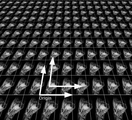
When applying a Fourier transformation to an image of finite size, it is assumed that the image is repeated so that the full spatial domain from −∞ to ∞ is covered. An image, however, has a coordinate origin in one of the image corners; in order to establish symmetry, MATLAB provides a function called fftshift. This function shifts the origin of the coordinate system to the center of the image.

A wraparound artifact in MRI. In this dynamic sequence of a wrist in motion, a part of the hand lies outside the field-of-view. Since reconstruction of volumes in MR takes place using a Fourier transformation of the original signal, the image continues like a tile so that the transformation is defined on the whole spatial domain from −∞ to ∞ - see also Figure 5.16. The right part of the hand therefore re-appears on the left side of the image. Image data courtesy of the Dept. of Diagnostic Radiology Medical University Vienna.
When applying a DFT, Equations 5.25 and 5.26 are expressed as discrete sums, rather than the clumsy integrals. Fortunately, this was already handled in a procedure called the Fast Fourier Transformation (FFT), which became one of the most famous algorithms in computer science. We can therefore always perform a Fourier transformation by simply calling a library that does a FFT, and there is quite a number of them out there. In MATLAB, a discrete FFT of a 2D function I(x,y) is carried out by the command fft2. Equation 5.26 is performed by calling ifft2. Example 5.4.6.1 gives a first simple introduction to the Fourier-transformation, where a sine is overlaid by a second sine of higher frequency. As you can see from Figure 5.29, the two frequencies of the two sines show up as four spikes, with their amplitude governing the height of the k-value in the Fourier domain. It is four spikes since a sine of negative frequency may also produce the same signal - furthermore, our initial signal, which is defined on a domain x ∈ [0,2π] has to be shifted to x ∈ [−π, π] since the Fourier transformation is defined on an interval -∞ ... ∞, not on 0 ... ∞. This is done by calling the fftshift function whose principle is illustrated in Figure 5.16.
After all these theoretical considerations, we may get to business. We know what the Fourier transformation is, and we know how to compute it. So what is the merit of the Fourier transform in image processing? Since an image is a function defined on the 2D or 3D domain, it can be decomposed to plane or spherical waves; noise, for instance, is a signal with a high frequency. If we want to get rid of noise, we may reduce the weight of the higher frequencies (the components with a large value of the wave number k). If we want to sharpen the image, we can emphasize the higher frequencies. These operations are therefore obviously equivalent to Kblur and Ksharp, which were already called high-pass and low-pass filters. The advantage of blurring and sharpening in the Fourier domain, however, is the possibility to tune the operations very specifically. We can select various types of noise and remove it selectively, as we will do in Example 5.4.6.1. Furthermore, the Fourier transformation has some remarkable properties, which are extremely handy when talking about filtering operations beyond simple manipulation of the image spectrum.
5.2.3 Some important properties of the Fourier transform
The Fourier transformation has some properties of particular interest for signal and image processing; among those are:
Linearity: w*f+g↦w*ˆf+ˆg.
Scaling: Doubling the size of an image in the spatial domain cuts the amplitudes and frequencies in k-space in half.
Translation: f(x+α)↦ˆf(k)eikα. A shift in the spatial domain does not change the Fourier transform ˆf(k) besides a complex phase. This property is also responsible for so-called ghosting artifacts in MR, where motion of the patient during acquisition causes the repetition of image signals (see also Figure 5.18).
Convolution: f(x)*g(x)↦√2π*ˆf(k)*ˆg(k). As you may remember from the introduction to this chapter, it was said that the convolution operation by mangling kernels into the image will be replaced by a strict and simple formalism. Here it is. In k-space, the convolution of two functions becomes a simple multiplication. Therefore, it is no longer necessary to derive large kernels from a function such as the Gaussian as in Equation 5.3.
Differentiation: dndxnf(x)↦(ik)nˆf(k). Computing the derivative of a function f(x) is apparently also pretty simple. Again it becomes a simple multiplication.
The Gaussian: The Gaussian G(x) retains its general shape in k-space. Under some circumstances, is even an eigenfunction of the Fourier transform;4 in general, however, ˆG(k) is a Gaussian as well.
Parseval’s Theorem: The total energy in the image, which can be considered the sum of squares of all gray values ρ, is maintained in k-space. Another formulation is f·g↦ˆf·ˆg.

The translation property of the Fourier transform at work. As said before, the MR signal is acquired in k-space and transformed to the spatial domain for volume reconstruction. When patient motion during image acquisition occurs, the result is the repetition of image structures in the reconstructed volume (see arrow). This T2-weighted image of the pelvis was windowed in such a manner that the ghosting artifact - the repetition of the abdominal wall in the upper part of the image - becomes prominent. Ghosting artifacts in this area of the body are common due to breathing motion. Image data courtesy of the Dept. of Radiology Medical University Vienna.
Another important theorem that is connected to the DFT is the Nyquist-Shannon Sampling Theorem. In the DFT, the sampling frequency has to be double the highest frequency of the signal to be reconstructed - if, for instance in an audio signal, the highest frequency is 20 kHz (which is the maximum frequency man can hear), the sampling frequency has to be 40 kHz for a lossless reconstruction of the signal.
From this little excursion, it should be clear why the Fourier transformation is considered such a powerful tool in signal processing. In the next sections, we will learn how to apply the Fourier transform to medical images. A first example on the conditioning of signals named Rect 5.m can be found in the LessonData folder. The power spectrum of a more complex function - the mouse topogram from Figs. 5.10 and 5.11 - is given in Figure 5.19.
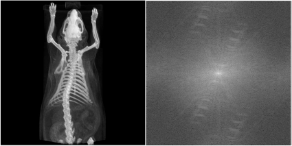
The topogram of a mouse taken from small animal CT, and the absolute value of the Fourier-spectrum after a logarithmic intensity transform. Some of the details in the left image from the spatial domain leave a recognizable trace in the spectrum on the right-hand side. For instance, the low frequencies in the y-direction are more dominant than in the x-direction since the mouse occupies more space in the y-direction. Furthermore, the ribcage gives a significant signal of high intensity at a higher frequency, and the bow-shaped structures in the medium frequency range indicate this. Image data courtesy of C. Kuntner, AIT Seibersdorf, Austria.
5.2.4 Image processing in the frequency domain
From Example 5.4.6.1, we will see that we can get rid of image noise with a known frequency. In medical imaging, such periodical artifacts may also occur, for instance in MR - imaging, or in CR plates, which may be stricken by discretization artifacts. An example of a band-stop filter, which removes some of the middle frequencies in the image, is given in Example 5.4.7. Of course, we can also introduce blurring and sharpening by removing the high or low frequencies in the image (Figure 5.36). The maximum wave number k, which represents the highest frequency in the image, is defined by the resolution of the image since the smallest signal given in the image is a single point.
Another important property of the Fourier-transformation is the convolution-operation; remember Section 5.1.1, where small 2D-functions like Kblur were convolved with the image. In k-space, convolution becomes a multiplication. We can convolve kernels of all kinds (some of them have names such as Hann, Hamming, Butterworth and so on) by simply transforming both the kernel and the image to k-space, and multiply the two. After re-transformation to the spatial domain, we get the effect of the convolution operation. This may look like artificially added complexity, but the operation is actually way more simple than convolution in the spatial domain when it comes to more complicated kernels. One may remember K5×5 Gauss from Equation 5.3, where a simple 5 × 5 kernel already requires 25 operations per pixel for convolution. Furthermore, we can invert the convolution operation; if we know the exact shape of our PSF, we can apply the inverse process of the convolution operation in k-space, which is actually a multiplication with the inverse of the PSF. This process is called deconvolution or resolution recovery.
Next, we know that translation of the image just introduces a complex phase in k-space. When taking a look at the norm of a shifted function f(x + α) in k-space, we will have to compute ˆf(k)eikα(ˆf(k)eikα)* - the product of the transformed function ˆfeikα and its complex conjugate. For complex conjugation, the identity (c1c2)*=c*1c*2 is true. The norm of a shifted function in k-space therefore reads ˆfˆf* - the complex phase introduced by the shift in the spatial domain disappears. An image and a shifted image can therefore be identified as one and the same besides the shift if one compares the norm of the Fourier-transforms of the image. This is especially handy in image registration, which will be introduced in Chapter 9.
5.2.5 Modelling properties of imaging systems - the PSF and the MTF
Let us go back to the introduction, where an optical system was introduced as a filter. The quality of the PSF, as we may recall, gives an idea of the overall performance of the system since it can be convolved with an arbitrary signal; if we leave the domain of medical images, we can encounter an excellent example in Figure 5.20. This is the globular cluster M13 in the constellation of Hercules, a collection of old stars at the edge of our galaxy. It contains hundreds of thousands of stars. From a signal processing perspective, the image of each star is the result of the convolution with the PSF of the telescope. The interesting question is -how does the PSF, or the optical quality of the telescope, affect the resolution of the image? How close can two stars, which are pretty perfect examples for distant point light sources, be in order to be resolved as separate? The ability to distinguish two point sources depending on their distance is given by the so-called modulation transfer function (MTF). The MTF gives a score whether the two images overlap as a function of the spatial frequency that separates the two PSF-like images in term of cycles over range. It is obvious that a bad optical system with a large PSF such as the spherical mirror introduced in Figure 5.2 will not resolve nearby objects since the PSFs would overlap. Figure 5.21 shows the MTF of the spherical mirror that gives the PSF from Figure 5.2. The question therefore is – what is the exact relationship of the PSF and the MTF?

M13, the great globular cluster in the Hercules constellation. The ability to resolve two stars as separated depends on the PSF of the optical system used. In a poor optical system like the spherical mirror presented in the introduction, the image would not look like that since the amount of overlap between two images of the nearby stars would fuse them. The ability to distinguish two close objects is measured by the modulation transfer function, the MTF.
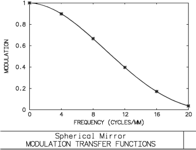
The modulation transfer function of the spherical mirror from Figure 5.2. The graph was, again, produced using the OSLO optical design software. The MTF gives a figure of the capability of a signal-transducing system to resolve two point-shaped objects. The higher the spatial frequency (given in cycles/mm in the image plane in this example), the lower the resolution of the system. The MTF is coupled to the PSF by means of the Fourier-transformation; a wide PSF gives a narrow MTF and vice versa.
The answer is not very surprising. The MTF is the absolute value of the Fourier-transform of the PSF. This is illustrated in Example 5.4.8. The mouse image MouseCT.jpg, already misused many times for all types of operations, is convolved with Gaussian PSFs of varying width. A narrow Gaussian will not distort the image a lot – fine detail will remain distinguishable; therefore the MTF is wide. While the Fourier-transform of a narrow Gaussian is still a Gaussian, it becomes a very wide distribution. Figure 5.39 illustrates this. If we apply a wide Gaussian PSF, the MTF will become narrow since fine details vanish. In Example 5.4.8, this will be demonstrated. It is noteworthy that a measurement of the PSF is a common task in the maintenance of medical imaging systems such as CTs, where dedicated phantoms for this purpose exist. Example 5.4.9 illustrates such an effort.
5.3 Other Transforms
An infinite number of orthonormal base function systems ei(x1, ..., xn), which are usually polynomials, can be constructed. Whether a transform to these systems makes sense depends on the basic properties. If it is of advantage to exploit the rotational symmetry of an image, one may compute the representation of the image in a base system that shows such a symmetry. Jacobi polynomials are an example for such a base system. Another example of a particularly useful transformation is real-valued subtype of the discrete Fourier transform, the discrete cosine transform (DCT). The DCT is, for instance, used in JPG-compression (see also Chapter 3). For now, we will stop dealing with these types of transformations, and we will introduce two important transforms that are not based on orthonormal base functions.
5.3.1 The Hough transform
The Hough transform is a transformation that can be used for any geometrical shape in a binary image that can be represented in a parametric form. A classical example for a parametric representation is, for instance, the circle. A circle is defined by the fact that all of its points have the same distance r from the center of the circle (Mx,My). A parametric representation of a circle in a Cartesian coordinate system is given as:
√(x−Mx)2+(y−My)2=r.
Center coordinates Mx, My and radius r are the parameters of the circle. We will make use of this representation in a number of examples, for instance Example 6.8.5 and 7.6.4. As a parametric representation of a straight line we choose the Hesse normal form. It is simply given by the normal vector of the line which intersects with the origin of a Cartesian coordinate system. An illustration is given in Figure 5.22. The parameters are the polar coordinates of this normal vector →n. The Hough transform inspects every non-zero pixel in a binary image and computes the polar coordinates of his pixel, assuming that the pixel is part of a line. If the pixel is indeed part of a line, the transform to polar coordinates will produce many similar parameter pairs.
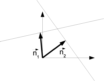
The Hesse normal form representation of lines in a Cartesian coordinate system. Each line is represented by a normal vector →n that intersects the origin of the coordinate system. The polar coordinates of the intersection point of →n and the line are the parameters of the line.
The trick in the case of the Hough transform is to plot the parameters of the shape in a new coordinate system which is spanned by the two parameters of the normal form, the length r of the normal vector →n and the angle φ enclosed by →n and the x-axis. Pixels belonging to a line will occupy the same location in Hough-space. Since the Hough transform acts only on binary images, the varying brightness of points in Hough-space is a measure of the number of pixels with the same normal vector. In Example 5.4.10, we will apply the Hough-transform to the image shown in Figure 5.44.
The result of the transformation to the parameter space can be found in Figure 5.46. The pixels that lie on a line appear as bright spots in the image. By setting all pixels below a given threshold to zero, only the bright spots in the parameter image remain. Next, one can define a so-called accumulator cell; this is a square in parameter space which assigns a single parameter pair to the area in the parameter space covered by the accumulator, thus narrowing down the number of possible parameters. While the detection of lines is a classical example of the Hough-transform, the principle is applicable to every shape that can be modeled in a parameter representation. In Chapter 10, we will encounter a very similar transformation. In medicine, the Hough transform can also be very helpful in identifying structures in segmented images, for instance when identifying spherical markers in x-ray images. A simplified application of the Hough-transform in segmentation can be found in Example 6.8.8.1.
5.3.2 The distance transform
Another transformation that we will re-encounter in Chapter 9 is the distance transform. It also operates on binary images; here, the nearest black pixel for each non-black pixel is sought. The value of the non-black pixel is replaced by the actual distance of this pixel to the next black pixel. A very simple example can be found in Figure 5.23, which is the output of Example 5.4.11.

The result of the distance transform as carried out in Example 5.4.11. The innermost pixels of the rectangle are those with the greatest separation to the border of the rectangle; therefore they appear as bright, whereas the pixels closer to the border become darker.
5.4 Practical Lessons
5.4.1 Kernel – based low pass and high pass filtering
In the SimpleLowPass_5.m script, a single CT slice in DICOM format named SKULLBASE.DCM is opened, and a simple smoothing filter Kblur is applied. The results of this script can be seen in Figs. 5.3, 5.4, and 5.24. The DICOM-file is read in the same manner as in Example 3.7.2. In order to cope with the indexing conventions of MATLAB and Octave, the image is transposed. Finally, memory for a second image lpimg is allocated.
1:> fp=fopen(’SKULLBASE.DCM’, ’r’);
2:> fseek(fp,1622,’bof’);
3:> img=zeros(512,512);
4:> img(:)=fread(fp,(512*512),’short’);
5:> img=transpose(img);
6:> fclose(fp);
7:> lpimg=zeros(512,512);

The original image SKULLBASE.DCM, and the result of the filtering operation in SimpleLowPass_5.m. Noise such as the reconstruction artifacts visible in the air surrounding the head is suppressed. Since the details are subtle and are hard to recognize in print, you may also inspect the JPG-images used for this illustration. These can be found in the LessonData folder for this chapter, and are named SKULLBASE_Filtered.jpg and SKULLBASE_Original.jpg. Image data courtesy of the Dept. of Radiology, Medical University Vienna.
Next, we will visit each pixel and convolve the image with the smoothing kernel Kblur. In order to avoid indexing conflicts, we leave the edges of the image untouched. Finally, the image intensities are shifted and scaled for an optimum representation, just like in Example 4.5.1.
8:> for i=2:511
9:> for j=2:511
10:> lpimg(i,j) = 0.1*(img((i-1),j) + 2*img(i,j) +
img((i+1),j) + img(i,(j-1)) + img(i,(j+1)) +
img((i-1),(j-1)) + img((i-1),(j+1)) +
img((i+1),(j-1)) + img((i+1),(j+1)));
11:> end
12:> end
13:> minint=min(min(lpimg));
14:> lpimg=lpimg-minint;
15:> maxint=max(max(lpimg));
16:> lpimg=lpimg/maxint*64;
17:> colormap(gray);
18:> image(lpimg)
Additional Tasks
Modify SimpleLowPass_5.m in such a manner that it utilizes the 5×5 Gaussian kernel from Equation 5.3, and compare the results.
Modify SimpleLowPass_5.m to sharpen the image using the Ksharp kernel from Equation 5.2. A detail from the result can be found in Figure 5.4. A high pass filter can be somewhat difficult for images with negative pixel values like CT image data due to the negative values in the Ksharp kernel.
As one may see from this script, a generalization to the 3D domain is pretty straightforward and simple. The kernel Kblur can easily be generalized to average the gray values in neighboring voxels. What would a 3D-equivalent of Kblur look like?
It was already stated in the introduction, a prerequisite for applying kernels like Kblur is an isotropic image. Can you think of a kernel that properly operates on an image where the pixels are stretched by a given ratio?
5.4.2 Basic filtering operations in ImageJ
One of the strengths of ImageJ is the fact that it can be easily expanded by plugins. The built-in functionality is therefore somewhat limited; however, the basic filtering operations that can be found in ImageJ are smoothing, sharpening and edge detection using the length of the image gradient as determined by a Sobel filter (see also Figure 5.25). Basically, the three filtering operations that can be found under the Menu topics “Process → Smooth”, “Process → Sharpen” and “Process → Find Edges” correspond to the application of the kernels Kblur – Equation 5.1, Ksharp – Equation 5.2 and the length of the gradient as determined by KSobelx and KSobely – Equation 5.9 to the image LowDoseCT.tif from the LessonData folder. The image is a slice from a whole-body CT scan taken in the course of a PET-CT exam; since the dose applied in a PET-CT exam is considerable (up to 25 mSv), the CT is a so-called low-dose CT with considerable image noise. This is especially evident after using the sharpening and the edge-detection filter (see Figure 5.26).

Screenshot of ImageJ; in the “Process” menu, basic operations such as smoothing, sharpening and edge detection using Sobel-kernels can be found.

Effect of blurring (or “smoothing”), sharpening, and edge detection on the image file LowDoseCT.tif from the LessonData folder. The image is part of a PET-CT scan; since the whole patient was scanned, the radiologist in charge chose a low dose CT protocol, which results in considerable noise in the image. The design of the filter kernels used here is similar to the kernels presented in Section 5.1.1. Image data courtesy of the Dept. of Radiology, Medical University Vienna.
5.4.3 Numerical differentiation
In this example, we are dealing with two scripts. The first one illustrates numerical forward differentiation on a simple one dimensional rectangle function. It is named NumericalDifferentiation_5.m.
1:> rect=zeros(100,1);
2:> for i=45:55
3:> rect(i,1)=1;
4:> end
5:> plot(rect);
6:> foo=input(’Press RETURN to proceed to the first derivative’);
rect is the vector containing the dependent variable of the rectangle function, which is zero for x ∈ 1... 44 and x ∈ 56 ... 100, and one otherwise. This function is plotted, and after an old-fashioned command line prompt, the script proceeds:
7:> drect=zeros(100,1);
8:> for i=1:99
9:> drect(i,1)=rect(i+1)-rect(i);
10:> end
11:> plot(drect)
12:> foo=input(’Press RETURN to proceed to the second derivative’);
The first derivative, df(x)dx, is computed. As you can see, it is a simple forward difference. The df(x) term becomes affinite difference, f(xi+1) - f(xi), and the denominator is 1 since we are dealing with discrete values for x that increment by one. The second derivative, d2f(x)dx2, is computed in the same manner. The forward differences of the drect vector yield a vector ddrect, which contains the second derivative.
13:> ddrect=zeros(100,1);
14:> for i=1:99
15:> ddrect(i,1)=drect(i+1)-drect(i);
16:> end
17:> plot(ddrect)
The output of this operation can be found in Figure 5.6. Interpreting the derivative is simple. Whenever the slope of the original function f(x) is steep, the numerical value of the derivative is high. If we encounter a descent in the function, the derivative has a high negative value.
In terms of image processing, edges in the image are steep ascents or descents; forming the derivatives will give sharp spikes at these edges, visible as very dark or very bright lines in the resulting image. Numerical differentiation is therefore the easiest way to detect edges in images. The second script, named ForwardDifference_5.m, implements the simple differentiation kernel Kx-forward from Equation 5.5. Otherwise, it is largely identical to SimpleLowPass_5.m.
1:> fp=fopen(’SKULLBASE.DCM’, ’r’);
2:> fseek(fp,1622,’bof’) ;
3:> img=zeros(512,512);
4:> img(:)=fread(fp,(512*512),’short’) ;
5:> img=transpose(img);
6:> fclose(fp);
7:> diffimg=zeros(512,512);
Since we are computing a forward difference, the indexing may start from i=1, as opposed to the SimpleLowPass_5.m script. The result of the convolution operation, diffimg is, as usual, scaled to 6 bit depth and displayed. The result can be found in Figure 5.7.
8:> for i=1:511 9:> for j =1 : 511
10:> diffimg(i,j) = -img(i,j) + img(i+1,j);
11:> end
12:> end
13:> minint=min(min(diffimg)) ;
14:> diffimg=diffimg-minint;
15:> maxint=max(max(diffimg)) ;
16:> diffimg=diffimg/maxint*64;
17:> colormap(gray);
18:> image(diffimg)
Additional Tasks
Implement Ky-forward, and inspect the result.
What would Kx-backward look like? Implement it and compare the result to the out-come of ForwardDifference_5.m.
Since we are interested in edges only, we can also implement a version of Kx-forward which takes absolute values of the derivative only. The result should look like the right hand image in Figure 5.7.
Implement the operation for total differentiation using Equation 5.8. The result is found in Figure 5.8. The Sobel_5.m script in the LessonData folder implements a Sobel filter. Compare the outcome, which can also be found in Figure 5.27 by subtracting the resulting images from each other prior to scaling the images to 6 bit depth.
The result of applying a Sobel-filter to SKULLBASE.DCM. The reader is encouraged to compare this image to the corresponding image in Figure 5.8. Image data courtesy of the Dept. of Radiology Medical University Vienna.
5.4.3.1 A note on good MATLAB® programming habits
By using MATLABs vector notation, lines 2 - 4 in NumericalDifferentiation_5.m can be replaced by:
...:> rect(45:55,1)= 1;
5.4.4 Unsharp masking
The UnsharpMask_5.m script is mainly derived from SimpleLowPass_5.m script; it implements the kernel for unsharp masking as given in Equation 5.11. The beginning of the script looks familiar. Besides the low pass filtered image lpimg, we reserve the memory for a second image uming, and a constant factor weight is defined:
1:> fp=fopen(’SKULLBASE.DCM’, ’r’);
2:> fseek(fp,1622,’bof’);
3:> img=zeros(512,512);
4:> img(:)=fread(fp,(512*512),’short’);
5:> img=transpose(img);
6:> fclose(fp);
7:> lpimg=zeros(512,512);
8:> umimg=zeros(512,512);
9:> weight=1;
Now, the low pass filtered image using Kblur is computed, and the unsharp masking kernel is applied according to Equation 5.11.
10:> for i=2:511
11:> for j=2:511
12:> lpimg(i,j) = 0.1*(img((i-1),j) + 2*img(i,j) +
img((i+1),j) + img(i,(j-1)) + img(i,(j+1)) +
img((i-1),(j-1)) + img((i-1),(j+1)) +
img((i+1),(j-1)) + img((i+1),(j+1)));
13:> umimg(i,j) = img(i,j) - weight*lpimg(i,j);
14:> end
15:> end
Finally, the whole image is scaled to 6 bit depth as we have done so many times before.
16:> minint=min(min(umimg));
17:> umimg=umimg-minint;
18:> maxint=max(max(umimg));
19:> umimg=umimg/maxint*64;
20:> colormap(gray);
21:> image(umimg)
Additional Tasks
Experiment with different constants weight and inspect the image.
We have learned that the convolution operation is linear – therefore it should be possible to compute KUnsharp Mask as a single kernel, and apply that kernel to the image instead of computing lpimg. Derive the kernel and implement it. Does the result look the same as from UnsharpMask_5.m?
5.4.5 The median filter
In the MedianFiveTimesFive_5.m script, a median filter is implemented. The beginning is similar to the other scripts in this chapter. Again, SKULLBASE.DCM is read, and a matrix for the resulting image is reserved:
1:> fp=fopen(’SKULLBASE.DCM’, ’r’);
2:> fseek(fp,1622,’bof’);
3:> img=zeros(512,512);
4:> img(:)=fread(fp,(512*512),’short’);
5:> img=transpose(img);
6:> fclose(fp);
7:> mfimg=zeros(512,512);
Next, a vector rhovect is reserved, which holds all the gray values ρ in the 25 pixels which form the kernel of the 5 × 5 median filter. These values are stored, and the vector is sorted by calling the sort function of MATLAB (whose function is self-explaining). After sorting the vector rhovect, the median is computed as the central element of this rank list. Since we have 25 entries in rhovect, the central element is located at position 13. The weak may be tempted to use the median function of MATLAB, which does essentially the same:
8:> rhovect = zeros(25,1);
9:> for i=3:510
10:> for j=3:510
11:> idx = 1;
12:> for k = -2:2
13:> for l = -2:2
14:> rhovect(idx)=img((i+k),(j+l));
15:> idx = idx + 1;
16:> end
17:> end
18:> rhovect=sort(rhovect);
19:> mfimg(i,j) = rhovect(13,1);
20:> end
21:> end
Finally, we will again scale the image to 6 bit depth, and display the result using the image function; Figure 5.28 shows the result.
22:> minint=min(min(mfimg));
23:> mfimg=mfimg-minint;
24:> maxint=max(max(mfimg));
25:> mfimg=mfimg/maxint*64;
26:> colormap(gray);
27:> image(mfimg)
The result of a 5×5 median filter as performed in Example 5.4.5. The median filter suppresses noise and does also blur the image like a linear low-pass filter. However, it is robust to outliers by definition, and it tends to retain overall structural information to a larger extent compared to linear smoothing filters, as already shown in Figure 5.10. Image data courtesy of the Dept. of Radiology, Medical University Vienna.
Additional Tasks
Enhance the filter to an 11 × 11 median filter.
Can you imagine what a maximum and a minimum filter is? Implement them based on MedianFiveTimesFive_5.m.
5.4.6 Some properties of the Fourier-transform
5.4.6.1 Spectra of simple functions in k-space
In order to become familiar with the Fourier transform, we will take a closer look at the effects of the FFT on a well known function, the sine. The script Sine_5.m can be found in the LessonData folder. First, a sine function for angles x from 0 to 360 degrees is plotted; we do, of course, use radians. A second sine wxx with a frequency hundred times higher, but with only a tenth of the amplitude of wx is generated as well and added to the sinusoidal signal wx, resulting in a signal y. Again, the good old command-line prompt halts the script until you are satisfied inspecting the resulting function in the spatial domain.
1:> x=1:360;
2:> wx=sin(x*pi/180);
3:> rattlefactor = 0.1;
4:> wxx=rattlefactor*sin(x*100*pi/180);
5:> y=wx+wxx;
6:> plot(y)
7:> foo=input(’Press RETURN to see the spectrum ...’);
The signal y is transformed to k-space using the built-in fft command, and shifted to a symmetric origin using fftshift. The absolute value of the complex spectrum is displayed, and the script is halted again.
8:> fy=fft(y);
9:> fys=fftshift(fy);
10:> plot(abs(fys))
11:> foo=input(’Press RETURN to see the filtered spectrum...’);
By removing the part of the spectrum that contains the additional signal wxx, we get the signal of the original sine signal wx. Again, the absolute value of the complex spectrum is displayed.
12:> for i=70:90
13:> fys(i)=0;
14:> fys(200+i)=0;
15:> end
16:> plot(abs(fys))
17:> foo=input(’Press RETURN to see the filtered sine in the spatial domain...’);
Finally, we transform the cleaned spectrum back to the spatial domain, and look at the result, which is a sine function without added noise. The function to perform an inverse Fourier transformation in MATLAB is called ifft. Since we also have to re-establish the origin of the image coordinate system, the inverse operation for fftshift called ifftshift has to be carried out. We have not yet scaled the k-space properly, therefore the values on the k-axis of the plots for the spectra are not correct. Figure 5.29 shows the four plots generated by the script.
18:> rsine=ifft(ifftshift(fys));
19:> plot(real(rsine))

The four plots generated by the Sine_5.m script. The first plot shows the initial signal y – a sine overlaid by a smaller sine with higher frequency. The second and third plot show the absolute value of the spectrum. The frequency of the wx signal, which has a higher amplitude, is found in the middle of the plot. The higher frequency of the noise wxx is further to the left and the right of the origin of the coordinate system – it is lower since the amplitude of wxx is smaller. After removal of the contributions of wxx to the spectrum, the transformation back to the spatial domain shows the signal wx without the ripple added by wxx.
5.4.6.2 More complex functions
Spectra in 1D – decomposing a chord In this example, we will apply the Fourier-transform to a sound. That is a very obvious application since sounds are, technically speaking, periodic fluctuations of air density. A sound is therefore composed out of an overlay of several waves. In your LessonData folder, you find in the sub-folder 5_Filtering three sounds named c_piano.wav, c_aguitar.wav and c_eguitar.wav. These were also stored in MPG format, and you can listen to them on your computer. All three files are recordings of the same chord – a simple C major chord. A simple major chord consists of a triad of three single notes. The first one is the root note, followed by the major third and the fifth. In the case of C major, we are talking about the notes C, e and g. These notes are generated in a different fashion on different instruments; therefore, a chord sounds different when being played on a piano or a guitar.
For the sake of simplicity, we have also converted the .wav sound files to a raw format. The sounds are read by MATLAB using the ChordSpectrum_5.mscript in the usual manner, just like we did with the DICOM files in earlier examples – the sound consists of a series of numbers with 16 bit, and these values are read into a vector called chord after opening the raw data file:
1:> clear;
2:> fp = fopen(’c_piano.raw’,’r’);
3:> chord=zeros(240630,1);
4:> chord(:)=fread(fp,240630,’short’);
5:> fclose(fp);
6:> plot(chord)
7:> ylim([-22000 22000]);
8:> foo=input(’Now proceed to the spectrum of the ... chord played on piano...’);
The command ylim (and the command xlim, which we will encounter in the next few lines of code) makes sure that the scaling of the x- and y-axis does not change when displaying the different chords. The signal now undergoes a Fourier-transform, just as we did before with other signals:
9:> kpchord=abs(fftshift(fft(chord)));
10:> plot(kpchord);
11:> xlim([100000 140000])
The remainder of the script is very straightforward; we repeat the same procedure for the C major chord played on acoustic guitar and on a mighty electric guitar. The result can be found in Fig. 5.30.

The results of ChordSpectrum_5.m, where a C major chord played on piano, acoustic and electric guitar is displayed as a power spectrum. The differences – showing the different contributions in amplitude and harmonics – are clearly visible. The audible result is the different sound of the chord, which is also stored as an audio file in the LessonData folder.
12:> foo=input(’Now look at the chord... played on acoustic guitar...’);
13:> fp = fopen(’c_aguitar.raw’,’r’);
14:> chord=zeros(239616,1);
15:> chord(:)=fread(fp,239616,’short’);
16:> fclose(fp);
17:> plot(chord)
18:> ylim([-22000 22000]);
19:> foo=input(’Now proceed to the spectrum of the... chord played on acoustic guitar...’);
20:> kagchord=abs(fftshift(fft(chord)));
21:> plot(kagchord);
22:> xlim([100000 140000])
23:> foo=input(’Now look at the chord played ... on electric guitar...’);
24:> fp = fopen(’c_eguitar.raw’,’r’);
25:> chord=zeros(239616,1);
26:> chord(:)=fread(fp,239616,’short’);
27:> fclose(fp);
28:> plot(chord)
29:> ylim([-22000 22000]);
30:> foo=input(’Now proceed to the spectrum of the ... chord played on acoustic guitar...’);
31:> kegchord=abs(fftshift(fft(chord)));
32:> plot(kegchord);
33:> xlim([100000 140000])
From the spectra we see the subtle difference – we have decomposed the chords into their components, and we see the different contributions from the higher harmonics, which result in a different sound, despite the fact that the three chords are identical.
A Rectangle function In the Rect_5.m script, the rect-function also known from Figure 5.6 is transformed to k-space. The rect-function does not have a single frequency like the sine from Sine_5.m. Rather than that, it is composed out of many plane waves with different frequencies and amplitudes:
1:> rect=zeros(100,1);
2:> ffrect=zeros(100,1);
3:> for j=45:55
4:> rect(j,1)=1;
5:> end
6:> frect=fft(rect);
7:> frect=fftshift(frect);
In the next few lines, we remove the higher frequencies in steps of ten up to all hundred frequencies and transform the remainder back to the spatial domain. The result is the approximation of the rect-function up to a given order, just as indicated in Equation 5.18. Subsequently, the single steps are displayed using the plot function. Since the Fourier transform is complex valued, the inverse Fourier-transform yields complex numbers; however, the imaginary part of these complex numbers is zero, therefore we can use the real operator to retrieve the real part of these values in the spatial domain. The ylim command takes care of the proper scaling of the y-axis:
8:> for j = 1:4
9:> klimlow=50-j*10
10:> klimhigh=50+j*10
11:> for k=1:100
12:> if (k < klimlow) | (k > klimhigh)
13:> ffrect(k,1) = 0;
14:> else
15:> ffrect(k,1)=frect(k,1);
16:> end
17:> end
18:> rrect=ifft(ifftshift(ffrect));
19:> plot(real(rrect))
20:> ylim([-0.2 1.5])
21:> foo=input(’Press RETURN to proceed to the next rectangle pulse’);
22:> end
Additional Tasks
Implement a simple high-pass filter based on the Rect_5.m script.
Filtering a simple 2D image Let us now proceed to twodimensional signals. Figure 5.32 shows a simple black and white photography of a brickwall. To some extent, this image is similar to the 1D-rectangle function. Let us apply a 2D-Fourier transform to this image. The script is called WallFourier_Y_LP_5.m, and as usual, it can be found in the LessonData folder. First, we clear all variables from the workspace, we allocate a matrix for the 512×512 image brickwall.jpg, and we carry out a 2D Fourier transform, followed by a fftshift command that establishes a symmetry around the center of the image:
1:> clear;
2:> img=zeros(512,512);
3:> img = imread(’brickwall.jpg’);
4:> fimg = fft2(img);
5:> fimg= fftshift(fimg);

The output from script Rect_5.m. We see how the original rect-function is low-pass filtered from the Fourier spectrum. The lower the maximum order i (which is called klimlow and klimhigh in the script), the more massive the low-pass filtering.

Another not-so-medical example (it is at least a hospital wall) of a 2D image with very few frequencies. We see bricks and mortar joints here, pretty well aligned in horizontal and vertical direction. In this example, we can filter frequencies in the direction of the coordinate axes using the WallFourier_Y_LP_5.m script from the LessonData-folder.
Next, we set all the frequencies to the left and the right of a line that is parallel to the y-axis and passes through the center of the image to zero. What remains are the major frequencies in the y-direction. As a matter of fact, all elements of the image that have a major component in the x-direction are removed, leaving only the horizontal mortar joints in the image.
6:> for i=1:512
7:> for j=1:254
8:> fimg(i,j)=complex(0,0);
9:> end
10:> end
11:> for i=1:512
12:> for j=258:512
13:> fimg(i,j)=complex(0,0);
14:> end
15:> end
The only thing that is left for us is to transform the image back to the spatial domain, to scale the image intensities to 6 bit, and to display the image. The result can be found in Figure 5.33:
16:> lpimg=zeros(512,512);
17:> lpimg = real(ifft2(ifftshift(fimg)));
18:> minint=min(min(lpimg));
19:> lpimg=lpimg-minint;
20:> maxint=max(max(lpimg));
21:> lpimg=lpimg/maxint*64;
22:> colormap(gray);
23:> image(lpimg)
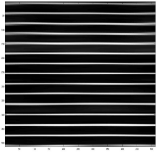
The output of WallFourier_Y_LP_5.m. All the vertical details visible in Figure 5.32 were removed by setting the frequencies that contribute in the x-direction of the image to zero.
The spectrum of a 2D image A more complex function is the mouse, already known from Figs. 5.10 and 5.11. The script MouseSpectrum_5.m performs a two-dimensional Fourier transform of the MouseCT.jpg image. The image is read, transformed using the fft2 command, and the low frequencies are shifted to the center of the matrix containing the k-values.
1:> img=zeros(733,733) ;
2:> img = imread(’MouseCT. jpg’) ;
3:> fimg = fft2(img);
4:> fimg = fftshift(fimg);
5:> psimg=zeros(733,733);
Next, we compute the norm of the power spectrum using the abs function; in order to visualize the low contrast detail in the resulting image, we apply a logarithmic transform to the resulting image, just as in Example 4.5.3, and display the result using the image command. The result can be found in Figure 5.19:
6:> for j=1:733
7:> for k=1:733
8:> psimg(j,k) = abs(fimg(j,k)) ;
9:> end
10:> end
11:> psimg = log(psimg);
12:> minint=min(min(psimg)) ;
13:> psimg=psimg-minint;
14:> maxint=max(max(psimg)) ;
15:> psimg=psimg/maxint*64;
16:> colormap(gray);
17:> image(psimg)
5.4.6.3 Convolution of simple functions
Another example can be found in the Simpleconvolution_5.m script, where a rect-function and a sawtooth are convolved. We have already performed the convolution operation on images; mathematically speaking, a convolution of two functions f(x) and g(x) is an integral: f*g(x)=∫∞−∞dyf(y)g(x−y). According to the convolution theorem, we can as well transform the two functions to k-space and simply multiply them. The re-transformation yields the convolved function. First, we draw the two functions - the rect and the sawtooth - and plot them separately:
1:> rect=zeros(100,1);
2:> for i=35:65
3:> rect(i,1)=15;
4:> end
5:> saw=zeros(100,1);
6:> for i=1:15
7:> saw(i,1)=i-1;
8:> end
9:> for i=16:29
10:> saw(i,1)=29-i;
11:> end
12:> plot(rect)
13:> ylim([-1 20]);
14:> foo=input(’Press RETURN to proceed to the sawtooth to be convolved... ’);
15:> plot(saw)
16:> ylim([-1 20]);
17:> foo=input(’Press RETURN to proceed...’);
The input function causes a program halt until the RETURN key is pressed; the ylim function, which was already used earlier, takes care of a proper scaling of the ordinate.
Next, we transform rect and saw to k-space. The convolution takes place by a component-wise multiplication of the resulting complex vectors fr and fs using the .* operator. After this operation, the resulting function fconv is transformed back to spatial domain, and the resulting function rconv is displayed.
18:> fr=fft(rect);
19:> frs=fftshift(fr);
20:> fs=fft(saw);
21:> fss=fftshift(fs);
22:> fconv=frs.*fss;
23:> fconvs=ifftshift(fconv);
24:> rconv=ifft(fconvs);
25:> plot(real(rconv))
5.4.6.4 Differentiation in k-space
Finally, we will give a simple example of differentiation in k-space. The FourierDiffRect_5.m script differentiates the rect function; the result of such an operation we have already seen in Figure 5.6. For the first time, we will try to do a proper mapping of the possible values of k. We remember that the maximum frequency (or the maximum cycles over range) are given by the number of pixels in an image, or the number of pivoting points when defining a function as a vector of numbers. First, a rect function rect is defined, just like in Example 5.4.3. The function is transformed to k-space and shifted in such a manner that the origin lies in the middle of the transformed function.
1:> rect=zeros(100,1);
2:> for j=45:55
3:> rect(j,1)=1;
4:> end
5:> rect=transpose(rect);
6:> frect=fft(rect);
7:> frect=fftshift(frect);
Next, we have to derive the appropriate values for k; after the fftshift operation, these may assume negative values as well. We simply define a vector k, which is normalized and shifted as well:
8:> k=[(1:100)]/100;
9:> k=fftshift(k);
The only thing that is left to do is to perform the derivation by computing −ikˆf(k) using the component-wise multiplication . *; the result undergoes an inverse shifting and is transformed back to the spatial domain. The resulting vector drect is complex valued, but the imaginary part should be zero and is therefore omitted by using the real operator. The result can be found in Figure 5.35.
10:> drect=ifft(ifftshift(((-i*k)).*frect)) ;
11:> plot(real(drect))

The result of the Simpleconvolution_5.m script, which convolves a rect-function and a sawtooth. The two dimensional counterpart of the rect function would be a bright spot with sharp edges, whereas the sawtooth resembles the Kblur kernel from Equation 5.1. We have not taken any care about proper scaling of the k values yet, therefore the absolute height of the convolved function is not correct.
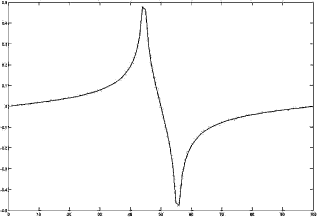
The result of computing the first derivative of a rect function in k-space. Due to the limited resolution (and the resulting low number of frequencies available), the result is not as clearly defined as its counterpart – the result of a numerical forward differentiation – in Figure 5.6.
Additional Tasks
In the LessonData-folder, you will find an improved version of FourierDiffRect_5.m named BetterFourierDiffRect_5.m. It does essentially the same but the outcome definitely resembles Figure 5.6 to a greater extent than Figure 5.35. Why?
5.4.7 Frequency filtering in Fourier-space on images
The script MouseFourierLP_5.m is derived from MouseSpectrum_5.m, and it implements a very simple low pass filter. In fact, all higher frequencies are cut off in a very rude manner, which leads to some artifacts in the resulting representation.
1:> img=zeros(733,733);
2:> img = imread(’MouseCT.jpg’);
3:> fimg = fft2(img);
Now, we remove the higher frequencies from the spectrum, and the result is displayed. Figure 5.36 shows the results when cutting off the frequencies for k > 5, k > 15, and k > 25; denote that the image in k-space is again shifted using fftshift in such a manner that the lowest frequency lies in the middle of the image. In order to implement a low-pass filter, we have to remove the frequencies whose absolute value is beyond a certain threshold. The lowest frequency is therefore found in the middle of the transformed image fimg, approximately at position (366, 366)T.
4:> fimg= fftshift(fimg);
5:> for i=1:733
6:> for j=1:733
7:> crad=sqrt((i-366)ˆ2+(j-366)ˆ2);
8:> if crad > 10
9:> fimg(i,j)=complex(0,0);
10:> end
11:> end
12:> end
13:> lpimg=zeros(733,733);
14:> lpimg = real(ifft2(fimg));
15:> minint=min(min(lpimg));
16:> lpimg=lpimg-minint;
17:> maxint=max(max(lpimg));
18:> lpimg=lpimg/maxint*64;
19:> colormap(gray);
20:> image(lpimg)

The output from script MouseFourierLP_5.m. Instead of smoothly suppressing higher frequencies like the Kblur kernel does, we simply cut off the frequencies, which leads to a lower image quality. A more sophisticated method would produce images just like Figure 5.3. Image data courtesy of C. Kuntner, AIT Seibersdorf, Austria.
Additional Tasks
Using the MouseFourierLP_5.m script, you can implement a simple high pass and band pass filter. A sample output can be found in Figure 5.37.
The basic operation in this script is actually the multiplication of the image in k-space with a function that is 1 in a circle of radius crad around the center of the image. Can you compute the PSF that would yield the same result by convolution in the spatial domain? A possible result can be found in Figure 5.38. Compare the image to Figure 5.31, and try to find some literature on Gibbs phenomenon.
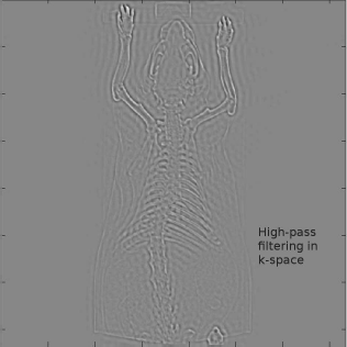
The results of a simple high pass filter in k-space applied to MouseCT.jpg. Image data courtesy of C. Kuntner, AIT Seibersdorf, Austria.

This PSF would give one of the blurred images from Figure 5.36. It can be derived by identifying the MTF in k-space and applying a Fourier-transform to it.
5.4.8 Applied convolution – PSF and the MTF
Finally, we will explore the full power of the convolution operation in k-space; the MouseConvolve_5.m script convolves a Gaussian with arbitrary standard deviation σ with the MouseCT.jpg image. Let’s take a look at the code. First, we read the image and transform it to k-space, and we allocate some space for a Gaussian named gs; the Gaussian is then drawn into the center of the image. sig defines the width σ of the Gaussian:
1:> img=zeros(733,733);
2:> img = imread(’MouseCT.jpg’);
3:> fimg = fft2(img);
4:> fimg = fftshift(fimg);
5:> gs=zeros(733,733);
6:> sig=2;
7:> for j=1:733
8:> for k=1:733
9:> gs(j,k)=exp(-((j-366)^2+(k-366)^2)/(2*sig^2));
10:> end
11:> end
The looks of the Gaussian can be found in Figure 5.39. Next, we transform the Gaussian to k-space - a step that is not necessary since a Gaussian stays a Gaussian when undergoing a Fourier-transformation5 - and we convolve the two functions by component-wise multiplication using the .* operator. The absolute value for the transformed Gaussian is also shown in Figure 5.39.
12:> gs=fftshift(fft2(gs));
13:> fimg=gs.*fimg;

The left image shows the Gaussian kernel gs with width σ = 2 in the spatial domain; this represents the PSF for the filtering process. The PSF is rather sharp and narrow; its counterpart in the Fourier-domain is the MTF. A well-defined PSF allows for good resolution of fine detail; therefore the MTF is wide. One may also notice that the MTF on the right hand side has also a Gaussian shape.
Next, we move back to the spatial domain; since our Gaussian was drawn in the center of the image to be convolved with MouseCT.jpg, we have to apply ifftshift twice. Finally, the image is scaled to 6 bit and displayed. The result of the operation using values σ ∈ {2,4, 6} is given in Figure 5.40.
14:> cimg=ifftshift(ifft2(ifftshift(fimg)));
15:> minint=min(min(cimg));
16:> cimg=cimg-minint;
17:> maxint=max(max(cimg));
18:> cimg=cimg/maxint*64;
19:> colormap(gray);
20:> image(real(cimg))
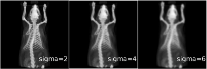
The results of the convolution operation with a Gaussian of width σ = 2, 4, and 6 pixels. Image data courtesy of C. Kuntner, AIT Seibersdorf, Austria.
Additional Tasks
Display gs in the spatial domain, and abs(gs) in k-space, similar to Figure 5.39. What happens for large values of sigma?
5.4.9 Determination of system resolution of an Anger-camera using a point source
By using a point source, it is possible to derive the MTF directly from an image. In this example, we have such an image of a point source. A syringe was filled with 99mTc and positioned over the scintillator crystal of a γ-camera. The camera allows to read out the image at various resolutions, ranging from 64× 64 to 1024 × 1024 pixels. The dimension of the scintillator is 614×614mm2. Two DICOM images named PSF64.dcm and PSF1024.dcm showing the needle tip can be found in your LessonData folder. The three subimages showing only the needle tip at the same scale can be found in Figure 5.41. The script ComputeMTF_5.m computes the MTF from these real life PSF images. Let us take a look at it. This version of the script reads the DICOM image taken with the lowest resolution of 64 × 64 pixels:
1:> clear;
2:> dimension=64;
3:> fp=fopen(’PSF64.dcm’,’r’);
4:> fseek(fp,-(dimension*dimension*2),’eof’);
5:> img=zeros(dimension,dimension);
6:> img(:)=fread(fp,(dimension*dimension*2),... ’uint16’);
7:> fclose(fp);

Two magnified images of a real life PSF in a γ camera. A syringe was filled with a small activity of 99mTc. These are the images of the needletip, all covering an area of 20×20 pixels, at two preset resolutions (64×64 and 1024×1024 pixels) of the γ camera. By computing the Fourier-transform of this PSF, it is possible to derive the overall system resolution of the γ camera. Image data courtesy of P. Schaffarich, University Clinic for Nuclear Medicine, Vienna General Hospital, Austria.
As usual, we clear all variables from our MATLAB-workspace, and since we are going to read the first image PSF64.dcm, which features a 64 × 64 matrix, we set the variable dimension to 64. Next, the file is opened, and we skip the DICOM header by simply starting 8192 bytes before the end of the file, denoted by the phrase ’eof’, which stands for end of file. Then we assign an empty matrix of 64 × 64 pixels, we read the image data into that matrix, and we close the file again.
8:> thresh = 300;
9:> weights=0;
10:> centroid=zeros(2,1);
11:> for i=1:dimension
12:> for j=1:dimension
13:> rho=img(i,j);
14:> if rho > thresh
15:> weights=weights+rho;
16:> centroid=centroid+rho*[i j]’;
17:> end
18:> end
19:> end
20:> centroid=round(centroid/weights);
21:> shift=[(centroid(1,1)-round(dimension/2))...
(centroid(2,1)-round(dimension/2))]’;
This part of the code is not directly connected to the determination of the system resolution. Rather than that, we determine the center of gravity of the image. Each pixel with an intensity above a certain threshold thresh is inspected. The pixel locations, which contain a gray value above 300 (denote that the intensity range is 0 ... 64555 since we are dealing with unsigned 16 bit images here, therefore everything below a gray value of 300 is considered plain black here), are added after scalar multiplication with their respective gray values, and the result is the center of mass of the image – in other words, we compute the weighted average of non-black pixels. The location of this center of mass is stored in a vector shift. More on the computation of centroids can be found in Chapter 6.
22:> cimg=zeros(dimension,dimension);
23:> for i=1:dimension
24:> for j=1:dimension
25:> rho=img(i,j);
26:> if rho > thresh
27:> if (i-shift(1,1) > 0) && ...
(i-shift(1,1) < dimension) && ...
(j-shift(2,1) > 0) && (j-shift(2,1) < dimension)
28:> cimg((i-shift(1,1)),(j-shift(2,1)))=img(i,j);
29:> end
30:> end
31:> end
32:> end
Here, we assign a new matrix for an image cimg, which is of the same dimension as img. The pixels are all shifted by the vector shift. The purpose of this procedure is to make sure that the most important part of the PSF, given by the center of mass of the image since it does not contain anything but the PSF, is located in the center of the image. Next, we can compute the Fourier-transform of cimg, which should give us the MTF. The absolute value of the Fourier-transform is computed, and we scale the intensities in the absolute values of the spectrum to a range of 0 ... 1:
33:> mtfimg = fft2(cimg);
34:> mtfimg=abs(fftshift(mtfimg));
35:> maxmtfimg=max(max(mtfimg));
36:> mtfimg=mtfimg/maxmtfimg;
Now we can derive a modulation transfer function plot like the one in Figure 5.21 from this image. Remember that we are only interested in the positive leg of the MTF, and that the MTF is radially symmetric since our PSF is also, at least in an idealized version, radially symmetric. Therefore, we simply save the intensities of the MTF in a line that is parallel to the x-axis of the image, and which starts in the middle of cimg:
37:> mtf=zeros(round(dimension/2),1);
38:> for i=1:round(dimension/2)
39:> mtf(i)=mtfimg(round(dimension/2),...
((round(dimension/2)-1) +i));
40:> end
41:> plot(mtf)
The result can be found in Figure 5.42. A matrix of 64 × 64 is pretty poor, and the result is not very impressive. The reason lies in the fact that the field-of-view is too small and limits the system resolution. Figure 5.43, which is connected to the Additional Tasks of this example, gives the MTF for a full resolution of 1024 × 1024 matrix.
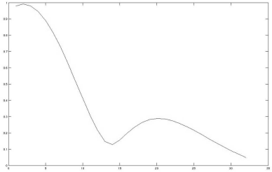
The result of ComputeMTF_5.m. We see a MTF for the PSF which is shown in the leftmost part of Figure 5.41. From this function it is evident that an Anger-camera with a field-of-view of 64 × 64 pixels can resolve up to 15 line pairs over the range of the scintillator – in general, it is said that a value of 0.1 still gives somes useful contrast. Since the width of the scintillator is 614 mm, 15 line pairs correspond to approximately 20 mm resolution.
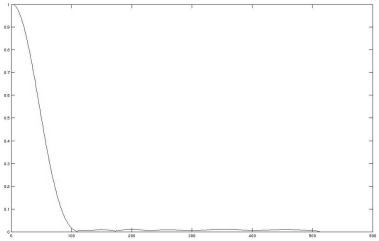
The result of ComputeMTF_5.m with the variable dimension set to 1024, and after reading in the file PSF1024.dcm. The resolution is no longer limited by the pixel resolution of the camera. The resolution in this diagram is given in “cycles over range” – therefore, 100 cycles over half the width of the scintillator results in a theoretical resolution of approximately 3 mm.
Additional Tasks
Check PSF128.dcm and PSF1024.dcm using ComputeMTF_5.m. Both can be found in the LessonData folder. Is the improvement in resolution dramatic, or is there some “void resolution” due to the fact that the ability to resolve fine detail is not only limited by the matrix of the digital image?
5.4.10 The Hough transform
In Hough_5.m, a Hough transform is carried out on the image shown in Figure 5.44. First, we read the image, and then we scale it to binary values – just to make sure that we have nothing but 0s and 1s in the image:
1:> img = imread(’evil.jpg’);
2:> minint=min(min(img));
3:> img=img-minint;
4:> maxint=max(max(img));
5:> img=round(img/maxint);

The binary image which will undergo a Hough-transform in Example 5.4.10. The representation in Hough-space can be found in Figure 5.46.
Next, we allocate an image for the Hough-representation named himg. It is 360 pixels wide (for all possible angles θ) and the maximum radius is given as 310×√2=439 (because size(img) = [310 310]). Just to make sure, we allocate 442 pixel for the radius r. If a nonzero pixel is encountered, we go through all angles θ, convert them in radians and derive the appropriate distance r = i cosθ + j sinθ. These parameter pairs increment the counts of found parameters on a trigonometric curve in himg. Take a closer look at the computation of r - in fact, we map all possible normal vectors to Hough space. This is also illustrated in Figure 5.45:
6:> himg=zeros(360,442);
7:> for i=1:310
8:> for j=1:310
9:> if img(i,j) > 0
10:> for ang=1:360
11:> theta=ang*pi/180;
12:> r=round(i*cos(theta)+j*sin(theta));
13:> if r > 0
14:> himg(ang,r)=himg(ang,r)+1;
15:> end
16:> end
17:> end
18:> end
19:> end

The basic principle of the Hough - transform is to store the parametric representation of the normal vectors →ni of lines that may pass a non-zero pixel p. If a series of pixels lies on a line, the location of the parameters for the normal vector of this very line will be densely populated. The parameters for less populated normal vectors are being disregarded prior to back-transformation.
Next, we have to reduce the number of parameters only to those spots in himg where most of the parameter pairs r, θ are found. This is done by thresholding the image (more on the subject can be found in Chapter 6). We introduce the threshold by a variable perc, which determines the percentage of the pixels below the maximum intensity maxint to be used. All pixels above that threshold are set to 64, all others are set to zero.
20:> perc=10;
21:> maxint=max(max(himg));
22:> for i=1:360
23:> for j=1:442
24:> if himg(i,j) > maxint-maxint*perc/100
25:> himg(i,j) = 64;
26:> else
27:> himg(i,j) = 0;
28:> end
29:> end
30:> end
By now, we already have everything, but the re-transformation from parameter space to lines is a little bit cumbersome. What follows is a lot of code, but it is not difficult to understand. For all remaining points {maxr, maxphi} in the thresholded parameter space, we compute the Hesse normal vector →n, named normalvect by transforming maxr and maxphi back to Cartesian coordinates. A second vector, unitvect, is computed as the normal vector to →n = (n1,n2) by setting its components to (-n2,n1). As one may easily verify from computing the inner product of this vector with →n, the two vectors are normal. Finally, the vectors length is scaled to 1.
31:> transimg=zeros(310,310);
32:> for maxphi=1:360
33:> for maxr=1:442;
34:> if himg(maxphi,maxr) > 0
35:> normalvect=zeros(1,2);
36:> unitvect=zeros(1,2);
37:> normalvect(1,1)=maxr*cos((maxphi)*pi/180) ;
38:> normalvect(1,2)=maxr*sin((maxphi)*pi/180) ;
39:> unitvect(1,1)=-normalvect(1,2) ;
40:> unitvect(1,2)=normalvect(1,1) ;
41:> unitvect=unitvect/(sqrt(unitvect(1,1)^2...
+unitvect(1,2)^2));
We have now a unit vector unitvect that gives the direction of the line defined by the Hesse normal vector normalvect. In order to draw a line, we have to move this unitvect to the tip of →n, and draw a pixel to the top of this shifted vector; after that, we increase the length len of unitvect, and draw the next pixel until we leave the domain of the image.
42:> len=0;
43:> i=round(normalvect(1,1)) ;
44:> j=round(normalvect(1,2)) ;
45:> while (i > 1) & (i < 309) & (j > 1) & (j < 309)
46:> i=round(normalvect(1,1)+len*unitvect(1,1)) ;
47:> j=round(normalvect(1,2)+len*unitvect(1,2)) ;
48:> transimg(i,j)=64;
49:> len=len+1;
50:> end
The same procedure is repeated, but the direction of unitvect is reversed. Finally, everything is displayed.
51:> unitvect=-unitvect;
52:> len=0;
53:> i=round(normalvect(1,1)) ;
54:> j=round(normalvect(1,2)) ;
55:> while (i > 1) & (i < 309) & (j > 1) & (j < 309)
56:> i=round(normalvect(1,1)+len*unitvect(1,1)) ;
57:> j=round(normalvect(1,2)+len*unitvect(1,2)) ;
58:> transimg(i,j)=64;
59:> len=len+1;
60:> end
61:> end
62:> end
63:> end
64:> colormap(gray)
65:> image(transimg)
Additional Tasks
In the LessonData folder, you may find a more medical example named MosaicBoneEdgeBinary.jpg, which is the result of Sobel filtering and intensity thresholding of an x-ray image of a long bone. Modify Hough_5.m in such a manner that this image is processed. By modifying perc, you will be able to display a number of straight lines in the image. Besides changing the intensity threshold of the image in Hough-space - can you think of a way to reduce the number of lines in the image transformed back to Cartesian coordinates? A small hint: think of the resolution of parameters in Hough space.
5.4.11 The distance transform
A simple little example illustrates the distance transform on the small binary rectangle from Figure 5.23, which also shows the result from the script DistanceMap_5.m. First, we load a 50 ×50 image of the rectangle, and we allocate some space for the transformed image. Next, we visit each pixel in the original image img. If such a pixel is not zero – remember that we are operating on binary images – we search for the nearest black pixel in the whole image. In order to find the correct distance, three conditions have to be met:
The nearest pixel in question has to be within the image domain.
It has to be zero.
And its distance must be smaller than the previously found distance; mindist is initialized as the maximum distance possible within the image. In the end, the smallest distance mindist is plotted in the image distImg and displayed as usual.
1:> img=imread(’dtrect.jpg’);
2:> distImg=zeros(50,50);
3:> for i=1:50
4:> for j=1:50
5:> mindist=71;
6:> if img(i,j)>0
7:> for k=-49:49
8:> for l=-49:49
9:> if (i+k)>0 && (i+k)<51 && (j+l)>0 && (j+l)<51
10:> if img((i+k),(j+l)) == 0
11:> dist=round(sqrt(k*k+l*l));
12:> if dist < mindist
13:> mindist=dist;
14:> end
15:> end
16:> end
17:> end
18:> end
19:> distImg(i,j)=mindist;
20:> end
21:> end
22:> end
23:> maxint=max(max(distImg));
24:> distImg=distImg/maxint*64;
25:> colormap(gray)
26:> image(distImg)
Until now, we have little use for this simple transformation; we will find it pretty useful later on. It should also be mentioned that we are not confined to the use of the Euclidean metric employed here, and that more effective (in terms of computing effort) implementations than the one presented here are feasible. However, for the moment, we can introduce one application of the distance transform, which is related to a morphological operation called thinning. Morphological operations are introduced in Section 6.6. We can make the result of Example 5.4.10 a little bit more impressive by computing the distance transform of Figure 5.47. After applying a distance transform we can apply a thresholding technique which we already encountered in Example 5.4.10, and which we will deal with in detail in Section 6.3. A more significant result is the effort of such an operation, which can be found in Figure 5.49.

An intermediate result of Hough_5.m. The binary image from Figure 5.44 is transformed to Hough-space; after thresholding the resulting image, only the areas with the highest concentration of parameter pairs remain. In this representation, the abscissa represents the angles θ, and the ordinate is the parameter r.

The final outcome of Hough_5.m. Using only the brightest 10% of the image, Figure 5.46 is transformed back to the line representation in Cartesian coordinates. Only the mouth of our slightly frustrated character remains. However, it is not limited to its original boundaries since the retransform from Hough space does not care whether we deal with line segments or lines. In Section 6.8.8.1, we will encounter the Hough transform again, and there we will learn how this problem can be handled.

The original x-ray image of a long bone, together with a ruler. This image is actually the result of mosaicing – it was assembled from several x-ray images acquired with a mobile x-ray unit. The lower image can also be found in the LessonData folder; a modification of Hough_5.m will produce an image similar to Figure 5.47. Image data courtesy of Z. Yaniv, ISIS Center, Department of Radiology, Georgetown University.
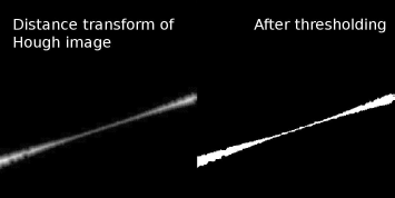
The distance transformation of Figure 5.47 and a binary version of that image after intensity thresholding. The centerline of Figure 5.47 is now emphasized.
Additional Tasks
Can you modify DistanceMap_5.m in such a manner that it produces something similar to Figure 5.49?
5.5 Summary and Further References
Filters and transformations are, as we have seen, two closely linked subjects. I admit that this chapter contains a lot of math, although I have only tried to motivate the use of separable transforms, namely the Fourier transform, in the complex domain. By no means can this short overview replace a solid background in applied and numerical mathematics. However, the importance of filtering operations justifies the effort since filtering is usually a vital component for other methods like segmentation, registration, and tomographic reconstruction. In this chapter, we have seen that the convolution operation, either in k-space or in the spatial domain can be arbitrarily combined in a linear manner to design more complex kernels. It is preferable to apply the convolution of more complex kernels in the Fourier-domain, and by means of the Fourier transform, we are also able to suppress periodic noise. Furthermore, we have learned about the PSF as a general tool for characterization of signal transmission in general, and how it is linked to the MTF. Finally, we made acquaintance with the Hough-transform, which allows to identify structures that are given in a parametric form.
Literature
R. C. Gonzalez, R. E. Woods: Digital Image Processing, Prentice-Hall, (2007)
M. Sonka, V. Hlavac, R. Boyle: Image Processing, Analysis, and Machine Vision, CL-Engineering, (2007).
W. Burger, M. J. Burge: Digital Image Processing – An Algorithmic Introduction using Java, Springer, (2008), http://www.imagingbook.com
1The law of refraction, also called Snell’s law, reads n1 sin θ1 = n2 sin θ2 where ni is the refractive index of the material that contains the ray, and θi is the angle of incidence associated.
2As for all kernels presented in this chapter, it is necessary to emphasize that we assume isotropic image data.
3Throughout this book, we use column vectors. However, for the sake of readability, we usually transpose such a column vector if it occurs within text; by doing so, we can write the vector as a row-vector.
4It is noteworthy that the terms eigenspace, eigenvector, and eigenfunction are not named after a person. It is a loan word from German; its direct translation would be something like own function. Eigenvectors and eigenfunctions span a sub-space – the eigenspace – of elements which are invariant to a given transformation. We will learn more about eigenvectors and eigenvalues in Chapter 7.
5Remember that the Gaussian retains its shape in k-space.