
Chapter 9
Registration
Wolfgang Birkfellner
9.1 Fusing Information
In Chapter 7, we dealt with all types of spatial transforms applicable to images. Besides visualization and interpolation purposes, these operations provide the core formalism for image registration or image fusion. From the very beginning of this book, it was emphasized that medical imaging modalities do not provide images of the patient’s anatomy and physiology. They do record certain physical properties of tissue. What sounds very philosophic is indeed a very general property of perception. We do only see what we can see – this forms our reality and our image of the world. But modern medical imaging devices enhance the limits of our perception. Less than forty years ago, the introduction of CT replaced invasive methods like exploratory laparotomy in case of unclear lower abdominal pain; MR gives stunning images of soft tissue where CT fails to achieve good image contrast. US allows for quick imaging not using ionizing radiation, and specialized probes allow even for using US inside the body. PET and SPECT visualize pathologies before these show up as anatomical changes by mapping metabolism and physiology. Still this plethora of information is worthless if it cannot be connected. This is mainly the task of well-trained experts in radiology, but the fact that most modern modalities produce 3D volume image data does not simplify the task of fusing information from different imaging sources. This is the domain of registration algorithms, where a common frame of reference for multiple data sources is established.
The main problem lies in the fact that the reference coordinate system of a volume dataset does not reference the patient – it references the scanner. Changing patient position between two imaging sessions is, however, necessary in many cases. The position of a patient in an MR scanner during a head scan is governed by the shape of the receiver coil and the gradients, whereas patient pose in a CT or PET scanner is governed by the patient’s principal axes. Combined modalities like PET/CT solve this problem; the poor anatomic image information from PET, especially in body regions other than the brain, renders exact fusion of PET and CT or MR difficult, and the information from the CT scan can even be used to improve volume reconstruction in the PET scan. Figure 9.1 gives a sample of the capabilities of a modern PET/CT system, and PET/MR systems are subject to clinical investigation. However, it is not that simple to combine modalities. A CT/MR scanner would be a very clumsy and difficult device, given the fact that the avoidance of ferromagnetic materials in the CT and the appropriate shielding of electromagnetic fields from the CT scanner is a rather delicate task. It would also be uneconomic to use such a system; a CT can handle more patients within a given period of time compared to an MR-tomograph.

An image sample from a combined PET/CT system. Registration of the PET and the CT volume is automatically achieved by taking both volume datasets in a scanner that is capable of recording both tracer concentration and x-ray attenuation. Image data courtesy of the Dept. of Nuclear Medicine, Medical University Vienna.
Fusion of images – that is, finding a common frame of reference for both images – is therefore a vital task for all kinds of diagnostic imaging. Besides fusing images for tasks such as comparison of image series, we can co-register the coordinate system of an external device such as a robot or a LINAC. It is also possible to merge abstract information, such as eloquent areas in the brain from a generalized atlas, to patient specific image information. In this chapter, we will introduce the most important methods and paradigms of registration. In general, all registration algorithms optimize parameters of rigid motion and internal dof (for deformable registration) until a measure that compares images is found to be optimal. The choice of this measure, which we will simply call merit function, depends on the specific registration task.
9.2 Registration Paradigms
In general, registration algorithms determine a volume transformation from identifying common features in two coordinate systems. These features can be intrinsic (that is features that are inherent to the image data) and extrinsic. Extrinsic features are usually markers attached to the patient; these markers, usually called fiducial markers, are identified in both frames of reference, but cause considerable additional clinical effort and are usually not available for retrospective studies. Registration algorithms can also be categorized by the type of image data or frames of reference they operate on. Let’s take a closer look at this classification.
9.2.1 Intra- and intermodal registration
In intramodal registration, we are registering images that stem from the same modality; an example is CT-to-CT registration of volumes acquired at different times. Such a procedure is extremely helpful when doing time series evaluation, for instance when tracking the effect of chemo- or radiotherapy on tumor growth. Here, a number of CT images is taken at different points in time. The one quantity of interest is tumor size, which can be identified easily provided a sufficient uptake of contrast agent. But with varying orientation of the patient, segmentation of the tumor and, above all, assessment of the direction of tumor growth or shrinkage becomes extremely cumbersome. By registration of the volumes, this task is greatly simplified since all slices can be viewed with the same orientation.
When fusing image data from different modalities, we are dealing with intermodal registration. A classical example is MR/CT fusion; an example of MR/CT fusion using an similarity measure named normalized mutual information (NMI) in AnalyzeAVW can be found in Figure 9.3. It is evident that different merit functions are necessary for this type of application. In intramodal registration, it may be sufficient to define a measure that compares the voxel gray values ρ at identical positions in the base and match volume. In intermodal registration, such an approach is bound to fail since the physical principle for the imaging modalities is different; therefore, there is no reason why a bright voxel in one volume should correspond to a bright voxel in the other volume. Our already well-known pig is actually the result of a series of experiments for multi-modal image registration. In total, the cadaver was scanned using T1, T2 and proton density sequences in MR as well as multislice CT and CBCT; after registration of those volumes, a single slice was selected and the images were blended. The result of this operation was stored as an MPG-movie. It can be found in the accompanying CD in the folder MultimediaMaterial under the name 7_MultimodalRegistration.mpg.
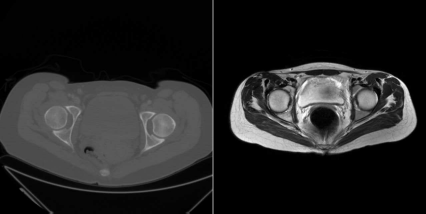
Two slices of the same patient at the same location, the hip joint. The left image shows the CT image, the right image is taken from the MR scan. Differences in the field-of-view and patient orientation are evident. Registration algorithms compensate for these discrepancies by finding a common frame of reference for both volume datasets. Image data courtesy of the Dept. of Radiology, Medical University Vienna.
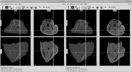
Two screenshots from the registration tool of AnalyzeAVW. On the left side, we see two slices of the MR and the CT scan, unregistered. Gross orientation is similar, but discrepancies are clearly visible. Besides soft tissue deformation, it is also evident that rigid structures such as the calvaria of the well-known pig scan do not coincide. After initiating the registration algorithm (in this case, an implementation of normalized mutual information), the two images match. The resulting volume transformation matrix V can be seen in Figure 9.4. Image data courtesy of the Dept. of Radiology, Medical University Vienna.
We will learn about specific merit functions in Section 9.3. Example 9.9.1 implements a very simple merit function computation for a rotated intramodal image; the merit function here is Pearson’s cross correlation coefficient, which we already know from Equation 7.16. Figure 9.21 shows the merit function for this very simple 2D-registration approach in one rotational dof.
9.2.2 Rigid and non-rigid registration
Rigid registration refers to algorithms that are confined to finding an affine transformation in three or six dof; affine transformations were extensively handled in Chapter 7. However, tissue may change its shape, and the relative position of inner organs may vary. Even the simple registration example shown in Figure 9.3 reveals this. In the registered transversal and coronal slices, we see that bony structures coincide very well. The soft tissue does not – this is simply due to the fact that the poor little piglet was decapitated before we scanned it. The head was sealed in a body bag, but in the case of the CT scan, it was lying in a plastic tub, whereas in the case of the MR, it was tucked into a head coil. The soft tissue was therefore deformed, and while the NMI-based registration algorithm of AnalyzeAVW does its job well (since it perfectly aligns the rigid anatomical structures), it cannot compensate for those deformations.
In non-rigid registration, the affine transformation is only a first step in alignment of volumes. The fine-tuning is handled by adding additional, internal dof, which handle the deformation as well. A non-rigid registration algorithm is therefore not a completely different approach to the registration problem; it relies on the same merit functions and optimization schemes, and it can be intra- or intermodal. What is added is actually a model that governs the deformation behavior. In other words, we need additional assumptions on how image elements are allowed to migrate. The formalism to describe this displacement is a deformation field. Each image element is displaced by a vector that indicates the direction and amount of displacement.
The distinctive feature for deformable registration methods is the way of modelling this displacement. In general, the mesh defining the displacement field is given, and local differences in the base and the match image are evaluated using a merit function; the local difference in the image define the amount of displacement for a single image element. The algorithms for modelling the displacement field can be put into the following categories:
Featurelet-based approaches: The most trivial approach is to sub-divide the image to smaller units, which are registered as rigid sub-units. The resulting gaps in the image are to be interpolated, similar to the volume-regularization approach mentioned in Section 7.2. This technique is also called piecewise rigid registration.
B-Spline-based approaches: In short, a spline is a numerical model for a smooth function given by a few pivot points. A mesh of pivot points is defined on the image, and the merit function chosen produces a force on the B-spline. The original meaning of the word spline is a thin piece of wood, used for instance in building the body of boats. Such a thin board will bulge if a force is applied to it, and its shape will be determined by the location of the pivot points – that is, the shape of the board under pressure depends on the location of its pivot points. It will be definitely different if its ends are clamped to a fixed position, or if they are allowed to move freely. The same thing happens to the B-spline. It can model deformation in a smooth manner, but huge local deformation will have a considerable effect on remote areas of the image.
Linear elastic models: For small deformations, it is permissible to treat the surface under deformation as an elastic solid. Local differences again apply a force on the elastic solid until an equilibrium is reached. The linearity assumption is only valid for small deformations, as one might know from real life. The advantage of this linear model, however, lies in the fact that non-local effects such as in the case of B-splines should not occur, but on the other hand, huge deformations cannot be compensated for.
Viscous fluid models: A generalization to the linear elastic model is the viscous fluid model, where strong local deformations are allowed; one can imagine a viscous fluid model as honey at different temperatures – it may be rather malleable or very liquid. Such a model allows for strong local deformations at the cost of registration failure if a large deformation occurs because of a flawed choice of internal parameters.
Finite-element models: In finite-element modelling (FEM), a complex mesh of the whole image is constructed, with well defined mechanical properties on interfaces of materials with different properties; in such a model, bone can be modelled as rigid, whereas other anatomical structures are handled as viscous fluids or as linear elastic models. The power of such an approach is evident since it models the structure of an organism. The drawback is the fact that a full segmentation of the volume of interest is necessary, and that constructing the mesh and solving the partial differential equations of a FE-model can be extremely labor- and time-intensive.
9.3 Merit Functions
In general, merit functions in registration provide a measure on the similarity of images; therefore, these functions are also referred to as similarity measures or cost functions. In general, these have the following properties:
They yield an optimum value if two images are aligned in an optimal manner; it is therefore evident that a merit function for intramodal registration may have completely different properties than an merit function for a special intermodal registration problem.
The capture (or convergence) range of the merit function should be as wide as possible. In other words, the merit function has to be capable of distinguishing images that are only slightly different from those that are completely different, and a well-defined gradient should exist for a range of motion as large as possible.
Merit functions for image fusion can be defined as intensity-based, or as gradient-based. The latter rely on differentiated images such as shown in Figure 7.21.
In general, merit functions assume a common frame of reference, and one of the two images “moves” by means of a volume transform; the merit function compares the gray values in the images at the same position in this common frame of reference. Figure 9.5 illustrates this concept.
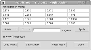
The volume transformation as produced by the AnalyzeAVW registration tool (see Figure 9.3).
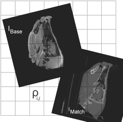
Merit functions compare gray values ρij in a common frame of reference. The images IMatch and IBase move in this common frame of reference, but the gray value is taken at the same location in the common coordinate system.
A number of intensity-based merit functions were defined, and most of them are basically statistical measures for giving a measure of mutual dependence between random variables. In these cases, the intensity values ρ are considered the random variables, which are inspected at the location of image elements which are assumed to be the same. This directly leads to a very straightforward and simple measure, the sum of squared differences:
MSSD=1N*N∑(ρBase(x,y,z)−ρMatch(x,y,z))2 (9.1)
where N is the total number of pixels. The inner mechanics of this measure are evident; if two gray values ρ differ, the squared difference will be non-zero, and the larger the difference for all image elements, the larger the sum of all squared differences will be. It is evident that this measure will work best for completely identical images with the same histogram content, which only differ by a spatial transform. A more versatile merit function can be defined by using Equation 7.16; in this case, the correlation coefficient of paired gray values ρBase(x, y, z) and ρMatch(x, y, z) is computed. Pearson’s cross-correlation assumes a linear relationship between the paired variables, it does not assume these to be identical. This is a clear progress over MSSD given in Equation 9.1. Still it is confined by definition to intramodal registration problems. And, to add some more real life problems, one can usually not assume that the gray values ρ in two intramodal images follow a linear relationship. Nevertheless, a merit function MCC can be pretty useful sometimes, and a sample implementation is given in Example 9.9.1.
Another possibility to compare intramodal images is to take a look at the difference image Idiff of two images, and to assess the disorder in the result. Such a measure is pattern intensity, given here only for the 2D case:
MPI=N∑x,y∑d2≤r2σ2σ2+(Idiff(x,y)−Idiff(u,v))2d=(x−u)2+(y−v)2σ=Internal scaling factor (9.2)
d is the diameter of the local surrounding of each pixel; if this surrounding is rather homogeneous, a good match is assumed. This measure, which has gained some popularity in 2D/3D registration (see Section 9.7.2), assesses the local difference in image gray values of the difference image Idiff within a radius r, thus giving a robust estimate on how chaotic the difference image looks like. It is very robust, but also requires an excellent match of image histogram content; furthermore, it features a narrow convergence range and therefore can only be used if one is already pretty close to the final registration result. The internal scaling factor σ is mainly used to control the gradient provided by MPI.
So far, all merit functions were only suitable for intramodal registration (and many more exist). A merit function that has gained wide popularity due to the fact that it can be applied to both inter- and intramodal registration problems is mutual information.1 This measure from information theory gives a measure for the statistical dependence of two random variables which is derived from a probability density function (PDF) rather than the actual gray values ρ given in two images. This sounds rather theoretic, but in practice, this paradigm is extremely powerful. The PDF - we will see later on how it can be obtained - does not care whether a voxel is tinted bright, dark or purple; it just measures how many voxels carry a similar value. Therefore, a PDF function can be derived for each image, and the mutual information measure is defined by comparing these functions in dependence of a registration transformation. In general information theory, mutual information (MI) is defined as:
MI=E(P(IBase,IMatch))ln P(IBase,IMatch)P(IBase)P(IMatch) (9.3)
where E (P (IBase,IMatch)) is the expectation value of the joint PDF - noted as P (IBase,IMatch) in Equation 9.3 - of the two images IBase and IMatch, and P(IBase) and P (IMatch) are the PDF for the gray values in the single images. So far, this definition is not very useful as long as we do not know what the expectation value of a PDF is, and how the single and joint PDFs are derived. So what exactly is a PDF? A PDF is a function that gives the probability to encounter a random variable x in sampling space. For a random variable that follows the normal distribution, the PDF is given as the Gaussian. For an image, a nice approximation of a PDF is the histogram, which we already know from Section 4.3.
The joint histogram is a 2D function that maps from a 2D-domain, namely the gray values of the images IBase and IMatch, to a statistic that measures the occurrence of a similar gray value at the same pixel (or voxel). Note that the gray values need not be the same; the basic idea of mutual information lies in the fact that areas with similar content will have a similar distribution of gray values. If we define a measure that becomes optimal if the joint histogram is as well-organized as possible, we can assume an optimum match of the images IMatch and IBase. Ex. 9.9.2 computes the joint histogram for an image and itself (where the disorder in the joint histogram is minimal), and the same image after slight rotation and translation. Figure 9.6 shows the result.
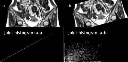
The output from the JointHistogram_9.m script in Example 9.9.2. In the upper row, we see two MR images, which can be found in the LessonData folder and are named OrthoMR (a) and OrthoMRTransf (b). They are the same images, but they differ by a small rotation and translation. The lower images show the output of the JointHistogram_9.m script in Example 9.9.2 – first, the joint histogram of image a and itself is computed (lower left). We see a low level of disorder in the histogram since all gray values are well correlated and aligned nicely on the line of identity in the joint histogram. The joint histogram of images a and b look worse; the common occurrence of similar gray values is scarce, and the cells with high counts in the histogram are more scattered (lower right). Disorder – measured by Shannon’s entropy – is higher here. The surface plots of these joint histograms can be found in Figure 9.8. Image data courtesy of the Dept. of Radiology, Medical University Vienna.
In order illustrate the idea of a joint histogram, we can introduce it also with a simple example from statistics; let us consider a group of people. Among those, four are girls and five are boys. Furthermore, three of them are milk drinkers, and the other six prefer beer. The histogram for this distribution is to be found in Figure 9.7.
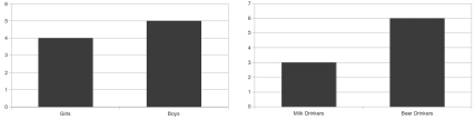
A statistical example for illustrating the joint histogram. Out of a group of nine people, four are female. Furthermore, three group members prefer non-alcoholic beverages. A joint histogram of this statistical collective is given in Table 9.1.
Now let us take a look at the joint histogram of this group. Such a joint distribution is the well-known 2× 2 table, shown in Table 9.1. Later in this chapter, we will return to this table and illustrate the concept of entropy using this example.
The 2 × 2 table for our simple example of girls and boys, drinking beer or milk. The central part of this table is a joint histogram of the two properties, similar to the Figures 9.6, 9.8 and 9.9. Later in this chapter, we will illustrate the concept of “disorder” (or entropy) using this example.
Girls |
Boys |
Total |
|
|---|---|---|---|
Milk drinkers |
2 |
1 |
3 |
Beer drinkers |
2 |
4 |
6 |
Total |
4 |
5 |
9 |
Back to images. Figure 9.6 shows an ideal case for a joint histogram. In an intramodal image with similar gray values, the optimal joint histogram becomes a straight line; if we would compute the correlation coefficient according to Equation 7.16, we would get a value of 1 since the joint histogram can be considered a scatterplot in this case – it is not exactly scatterplot since a scatterplot does not weight common values of ρ within a given bin higher. If all values align nicely along a line, Pearson’s correlation coefficient yields an optimum value. Therefore, we could ask ourselves why MCC should be any worse than a MI-based merit function MMI. The answer is easily given when taking a look at Figure 9.9. Here, an MR and a CT slice from a co-registered dataset were rotated against each other; if the rotation angle is 0°, the match is optimal. The associated joint histogram, however, does not align to a straight line. This is not surprising since the functional relationship between MRI- and CT-gray values is neither linear, and it is not even monotonous. The mutual information measure can nevertheless assess the disorder in the joint histogram, just as the correlation coefficient does in the case of a linear relationship in a scatterplot.
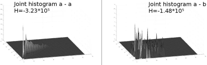
Surface plots of the joint histograms given in Figure 9.6. The first histogram – which is the joint histogram of the MR image a from Figure 9.6 with itself – shows that the histograms are not scatterplots. Rather than that, different bins show different heights. The second surface plot shows the joint histogram of the MR image and its rotated counterpart (image b from Figure 9.6). Apparently, more bins are non-zero, but the overall height is much lower – note that the z-axes have a different scale. The bin height ranges from 0 to 350 in the left plot, whereas the bin height in the right plot does not exceed 4. Shannon’s entropy as given in Equation 9.4 was also computed for both histograms. It is considerably lower for the well-ordered left histogram, as expected.
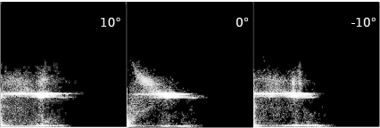
The joint histogram of two registered slices from the LessonData folder, CT.jpg and T1.jpg. The images were rotated against each other with an angle of -10°, 0°, and 10°; while the joint histogram for the optimum case (rotation angle 0°, middle image) does not look like the lower left image in Figure 9.6, since the images are taken from different modalities, it is optimal in terms of disorder, as one can see when computing the mutual information as a merit function. A series of joint histograms for this multimodal case can be found in Example 9.9.2 when running MultimodalJointHistogram_9.m.
In Figure 9.9, we see that there is a subtle change in the appearance of the joint histogram; since we only apply a rotation, we always have a rather large overlapping area. If we perform a translation, the number of densely populated areas does obviously change to a greater extent, with large sparsely populated areas. A script that performs such a trans-lation for the CT- and MR-datasets named MultimodalJointHistogramTranslation_9.m can be found in the LessonData-folder. The joint histograms for overlap and translations in y-direction of -100 and 100 pixels can be found in Figure 9.10.

Another example for the joint histogram of two registered slices from the LessonData folder, CT.jpg and T1.jpg. This time, one of the slices was translated by -100 pixels, and by 100 pixels. Since the overlap of the images is less than in the case of image rotation (see Figure 9.9), the disorder in the joint histogram is increased, resulting in visibly less densely populated areas in the joint histogram. Again, a series of joint histograms for this multimodal case can be found in Example 9.9.2 when running MultimodalJointHistogramTranslation_9.m.
We see that a well-ordered histogram is characterized by the fact that most points in the joint histograms are accumulated in a few areas. This is independent of the range of gray values - a scaling operations would just stretch the joint histogram, or it would move the densely populated areas to other positions in the joint histogram. A measure for this disorder in a PDF P, which we will call entropy2 from now on, is Shannon’s entropy:
H=−∑iPiln (Pi) (9.4)
Without expanding in mathematical detail, it is evident why Equation 9.4 is a good measure for entropy (or disorder, as we called it previously). A joint histogram with densely populated bright areas (that is, bins with a high count of occurrences) show a lesser degree of chaos than a sparsely populated joint histogram with a “dark” appearance. A high count – that is a bright spot in the joint histogram – increases H, but the logarithm – a function that grows at a very slow rate for higher values, as we have seen in Example 4.5.3 – as a second factor defining the elements of H suppresses this growth very effectively. Furthermore, the sum of counts in two joint histograms of high and low entropy should be the same. As a consequence, the histogram with low entropy has only a few non-zero elements, and the high value of Pi is damped by the term ln(Pi). The chaotic histogram, on the other hand, has many summands with a low value Pi and this value is not damped by the logarithmic term.
Our simple example given in Figure 9.7 and Table 9.1 might help to understand this concept. For the sample of beer- and milk-drinking boys and girls, we can also compute Shannon’s entropy:
H=−(2ln (2)+ln (1)+2ln (2)+4ln (4))=−8.317 (9.5)
A possible joint distribution with lesser entropy would be the following – all girls drink beer and some boys drink milk or beer. The total numbers have not changed – we still have the same number of males and females, and the number of milk or beer drinkers also stays the same. Therefore, we have the following joint histogra Computing Shannon’s entropy gives the following result when neglecting non-populated cells in the joint histogram since ln(0) = −∞:
H=−(3ln (3)+4ln ()+2ln (2))=−10.227 (9.6)
The Entropy in this case is obviously lower than the one given in Equation 9.5, which was derived from the distribution in Table 9.2 despite the fact that the total numbers are the same. The reason for this lies in the fact that - if one knows one property of a random person from our sample - one can make more likely conclusions about the other property. If we encounter a girl from our group, we do know that she prefers beer. This is order in a statistical sense. The same holds true for our joint histograms of images - in a well registered image, we can conclude the gray value in the match image from the gray value in the base image, no matter what their actual value is.
An alternative 2 × 2 table for beer- or milk-drinking girls and boys. While the total numbers stay the same, this distribution shows lesser disorder since we can make quite likely conclusions about the other property from a given property.
Girls |
Boys |
Total |
|
|---|---|---|---|
Milk drinkers |
0 |
3 |
3 |
Beer drinkers |
4 |
2 |
6 |
Total |
4 |
5 |
9 |
Equation 9.4 also lies at the very foundation of (MMI), the mutual information merit function; while Equation 9.4 by itself is already a fine merit function, the related formulation of a mutual-information merit function based on Equation 9.3 has become popular. We define a merit function that utilizes mutual information as follows:
MMI=H(IBase)+H(IMatch)−H(IBase,IMatch) (9.7)
Without expanding on joint entropy, Shannon entropy, Kullback-Leibler distances3 and more information about theoretical measures, we may simply believe that Equation 9.7 is a measure for the common information in two images, which is optimal if the two images are aligned.
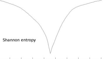
The Shannon entropy for the joint histogram as computed in Multimodal-JointHistogram_9.m in Example 9.9.2. The abscissa shows the angle of relative rotation of the T1.jpg and CT.jpg from the LessonData folder, which ranges from -90° to 90°. Again, an optimum is encountered when the two images match at a relative rotation of 0°. The corresponding joint histogram is shown in the middle of Figure 9.9.
The true power of MMI lies in the fact that it does not care about gray values; it retrieves all information from the PDF, which is basically given by the histogram. Therefore, it is a truly multimodal merit function. In Example 9.9.3 we plot the cross-section for the 3D merit function MMI when rotating and translating the T1.jpg and CT.jpg slices. The shape of the merit function can be found in Figure 9.12. Many more refinements of merit functions for multimodal image registration exist, for instance it is possible to derive the PDF using the so called Parzen-window method. The basic idea - minimization of entropy in a joint PDF of the images - however, always stays the same. For the sake of completeness, we should also add the definition of a variation of MMI called normalized mutual information:
MNMI=H(IBase)+H(IMatch)H(IBase,IMatch). (9.8)

The output from the script PlotMutualInformation2D 9.m in Example 9.9.3. The shape of MMI is plotted when changing all three dof of rigid motion in 2D separately for the two sample images T1.jpg and CT.jpg. Despite the fact that this representation is ideal and that a clear maximum of MMI can be seen, local optima are visible and may cause a failure of the registration procedure.
Multimodal matching always necessitates that the gray value ρ in corresponding image elements is replaced by a more general measure; the joint entropy in PDFs derived from images is one possibility. Another possibility is the use of gradient information in an image; if we recall the edge-detection mechanisms as presented in Chapter 5 and Example 7.6.6, we see that the edge image itself retains only very little information on gray levels; one can even segment the filtered edge-image, so that only a map of ridge lines remains. Figure 9.14 illustrates this operation on our already well-known pig slices CT. jpg (the base image) and T1. jpg (the match image) from Figure 9.23.

A more complex clinical example of multimodal image registration. Here, a PET and an MR scan of a sarcoma in the pelvis was registered. Since PET provides very little anatomic information, a direct registration of MR and PET data in the abdominal area often fails. However, it is possible to register the MR data with the CT data that came with the PET-scan from a PET-CT scanner using normalized mutual information; in this case, the implementation of AnalyzeAVW was used. The registration matrix obtained is applied to the PET data since these are provided in the same frame of reference as the CT data. Image data courtesy of the Dept. of Radiology and the Dept. of Nuclear Medicine, Medical University Vienna.
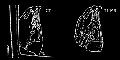
CT.jpg and T1.jpg after Sobel-filtering, optimization of image depth and thresholding. After this process, the differences in gray values in the two images disappear, and only gradient information remains. Applying a gradient-based measure to such an image allows for multi-modal image registration without computing joint histograms or using an intensity based measure.
As we can see from Figure 9.14, the differences in image intensities usually do not interfere with the delineation of edges (with some exceptions, like the additional edges in MR that stem from the better soft-tissue contrast). If we can design a merit function based on these gradient images, we may have another merit function for multimodal image fusion at hand. Such a measure is chamfer matching; it uses a binary image for IMatch that was made using a Sobel filter and intensity thresholding such as shown in Figure 9.14, and a distance transform (see Section 5.3.2) of IBase that was processed in the same manner. Figure 9.15 shows the distance transform of T1.jpg after differentiation and intensity thresholding.
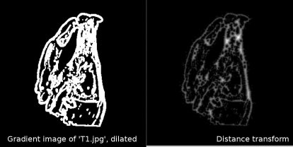
T1.jpg after Sobel-filtering, intensity thresholding, and dilation (left). This image can be found in the LessonData folder as T1_EdgeImageDilated.jpg. The right image shows its distance transform (DT_ChamferMatch.jpg in LessonData). The image is an intermediate result of Example 9.9.4. In the chamfer-matching algorithm, the sum of the entries in the distance transform of IBase at the location of non-zero pixels in IMatch is computed while IMatch moves over the base image.
The chamfer matching merit function MCM is simply defined as:
MCM=∑x,yD(IBase(x,y))x,y...Pixels in IMatch with ρ*0D(IBase)...Distance transform of IBase (9.9)
Equation 9.9 can be understood as follows; D (IBase) - the distance transform from Section 5.3.2 - defines grooves in the binary gradient image IBase, and if IMatch “drops” into those grooves, MCM becomes optimal. A plot of MCM is computed in Example 9.9.4. This merit function has a severe drawback – it only works well if we are already close to the solution of the registration problem. Another example of such a merit function is Equation 9.3. In Section 9.4, we will discuss this problem to a further extent.
Finally, we can also compare images by employing an orthonormal series expansion, of which we heard in Chapter 5. Remember that every coefficient in such an expansion is unique; if we compare corresponding coefficients of the same order, we can compare images. If we compare the norms of the components in a Fourier transform, we are able to decouple translation and rotation since translation is only a complex phase in the Fourier-domain. The norm of a complex number does not know about complex phases, and therefore such a merit function would be translation-invariant. However, merit functions based on series expansions tend to be computationally expensive, and by nature, they are confined to binary or strictly intramodal image data. But if we would like to solve the registration problem when facing a merit function as shown in Figure 9.9, it might be a viable way to solve the rotation problem first and finding an optimum translation afterwards.
Here ends our presentation of merit functions; many more exist, and some of them provide valuable additional tools in our arsenal for specialized tasks. However, we have learned about the basic types of the most important methods for comparing images. What we have not yet dealt with is the question of finding an optimum in the merit function, rather than presenting functions that exhibit a known optimal value.
9.4 Optimization Strategies
The plots from Figs. 9.6, 9.9, 9.10, 9.11, 9.12 and 9.16 all presented a somewhat misleading idea of the general shape of a merit function. Here, only one dof was varied, whereas the others were kept constant at the correct value. Furthermore, we only deal with rather harmless images showing the same region of our object, and all images were in 2D. If we switch to 3D, we end up with merit functions that are dependent on six parameters (for instance three quaternions - the fourth one is defined by the requirement that the quaternions are normalized - and three dof in translation). The graphical representation of a function M (Δx,Δy,Δz,q1,q2,q3) = r, where r is a real-valued scalar is nevertheless a considerable task. It is even more difficult to find an optimum in a six-dimensional valley. This is the task of an optimization algorithm.

The results of Example 9.9.4; this is a plot of the chamfer matching merit function in 3 dof through the solution of the registration problem. The plots can be directly compared to Figure 9.12, derived in Example 9.9.3. As we can see, numerous local minima exist and for translation, there is no wide gradient. Therefore it is necessary to start the optimization algorithm close to the expected solution, since otherwise, finding the minimum is unlikely.
The optimization problem can be imagined as a salad bowl and a marble. If we have a nice, smooth salad bowl and a nice, smooth marble, the marble can be released at any point and it will find its way to the minimum under the influence of gravity. Nature always does so, and an Irish physicist, W. R. Hamilton, even made that a general principle, the principle of least action. Another creation of Sir William Rowan Hamilton we have already encountered - he has also opened our eyes to the world of quaternions.
In our less than perfect world, we may however encounter problems in optimization. Our salad bowl may be a masterpiece of design, shaped like a steep cone with a very small opening (like a champagne glass), whereas we have to use a football in order to solve this problem because of a sudden shortage of marbles. The principle of least action is still valid, but we will not see the football roll to the deepest point of the salad bowl. Other salad bowls may have a very rough and sticky surface, and our marbles may be small and our marble could be badly damaged because of being a veteran of fierce marbling contests in the past. The salad bowl is the merit function, and the marble is the optimization algorithm, grossly speaking. I will not further expand on the problems of n-dimensional salad bowls.
Optimization algorithms can be categorized as local and global algorithms. The problem with all optimization algorithms is that they can fail. Usually, the algorithm starts at a given position and tries to follow the gradient of the merit function until it reaches an optimum. Note that we do not care whether we face a maximum or a minimum, since every merit function showing a maximum can be turned over by multiplying it with -1. Since the merit function is only given on discrete pivot points, we have no chance of knowing whether this optimum is the absolute optimum (the optimal value the merit function reaches over its domain), or if there is another hidden optimum. The mathematical counterpart of the saladbowl/marble allegory is the simplex algorithm, also called Nelder-Mead method. Here, the marble is replaced by a simplex, which can be considered an n-dimensional triangle. If our simplex is one-dimensional and is supposed to find the minimum of a simple one-dimensional function f(x) = y, it is a segment of a straight line; this simplex crawls down the function f(x), and its stepwidth is governed by the gradient of f(x). Once the simplex encounters a minimum, it reduces its stepwidth until it collapses to a point. Figure 9.17 illustrates this algorithm in a humble fashion.
![Figure showing a simple illustration of the Nelder-Mead or simplex algorithm, a local optimization algorithm; a simplex in one dimension is a section of straight line that follows the gradient of a function; as the simplex approaches a minimum, [inline] is true, and the simplex makes smaller steps until it collapses to a point since the gradient to the right is ascending again and the algorithm terminates. It cannot find the global minimum to the right, but it is stuck in the local minimum.](http://imgdetail.ebookreading.net/software_development/2/9781466555594/9781466555594__applied-medical-image__9781466555594__image__009x314.png)
A simple illustration of the Nelder-Mead or simplex algorithm, a local optimization algorithm; a simplex in one dimension is a section of straight line that follows the gradient of a function; as the simplex approaches a minimum, ddxf(x)≃0
The simplex-algorithm is one of many optimization methods; other algorithms like Powell’s method, Levenberg-Marquardt, conjugate gradient and so on are well-documented in numerous textbooks. All these algorithms are local optimizers - they are good at finding the obvious nearest minimum, and some of them require the computation of derivative functions, whereas others do not. The simplex is of special interest for us since it is incorporated in MATLAB® as fminsearch, and Example 9.9.5 demonstrates it.
Global optimizers try to tackle the problem of finding - as the name implies - global optima. The simplest type of a global optimization method is a full search in the parameter space with decreasing stepwidth. Imagine you have a set of N starting parameters ∇p
9.5 Some General Comments
Registration, despite the considerable complexity of a full-featured implementation of a high-performance registration tool, is the more pleasant part of medical image processing compared to segmentation. After all, MMI is a measure that works as a good basic approach for many registration problems. Therefore it would be reasonable to use mutual information, combined with global optimizers and maybe a deformation model for coping with non-rigid deformations, for all registration problems.
In real life, this does not work. While mutual information is an excellent measure, it also sacrifices information by omitting the actual gray values from the images after forming the PDF; if the joint histogram is sparsely populated, for instance due to lacking information in one of the images, the measure is likely to fail. An example is MR/PET registration, one of the first applications for this measure in neuroscience. Fusing MR and PET images of the brain works well since a high and specific uptake of tracer yields lot of information. If one tries to accomplish the same with PET images of the body, the difficulties are considerable. This has led to the development of PET/CT, and PET/MR is a further development under research for the time being.
If a combined scan is not feasible, it may be a good idea to resort to registration techniques using external markers (see also Section 9.7.1). Another problem related to sparse histogram population, which results in an inconclusive optimum for the Shannon entropy, is often encountered in 2D/3D registration (see Section 9.7.2), where six dof of motion in 3D are retrieved from planar images. Therefore one is well advised to consider alternatives, especially when dealing with intramodal registration problems, to improve the robustness of the registration algorithm by utilizing more stringent merit functions.
Another challenge lies in the evaluation of registration algorithms; we will encounter the well-accepted measures of target registration error (TRE) and fiducial registration error (FRE) in Section 9.8. However, it is also interesting to explore the reliability of an implementation, which is not only dependent on the merit function used, but also on the clinical application area, the imaging modalities used, and the configuration of the optimization algorithm used; a validation of a registration algorithm can, for most practical purposes, only be carried out by repeated runs of the algorithm with randomly changing starting positions, which may be confined to different maximal values. And it should take place on as many datasets as available.
Another problem that is ignored pretty often lies in the fact that we are optimizing for parameters which are given in different units. Rotations are given in radians or degrees, and translations are given in voxels, pixels, or millimeters. The optimization algorithm scales itself to the function slope, but it is not necessarily aware that a change in 1° in rotation may have a way more dramatic effect on the image compared to a translation of 1 pixel.
So what can be done to achieve good registration results? Here is a small checklist:
Initialization: As we can see in Example 9.9.5, it is advisable to start the registration close to expected solution; one may, for instance, position the volumes or images manually. Or it is possible to move the volumes to the same center of gravity – a principal axes transform may also help to obtain an initial guess for the relative rotation of the images.
Appropriate choice of the merit function: The nature of the registration problem governs the choice of the merit function. In general, one may consider other statistical measures than mutual information if a intramodal registration problem is given. Gradient based methods tend to have a smaller capture range than intensity–based methods.
Appropriate choice of optimization methods: Global optimizers tend to require lots of computational time while a correct result is not guaranteed. One may try a good implementation of a local algorithm first. Sometimes, a multiscale approach is proposed. Here, the volumes are scaled down and the registration problem is handled on this coarse stage first before proceeding to finer resolution. This approach is, however, not always successful – it may as well lead to local optima and considerable runtime.
Avoid additional degrees-of-freedom: It is of course possible to match images of different scale using an additional scaling transformation, and of course one could always try to carry out a deformable registration in order to avoid errors from changing soft tissue. Don’t do this – additional dof increase the risk of winding up in local optima.
Restriction to relevant image content: This is an often underestimated aspect. It is very helpful to constrain the area in IBase used for merit function validation. This does not only refer to the spatial domain, but also to intensities. A lower bound in intensity can, for instance, improve robustness by suppressing noise and structures that stem from the imaging modality such as the table in CT. And it can be helpful to exclude parts of the body which moved relative to each other; an example is the registration of abdominal scans such as shown in Figure 9.2, where it is advisable to exclude the femora since these are mobile relative to the pelvis.
9.6 Camera Calibration
Another important technique, especially for image-guided therapy (Section 7.5) and visualization (Chapter 8) is the determination of projection parameters of a 3D body to a 2D imaging plane. The shape of the projection image will, of course, be determined by the actual pose of the 3D body, which can be described by an affine rigid body transformation in homogeneous coordinates, and by the position of the projection source and the projection screen relative to the 3D-body. In Chapter 8, we have learned how to produce such projected images from 3D datasets. In camera calibration, the inverse problem is being treated - how can we determine both the 3D-position of an object and the properties of the camera - that is, any projection system including x-ray machines and head-mounted displays - from the projected image? In the most simple (and common) of all cases, we just want to know about the reference coordinate system and the distance of the focal spot (or the eyepoint) of our camera; this can be determined by projecting single points with a known 3D-position onto a projection screen (which can be an x-ray image detector or a display as well). Figure 9.18 illustrates this problem.
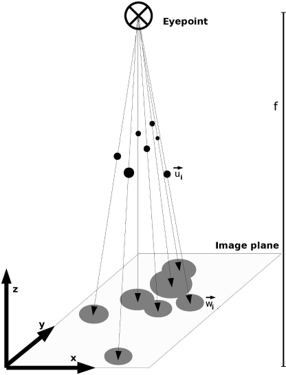
An illustration of the camera calibration problem. In this example, the imaging plane is located in the x-y plane of a Cartesian coordinate system. The normal distance of the eyepoint - the source of projection - is located at a distance f from the imaging plane. The known coordinates of the fiducial markers →ui are projected onto the plane, and their coordinates are given as →wi. The task is to determine f and an affine transformation that locates the eyepoint in the coordinate system.
In order to tackle the camera calibration problem, we have to remember another matrix, which is the projector P. In mathematics, each matrix that fulfills the requirement P = P2is called a projection. Let’s go to Figure 9.18 - the effect of P→ui is the 2D image of the markers. If we project this image again, nothing will change. A projection matrix that maps 3D positions →ui to 2D positions →wi to the x-y plane of a Cartesian coordinate system where the eyepoint is located at the the z-axis at a distance f is given as:
P=(10000100000000−1f1) (9.10)
One can easily verify that P is a projector indeed. The projector operates on a point i£ by multiplication. If we want to apply the volume transformation V on that point prior to projection, we have to compute [inline]. You may remember that, in order to change the position of the eyepoint by another volume transformation [inline], we have to compute [inline]. Since we deal with a projection in homogeneous coordinates here, we have to add a rescaling step to w′ to get coordinates w - remember that the fourth element of vector giving homogeneous coordinates has to be 1, which is not the case when applying an operator like P.
In the camera calibration problem, we know a set of N planar projected coordinates →wi∈{→w0...→wN} and the associated 3D coordinates →ui∈{→u0...→uN}. We have to find out about V and f. A simple algorithm to achieve this is called the Direct Linear Transform (DLT). It is easily formulated using homogeneous coordinates; a 3D coordinate →u is transformed by a 4 × 4 matrix PV = D, where P is given in Equation 9.10 and V is our well-known affine transformation matrix from Section 7.3.2, as:
D→u=→v (9.11)
It is, however, necessary to renormalize the resulting vector →v by computing →w=→vv4. We omit the z-variable since it is of no importance for the projected screen coordinates; therefore we have a resulting pair of screen coordinates:
→w′=(w1w201) (9.12)
All we have to find out is the twelve components of matrix D; by expanding the matrix product and using Equation 9.12 we can rewrite Equation 9.11 as:
D11u1+D12u2+D13u3+D14=w1*v4 (9.13)
D21u1+D22u2+D23u3+D24=w2*v4 (9.14)
D41u1+D42u2+D43u3+D44=v4 (9.15)
We can insert Equation 9.15 in Eqs. 9.13 and 9.14, which gives us two equations with twelve unknowns D11, D12, D13, D14, D21, D22, D23, D24, D41, D42, D43, and D44. These can be rewritten as a 12 × 2 matrix:
(u1u2u310000−w1u1−w1u2−w1u3−w10000u1u2u31−w2u1−w2u2−w2u3−w2)(D11D12D13D14D21D22D23D24D41D42D43D44)=→0 (9.16)
where →0 is a vector containing zeros only. If we have at least six points →ui, we can augment the matrix from Equation 9.16 by adding more rows; let us call this matrix S and the vector containing the components of matrix D is called →d. Equation 9.16 becomes a homogeneous system of equations S→d=0, which can be solved using, for instance, a linear least squares method. Example 9.9.6 demonstrates this. A number of more sophisticated variations of this algorithm exist; these can also compensate for distortions in the projection images such as the radial distortion in wide angle optics, or for the higher order distortion encountered in analog image intensifies used in C-arms. But, at least for the calibration of modern amorphous silicon x-ray imaging detectors, the DLT is usually fine.
9.7 Registration to Physical Space
So far, we have talked about image-fusion; we have learned that we can merge images of the same origin and from different modalities, and that we can enhance the affine transformation in six dof by adding internal dof of deformation, which is governed by various models. But in a number of applications (remember Section 7.5), it is necessary to map a coordinate system defined in physical space to an image coordinate system. Application examples include the registration of a patient, whose coordinate system is defined by a rigidly attached tracker probe, to an MR or CT-volume. Another example includes the registration of a robot’s internal frame-of-reference to a patient, who is either fixated by molds or other devices, or who is tracked as well. In the following sections, a few techniques for registration to physical space will be introduced.
9.7.1 Rigid registration using fiducial markers and surfaces
Until now, we have dealt with intensity based registration; if intensity based algorithms fail, one may resort to explicit landmarks, which can either be prominent anatomical features, or explicitly attached so-called fiducial markers. This is an extremely important technique, not only in image processing, but also in image-guided therapy, where a match between patient and image data is to be achieved. Figure 9.19 shows the so-called Vogele-Bale-Hohner mouthpiece, a non-invasive device for registration using fiducial markers. The mouthpiece is attached to the patient by means of a personalized mold of the maxillary denture. A vacuum pump evacuates the mold, therefore the mouthpiece is held in position in a very exact manner. The strength of this setup is certainly fusion of anatomical image data and SPECT or PET datasets, where an intensity-based algorithm often fails due to a lack of common information in the images.
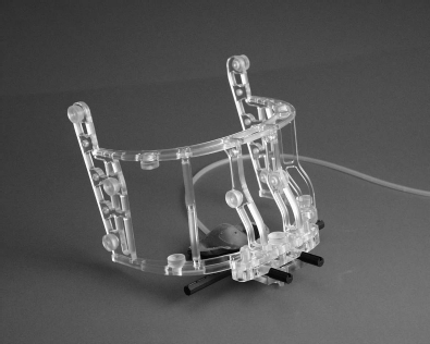
The Vogele-Bale-Hohner mouthpiece, a device for non-invasive registration using fiducial markers. The mouthpiece is personalized by means of a dental mold. A vacuum pump ensures optimum fit of the mouthpiece during imaging. Image courtesy of Reto Bale, MD, University Clinic for Radiology University of Innsbruck, Austria.
In the best of all cases, the coordinates of the markers match each other. If the transformation matrix is composed as a rotation followed by a translation (V = TR) one can immediately determine three dof of translation by computing the centroid of the marker pairs according to Equation 6.1 in both frames of reference. The difference of the two cen-troids gives the translation vector. After translation of the marker positions so that the centroids of the point pairs {→p1,→p2,...→pN} and {→p′1,→p′2,...→p′N} match, a rotation matrix R that merges the positions best can be determined if the markers are not collinear - in other words, the points must not lie on a line. And we do need at least three of them. Let PBase be the set of coordinates in the base reference frame, and P'Match be the matching set of points in the coordinate system to be registered after they were translated to the centroid. This can, however, also be done inside the algorithm. In this setup, the center of rotation is the centroid of the base point set.
One of the most widely used algorithms for matching ordered point sets was given by Horn.4 It matches two ordered point sets PBase and PMatch by minimizing
M=12N∑i=1||→pBasei−V→pmatchi||2 (9.17)
where V is the well-known affine volume transformation matrix. After computing the centroids →ˉpBase and →ˉpMatch, one can define a 4 × 4 covariance matrix C of the point sets as
C=1NN∑i=1(→pMatchi−→pMatch)(→pBasei−→pBase) (9.18)
Next, an anti-symmetric matrix A = C - CT is formed from C; the vector Δ is given by Δ = (A23, A31, A12)T. Using this vector, one can define a 4 × 4 matrix Q:
Q=(trCΔTΔC+CT−trCI3) (9.19)
tr C is the trace of matrix C, the sum of all diagonal elements. I3 is the 3 × 3 identity matrix. If we compute the eigenvectors and eigenvalues of Q and select the eigenvector that belongs to the biggest eigenvalue, we have four quaternions. A rotation matrix R can be derived by using Equation 7.19. These are the parameters of the optimum rotation that match the point sets. The translation is derived, as already mentioned before, by computing:
→t=1NN∑i=1→pMatchi−R→pBasei (9.20)
Example 9.9.7 implements such a computation.
A logical next step would be to enhance the method to non-ordered point sets. This is for instance important if one wants to match surfaces, which are digitized and given as node points. Matching two such meshes is a widespread problem, for instance in image-guided therapy. If one segments a body surface from a CT- or MR-scan, it is possible to generate a mesh of the resulting surface (as presented in Chapter 8), consisting of node points. Another modality such as a surface scanner, which produces a 3D surface by scanning an object using optical technologies for instance, can produce another mesh of the patient surface in the operating room. Surface data can also be collected, for instance, by tracked ultrasound probes, where a 3D point is assigned to a 2D point in the US-image by tracking the scanhead using some sort of position measurement device (see Section 7.5). By matching the surface as scanned and the segmented surface, it is possible to achieve a match of the patients position in the treatment suite to the volume image; in such a case, the node points of the meshes are matched by using a point-to-point registration technique, but the point sets are not ordered.
An enhancement of the method as presented in Eq. 9.18, Eq. 9.19 and Eq. 9.20 is the so-called iterative closest point (ICP) algorithm, which was presented in the already mentioned paper by P. Besl and N. McKay. In the ICP-algorithm, the distance d between a single point →p and a surface S is defined as d(→p,S)=min →x∈S||→x−→p||. Computing such a minimum distance is not new to us - we have done this before in Example 6.8.7. The result of this search for closest points is an ordered set of corresponding points from S which are closest to the points →p in our matching surface, which is given as a set of points →p. What follows is a point-to-point registration as shown before. The next step is to repeat the procedure, with a new set of closest points as the results. This procedure can be repeated until a termination criterion is met - usually this is the minimal distance between closest points.
The ICP-algorithm, which had numerous predecessors and refinements, also lies at the base of surface-based registration algorithms. If one tries to match two intramodal datasets, a feasible way is to segment surfaces in both volumes is to segment these surfaces, create a mesh, and apply an ICP-type of algorithm. This is generally referred to as surface registration; it is, however, usually inferior to intensity-based algorithms such as mutual information measure based methods. First, it requires segmentation, which can be tedious; second, the ICP algorithm is sensitive to outliers. A single errant node point, generated by a segmentation artifact for instance, can screw up the whole procedure.
9.7.2 2D/3D registration
Registration of the patient to image data is not confined to point- or surface-based methods; it can also be achieved by comparing image data taken during or prior to an intervention with pre-interventional data. An example of such an algorithm is the registration of a patient to a CT-dataset using x-ray data. If one knows the imaging geometry of an x-ray device, for instance by employing a camera-calibration technique (see Section 9.6), If the exact position of the x-ray tube focus is known relative to the patient (for instance by using a tracker, or from the internal encoders of an imaging device), one can derive six dof of rigid motion by varying the six parameters for the registration transformation. The fact that x-ray is a central projection with a perspective (which is governed by parameter f in Equation 9.10) is of the utmost importance in this context since a motion to and from the x-ray tube focus changes the scale of the projection. In a 2D/3D registration algorithm, DRRs are produced iteratively, and a merit function is used to compare the DRR to the actual x-ray image. Once an optimum match is achieved, the registration parameters are stored and give the optimum transform. This type of registration algorithm is usually more complex and sometimes tedious compared to 3D/3D registration since the optimization problem is not well defined. Multimodal and non-rigid 2D/3D registration are also open challenges.
Figures 9.20 shows a reference x-ray, a DRR before registration and the overlay of the two. In the folder MultimediaMaterial, you will also find a MPG-movie named 7_2D_3DRegistration.mpg which shows a 2D/3D registration algorithm at work.5 The movie shows the series of DRRs and the merit function; after convergence, an overlay of the DRR and the reference x-ray is displayed.

Three images of a spine reference-dataset for 2D/3D image registration. We see the reference x-ray on the left, the DRR generated from the initial guess, and the registration result. An edge image of the x-ray is overlaid over the final DRR after 2D/3D registration.
9.8 Evaluation of Registration Results
As usual in medical image processing, many algorithms can be defined, but they tend to be worthless if a substantial benefit for clinical applications cannot be shown. Therefore, evaluation is a crucial problem here. The most important measure for registration is, of course, the accuracy of the registration method. Such a measure was introduced initially for image-guided therapy, but it also fits general registration problems perfectly well. It is the target registration error (TRE).6 In image fusion, points (that must not be the fiducial markers in the case of marker based registration) randomly chosen from the base volume are transformed to the match volume (or vice versa), and the average or maximal Euclidean distance of the two positions in the base and match coordinate system is computed. It is however important to sample more than one point, and to distribute them evenly over the whole volume.
In image-guided therapy, the issue is a little bit more complex. Here, a fiducial marker has to be localized in patient space by means of a tracker or a similar device, which has an intrinsic error. This initial localization error is called fiducial localization error (FLE). The FLE does of course affect the precision of a marker-based registration method. After computing the registration transform from the marker positions, the euclidean distance between the markers in the target volume and their transformed positions is given by the fiducial registration error (FRE), which is sometimes reported by a IGT-software suite as a measure for the quality of the registration. This measure is, however, misleading. If the original distribution of markers is positioned in a more or less collinear manner, the quality of the registration may, for instance, be pathetic despite an excellent FRE. It is therefore also necessary to determine a TRE in addition to the FRE; since the localization of a target is usually carried out by a tracker, the tracker accuracy may affect TRE as well.
Besides accuracy, it is also necessary to report the range of convergence for a measure; this can be done by a random sampling of starting points within a certain initial TRE, and a comparison of resulting TREs. A report on failed registrations (where the algorithm does not converge or produces a result worse than the initial TRE) and on algorithm runtimes is also mandatory. Finally, a validation should be carried out on phantom datasets which allow for determination of a ground truth such as our pig-dataset we tormented to such a large extent in this chapter. It is actually from such a dataset since it carries multimodal fiducial markers.
9.9 Practical Lessons
9.9.1 Registration of 2D images using cross-correlation
CC2DRegistration_9.m is a script derived from Example 7.6.1. In this example, we rotate a single 2D image by an angle φ ϵ {-90° ... 90°} and compute Pearson’s cross-correlation coefficient given in Equation 7.16 as a merit function. The values for the merit function in dependence of the rotation angle are stored in a vector ccvals. The single MR-slice of our already well-known pig head (see also Figure 7.12) is loaded and a matrix rotimg is allocated for the rotated image. Furthermore, the vector ccvals is declared:
1:> img=imread(’PorkyPig.jpg’) ;
2:> rotimg=zeros(300,300);
3:> ccvals=zeros(181,1) ;
Next, we enter a loop where the rotation angle φ is varied from -90° to 90° in 1° steps. The rotation matrix is defined. We perform a nearest neighbor interpolation by transforming the new coordinates newpix in rotimg back to the original image img. Furthermore, we also rotate the image around its center, therefore the center of the image is transformed to the origin of the coordinate system by a vector shift; after rotation, the coordinates are shifted back. The result is a rotated image such as shown in Figure 7.14 from Example 7.6.2.
4:> for angle=-90:90
5:> rotmat=zeros(2,2);
6:> rotmat(1,1)=cos(angle*pi/180);
7:> rotmat(1,2)=-sin(angle*pi/180);
8:> rotmat(2,1)=sin(angle*pi/180);
9:> rotmat(2,2)=cos(angle*pi/180);
10 :> invrotmat=transpose(rotmat);
11:> oldpix=zeros(2,1);
12:> newpix=zeros(2,1) ;
13:> shift=transpose([150,150]) ;
14:> for i=1:300
15:> for j=1:300
16:> newpix(1,1)=i;
17:> newpix(2,1)=j;
18:> oldpix=round((invrotmat*(newpix-shift))+shift);
19:> if (oldpix(1,1) > 0) & (oldpix(1,1) < 300) & (oldpix(2,1) > 0) & (oldpix(2,1) < 300)
20:> rotimg(i,j)=img(oldpix(1,1),oldpix(2,1));
21:> end
22:> end
23:> end
Next, we compute the correlation coefficient; since we are only interested in the optimum of this simple merit function, we do not care about normalization factors and so on. Furthermore, the merit function becomes maximal for an optimum match; it is therefore inverted by displaying its negative value. Finally, the contents of the merit function vector ccvals are displayed. We store the result of the merit function evaluation in an array ccvals. Since we change the angle of rotation from -90 to 90°, we have to add 91 to the variable angle for proper indexing. A plot of ccvals can be found in Figure 9.21.

The output of Example 9.9.1. When rotating the image from Figure 7.12 from -90° to 90° and computing the correlation coefficient as given in Equation 7.16, we get an optimum correlation if the two images match; this is, of course, the case for a rotation of 0°. A registration algorithm computes the spatial transform to match two images by optimizing all dof until a minimum in the merit function is found.
24:> meanImg=mean(mean(img));
25:> meanRotImg=mean(mean(rotimg));
26:> ccdenom=0.0;
27:> ccnomImg=0.0;
28:> ccnomRotImg=0;
29:> for i=1:300 30:> for j=1:300
31:> ccdenom=ccdenom+double(((img(i,j)-meanImg)* (rotimg(i,j)-meanRotImg)));
32:> ccnomImg=ccnomImg+double(((img(i,j)-meanImg)^2));
33:> ccnomRotImg=ccnomRotImg+double(((rotimg(i,j)-meanRotImg)^2));
34:> end 35:> end
36:> ccvals((angle+91),1)=-ccdenom/ (sqrt(ccnomImg)*sqrt(ccnomRotImg));
37:> end 38:> plot(ccvals)
In a full-fledged implementation of a registration algorithm, a minimum for all three dof would be computed by an optimization algorithm, thus producing the parameters for a registration matrix V .
Additional Tasks
Implement a translation rather than a rotation, and inspect the result.
Implement intramodal merit functions other than cross correlation from Section 9.3.
A modified script, More2DRegistration_9.m compares two registered slices of the porcine phantom taken with different types of CT; the first one is a slice from the already well-known multislice CT dataset, the other one was taken using a CBCT machine attached to a linear accelerator. While this is an intramodal image registration problem, the imaging characteristics of the two machines are different concerning dose, dynamic range of the detector, and tube voltage. Inspect the results for the intramodal merit functions in this script. Two examples for MSSD and MCC are given in Figure 9.22.
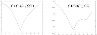
Two sample outputs from modified versions of More2DRegistration_9.m, where two registered slices of a CBCT and a CT were rotated against each other, and the result was evaluated using Equation 9.1, the sum of squared differences, and MCC – the merit function based on Pearson’s cross correlation coefficient. While MSSD performs fine (left side), MCC exhibits an local minimum at approximately 140° that may even lead to a failure in a registration process.
9.9.2 Computing joint histograms
In JointHistogram_9.m, we compute the joint histogram for an MR image of a female pelvis. The images can be found in the LessonData folder as OrthoMR and OrthoMRTransf. They are stored as DICOM-images since the greater depth helps to make the result of joint histogram computation more evident. First, we load the two images img and rimg, and we allocate a matrix that holds the joint histogram jhist:
1:> fp=fopen(’OrthoMR’,’r’);
2:> fseek(fp,2164,’bof’);
3:> img=zeros(380,160);
4:> img(:)=fread(fp,(380*160),’short’);
5:> fclose(fp);
6:> fp=fopen(’OrthoMRTransf’,’r’);
7:> fseek(fp,960,’bof’);
8:> rimg=zeros(380,160);
9:> rimg(:)=fread(fp,(380*160),’short’);
10:> fclose(fp);
11:> jhist=zeros(900,900);
Next, we compute the joint histogram of img with itself; each pixel location (i, j)T is visited, and a scatterplot of the gray values rho1 and rho2 is produced. Since our indices in jhist start with one rather than zero, we increment rho1 and rho2 by one for easier indexing. The joint histogram jhist gives the statistics of occurrence in this scatterplot. In order to improve the visibility of the gray values in the joint histogram, we compute the logarithm of jhist, just as we did in Example 4.5.3. After inspecting the result, we are prompted to proceed:
12:> for i=1:380
13:> for j=1:160
14:> rho1=img(i,j)+1;
15:> rho2=img(i,j)+1;
16:> jhist(rho1,rho2)=jhist(rho1,rho2)+1;
17:> end
18:> end
19:> jhist=log(jhist);
20:> maxint=double(max(max(jhist)));
21:> jhist=jhist/maxint*255;
22:> colormap(gray)
23:> image(jhist)
  24:> foo=input(’Press RETURN to advance to the joint histogram of the different images...
’);
Now, the same procedure is carried out using img and rimg. The result can be found in Figure 9.6.
25:> jhist=zeros(900,900);
26:> for i=1:380 27:> for j=1:160
28:> rho1=img(i,j)+1 ;
29:> rho2=rimg(i,j)+1 ;
30:> jhist(rho1,rho2)=jhist(rho1,rho2)+1 ;
31:> end
32:> end
33:> jhist=log(jhist);
34:> maxint=double(max(max(jhist))) ;
35:> jhist=jhist/maxint*255;
36:> colormap(gray)
37:> image(jhist)
Additional Tasks
MultimodalJointHistogram_9.m is a combination of JointHistogram_9.m and More2DRegistration_9.m. It displays the joint histogram for CT.jpg and T1.jpg when rotating the images against each other with an angle of ϕ ϵ {90°...90°} with steps of 10°. Run the script and inspect the result (see also Figure 9.9). In addition, compute joint entropy according to Equation 9.4 for in the script and plot it. The output should look similar to Figure 9.11.
MultimodalJointHistogramTranslation_9.m is essentially the same script as MultimodalJointHistogram_9.m, but it does not perform a rotation but a trans-lation in y-direction by an amount [inline] pixels by a stepwidth of 10 pixels. The overlapping area of the two images is smaller in this case, and the differences in the joint histogram are more evident. Figure 9.10 shows some of the results.
9.9.3 Plotting the mutual information merit function
PlotMutualInformation2D_9.m, is directly derived from More2DRegistration_9.m and MultimodalJointHistogramTranslation_9.m. It computes the cross-section of the merit function MMI through the known optimal registration in all three dof of rigid motion in 2D; for the sake of brevity, we only take a look at the part where the MMI is computed; the remainder is basically identical to the scripts from Example 9.9.2. First, a vector mi is defined, which holds the values for the merit function; then, the histograms and joint histograms are derived:
...:> mi=zeros(37,1);
...
...:> jhist=zeros(256,256);
...:> histImg=zeros(256,1);
...:> histRotimg=zeros(256,1);
...:> for i=1:388
...:> for j=1:388
...:> rho1=img(i,j)+1;
...:> rho2=rotimg(i,j)+1;
...:> jhist(rho1,rho2)=jhist(rho1,rho2)+1;
...:> histImg(rho1)=histImg(rho1)+1;
...:> histRotimg(rho2)=histRotimg(rho2)+1;
...:> end
...:> end
The histograms are derived for each step in translation; basically speaking, this is not necessary since the histogram of the base image does not change. It is done here nevertheless to keep the code compact. Next, we compute Shannon’s entropy for the histograms of img and rotimg, which are in fact the PDFs P(IBase) and P(IMatch) from Equation 9.7. MMI is computed and stored in the vector mi. We elegantly circumvent the problem that ln(0) = -∞ by computing H (which is named shannon. . . in the script) only for non-zero values:
...:> shannonBase=0;
...:> shannonMatch=0;
...:> shannonJoint=0;
...:> for i=1:256
...:> for j=1:256
...:> if jhist(i,j) > 0
...:> shannonJoint=shannonJoint+jhist(i,j)* log(jhist(i,j));
...:> end
...:> end
...:> if histImg(i) > 0
...:> shannonBase=shannonBase+histImg(i)* log(histImg(i));
...:> end
...:> if histRotimg(i) > 0
...:> shannonMatch=shannonMatch+histRotimg(i)* log(histRotimg(i));
...:> end
...:> end
...:> shannonBase=-shannonBase;
...:> shannonMatch=-shannonMatch;
...:> shannonJoint=-shannonJoint;
...:> mi((a+19),1)=shannonBase+shannonMatch-shannonJoint;
Figures 9.12 shows the output for the three movements, which all cross the optimum position in the middle.
Additional Tasks
Implement Equation 9.8 and compare the outcome.
9.9.4 Chamfer matching
For matching the thresholded gradient images of CT.jpg and T1.jpg, we need a distance transform of IBase, which is computed by the script DTChamfermatch_9.m. This script is directly derived from DistanceMap_4.m from Example 5.4.11 and will therefore not be discussed here. Since the inefficient implementation of the distance transform in DistanceMap_4.m causes a long runtime, we have also stored the result as DT_ChamferMatch.jpg in the LessonData folder. The base image derived from T1.jpg and its distance transform can be found in Figure 9.15. The actual chamfer matching merit function is computed in PlotChamferMatch2D_9.m, which is derived from PlotMutualIn-formation2D 9.m. Again, we only comment on the changes in the script compared to its predecessor; first, we read the distance transform image DT ChamferMatch.jpg, which is our base image. The image that undergoes the transformation is called otherimg - this is the thresholded gradient image CT EdgeImage.jpg. An array for the resulting chamfer matching merit function MCM named cf is also allocated:
...:> img=double(imread(’DT_ChamferMatch.jpg’)) ;
...:> otherimg=double(imread(’CT_EdgeImage. jpg’)) ;
...:> rotimg=zeros(388,388);
...:> cf=zeros(37,1);
Next, the image undergoes a rotation by an angle [inline] by steps of 10°. The resulting image is rotimg. The merit function MCM is computed and stored in cf :
...: > sumInt=0;
...:> for i=1: 388
...:> for j=1: 388
...:> if rotimg(i, j)>0
...:> sumInt = sumInt+img(i,j) ;
...:> end
...:> end
...:> end
...:> cf((a+19),1)=-sumInt;
In short words, the value of the distance transform is summed up at the location of a non-zero pixel in rotimg, which is our IMatch. The same procedure is repeated for translation in x- and y-direction. The resulting values for MCM are found in Figure 9.16. It is evident that MCM will only provide useful registration results if the optimization procedure starts close to the solution since significant local minima and lacking gradients at a larger distance from the correct result will make optimization a very difficult task.
Additional Tasks
Develop a more efficient version of DTChamfermatch 9.m by replacing the euclidean metric by a so-called Manhattan metric; here, only the shortest distances in x- and y- direction are sought and plotted. Usually, a distance transform derived using the Manhattan-metric is sufficient for chamfer matching.
Improve the convergence radius of MCM by dilating T1 EdgeImage-Dilated.jpg to a larger extent prior to computing DT ChamferMatch.jpg using DTChamfermatch -7.m. You may use the dilation filter of GIMP or the script from Example 6.8.6. Why should this help?
9.9.5 Optimization
First, we want to explore the properties and pitfalls of numerical optimization. For this purpose, we define two very simple one-dimensional functions that can be found in Figure 9.24. One is a sine, overlaid with a spike-type function producing a number of local minima and one global minimum. We will try to find out whether the MATLAB-implementation of the simplex algorithm is able to find the global minimum in dependence of its starting point. The other function is a simple spike, showing one global minimum but virtually no gradient – and we will observe what happens in such a case.

Three sample slices from co-registered volumes; T1.jpg is taken from an MR-volume, whereas CT.jpg and CBCT.jpg are from CT-volumes. The images are used in Examples 9.9.1, 9.9.2 and 9.9.3.

The functions defined in the scripts strangeSine.m and spike.m. Both show somewhat unpleasant properties; the first one features a series of local minima, the other has a gradient of zero for most of its domain.
In the SimpleOptimization_9.m7 example, we apply a simplex algorithm to two functions, defined in separate scripts strangeSine.m and spike.m.
As said before, we have abdicated from many of MATLAB’s advanced functions for the sake of simplicity; we have not used vector notation whenever possible (at the cost of performance), we have not used the graphical user interface (GUI) functionality of MATLAB, and we have not used functions. The latter becomes necessary now since the MATLAB-function fminsearch utilizes function pointers. A MATLAB-function is defined in a separate script that is named like the function. A function that takes three input variables x, y and z and returns a vector with two components is defined by the following syntax:
function [resOne, resTwo] = myFunction(x,y,z)
...
resOne = ...
resTwo = ...
end
where one may do whatever he wants with x, y, and z. The first of the two functions to be optimized in this example is defined in the script strangeSine.m and is defined as follows:
1:> function [sSine]=strangeSine(x)
2:> sSi=sin(x)+3;
3:> if x > 10.8 && x < 11.2
4:> sSi=sSi-1;
5:> end
6:> sSine=sSi;
7:> end
This is a sine with a somewhat strange global minimum at x=72π≃10.99557. The other function is defined in spike.m. It is a narrow inverse rect-function:
1:> function [spi]=spike(x)
2:> sp=1;
3:> if x > 4.95 && x < 5.05
4:> sp=0;
5 :> end
6:> spi=sp;
7 :> end
This function is zero for all values of the independent variable [inline], and one otherwise.
The script SimpleOptimization 9.m minimizes the two functions in dependence of a starting value xs using the function fminsearch. First, the function is plotted in a vector minvect over a range of approximately 7.2π or 1300°. The result is found in Figure 9.24, together with a plot of spike.m. Next, the minimum for the function is sought using fminsearch. The function strangeSine.m is referenced using the @-operator; this is actually a pointer to the function strangeSine.m, so that the fminsearch-routine can call it independently. A starting point xs is provided in ascending order from 1 to 20 radians. If the starting point is close to the location of the global minimum x = 10.99557, it gives the correct solution. Otherwise, it converges to a local minimum. The found minima are plotted as a function of xs in Figure 9.25. The option ’.’ causes plot to show single bullets instead of a connected line.
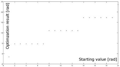
The optimization result of strangeSine.m in dependence of the starting value xr. Only for a limited range, the correct value (which is approximately 11) is found, otherwise the optimizer is struck in local minima.
1:> mfunct=zeros(1300,1);
2:> for xs = 1:1300
3:> mfunct(xs) = strangeSine(xs*pi/180.0);
4:> end
5:> plot(mfunct)
6:> foo = input(’Press RETURN to see the minima found by the simplex...’);
7:> minxvect=zeros(20,1);
8:> for xr = 1:20
9:> minxvect(xr)=fminsearch(@strangeSine,xr)
10:> end
11:> plot(minxvect,’.’)
12:> foo = input(’Press RETURN to see the next function...’);
An interesting effect shows up when running the script using Octave instead of MAT-LAB; at least in my current version, it appears as if the implementation of the Nelder-Mead algorithm is inferior to the one in MATLAB. Octave only finds one correct minimum, very close to the solution, and fails otherwise. The output from SimpleOptimization_9.m in Octave can be found in Figure 9.26. I therefore apologize to Octave users, who may encounter severe problems with this example.
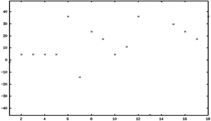
The result of optimizing strangeSine.m using the implementation of the simplex algorithm of Octave. It should look exactly like Figure 9.25. However, the internal settings of the optimizer cause a very poor convergence behavior.
The same procedure is repeated for spike.m.
13:> mfunct=zeros(1000,1);
14:> for xs = 1:1000
15:> mfunct(xs) = spike(xs/100.0);
16:> end
17:> plot(mfunct)
18:> foo = input(’Press RETURN to see the minima found by the simplex...’);
19:> minxvect=zeros(1000,1);
20:> for xs = 1:1000
21:> minxvect(xs)=fminsearch(@strangeSine,(xs/100));
22:> end
23:> plot(minxvect)
Again, the correct minimum (which is any value between 4.95 and 5.05) is only found if the starting value is close enough to the true solution of the optimization problem (see Figure 9.27).
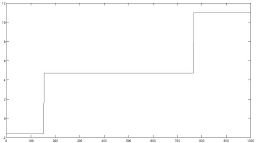
The result for the optimization of the inverse rect-function spike.m; the starting values xs range from 0 to 10 in steps of 0.01. Only if the starting value is close enough to the solution, the correct minimum (approximately 5) is found.
So far, these are very simple functions; we can apply the same procedure to functions of more than one variable. This can be done for instance by modifying PlotMutualInfor-mation2D_9.m from Example 9.9.3. Let us take a look at the function to be optimized; we still stick to planar 2D slices (if you have not already guessed about their nature, you may take a short look at Figure 9.23).
The merit function to be optimized takes three arguments provided in a vector start. This is the angle of rotation around the image center, and the translation in 2D. The script defining the merit function is MI2D.m. Note how the transform is carried out; first, the pixel position is shifted to the image center. Next, it is rotated, and shifted back to a corner of the image. Finally, the translation is applied. The order of transformations is T R. MI2D.m is not carried out by you in MATLAB – rather than that, it is called from a second script named Optimize2D_9.m, which will be introduced soon:
1:> function [mf] = MI2D(start)
2:> baseimg=imread(’CT.jpg’);
3:> matchimg=imread(’T1.jpg’);
4:> rotimg=zeros(388,388);
5:> rotmat=zeros(2,2);
6:> rotmat(1,1)=cos(start(1,1)*pi/180);
7:> rotmat(1,2)=-sin(start(1,1)*pi/180);
8:> rotmat(2,1)=sin(start(1,1)*pi/180);
9:> rotmat(2,2)=cos(start(1,1)*pi/180);
10:> invrotmat=transpose(rotmat);
11:> oldpix=zeros(2,1);
12:> newpix=zeros(2,1);
13:> shift=transpose([194,194]);
14:> tshift=transpose([(start(2,1)),(start(3,1))]);
15:> for i=1:388
16:> for j=1:388
17:> newpix(1,1)=i;
18:> newpix(2,1)=j;
19:> oldpix=round(((invrotmat*(newpix-shift))+shift)+ tshift);
20:> if (oldpix(1,1) > 0) && (oldpix(1,1) < 388) && (oldpix(2,1) > 0) && (oldpix(2,1) < 388)
21:> rotimg(i,j)=matchimg(oldpix(1,1),oldpix(2,1));
22:> end
23:> end
24:> end
The mutual information merit function is implemented in the same manner as in Example 9.9.3. An important difference lies in the fact that fminsearch searches for a minimum, whereas the mutual information as defined in Equation 9.7 becomes a maximum; we simply invert the merit function by multiplying it with -1.
25:> jhist=zeros(256,256);
26:> histImg=zeros(256,1);
27:> histRotimg=zeros(256,1);
28:> for i=1:388
29:> for j=1:388
30:> rho1=baseimg(i,j)+1;
31:> rho2=rotimg(i,j)+1;
32:> jhist(rho1,rho2)=jhist(rho1,rho2)+1;
33:> histImg(rho1)=histImg(rho1)+1;
34:> histRotimg(rho2)=histRotimg(rho2)+1;
35:> end
36:> end
37:> shannonBase=0;
38:> shannonMatch=0;
39:> shannonJoint=0;
40:> for i=1:256
41:> for j=1:256
42:> if jhist(i,j) > 0
43:> shannonJoint=shannonJoint+jhist(i,j)* log(jhist(i,j));
44:> end
45:> end
46:> if histImg(i) > 0
47:> shannonBase=shannonBase+histImg(i)* log(histImg(i));
48:> end
49:> if histRotimg(i) > 0
50:> shannonMatch=shannonMatch+histRotimg(i)* log(histRotimg(i));
52:> end
53:> end
54:> shannonBase=-shannonBase;
55:> shannonMatch=-shannonMatch;
56:> shannonJoint=-shannonJoint;
57:> mf=-(shannonBase+shannonMatch-shannonJoint);
58:> end
The script that optimizes MI2D.m is comparatively simple; it is named Optimize2D_9.m. Again, it uses the simplex-algorithm of MATLAB. The resulting rotation matrix is displayed:
1:> startangle=10;
2:> startTransX=50;
3:> startTransY=50;
4:> startParams=zeros(3,1);
5:> startParams(1,1)=startangle;
6:> startParams(2,1)=startTransX;
7:> startParams(3,1)=startTransY;
8:> resultParams=zeros(3,1);
9:> resultParams=fminsearch(@MI2D,startParams)
10:> Rmat=zeros(2,2);
11:> Rmat(1,1)=cos(resultParams(1,1)*pi/180);
12:> Rmat(1,2)=-sin(resultParams(1,1)*pi/180);
13:> Rmat(2,1)=sin(resultParams(1,1)*pi/180);
14:> Rmat(2,2)=cos(resultParams(1,1)*pi/180);
15:> Rmat
Since the two images CT.jpg and T1.jpg are already co-registered, the correct solution is something close to (0, 0, 0)T for all three parameters.
Additional Tasks
Experiment with various start parameters startangle, startTransX,and startTransY. Implement MCM and MCC into a variation of MI2D.m.
9.9.6 The direct linear transform
In DirectLinearTransform_9.m8, we implement a direct linear transform as given in Equation 9.16. We do not discuss the whole script here; we will simply apply the projection operator P from Equation 9.10 with a distance f of fdist to a set of seven given points; these are stored as homogeneous coordinates in a matrix named sevenPoints. The projected coordinates are stored in sevenPlanarPoints. We do not apply any further transform to the points, therefore the projection operator is the only matrix we apply:
...:> fdist=100;
...:> projector=eye(4);
...:> projector(3,3)=0;
...:> projector(4,3)=-1/fdist;
...:> V=projector;
...:> worldPoints=zeros(4,1);
...:> imagePoints=zeros(4,1);
...:> for j=1:7
...:> for k=1:4
...:> worldPoints(k,1)=sevenPoints(k,j);
...:> end
...:> imagePoints=V*worldPoints;
...:> imagePoints=imagePoints/(imagePoints(4,1));
...:> for k=1:4
...:> sevenPlanarPoints(k,j)=imagePoints(k,1);
...:> end
...:> end
Next, we construct a matrix according to Equation 9.16; the for-loop looks a little bit complicated, but it just fills the matrix for the homogeneous equation system, which is solved by calling the MATLAB routine lsqlin; the result of this operation is fed into a 4 × 4 matrix calMatr, which should look like our initial transform which we used to get sevenPlanarPoints:
...:> smatrix=zeros(14,11);
...:> k=1;
...:> screenVector=zeros(14,1);
...:> for i=1:14
...:> if mod(i,2) = 0
...:> smatrix(i,1)=sevenPoints(1,k);
...:> smatrix(i,2)=sevenPoints(2,k);
...:> smatrix(i,3)=sevenPoints(3,k);
...:> smatrix(i,4)=1;
...:> smatrix(i,9) =-sevenPoints(1,k)* sevenPlanarPoints(1,k);
...:> smatrix(i,10)=-sevenPoints(2,k)* sevenPlanarPoints(1,k);
...:> smatrix(i,11)=-sevenPoints(3,k)* sevenPlanarPoints(1,k);
...:> screenVector(i,1)=sevenPlanarPoints(1,k);
...:> else
...:> smatrix(i,5)=sevenPoints(1,k);
...:> smatrix(i,6)=sevenPoints(2,k);
...:> smatrix(i,7)=sevenPoints(3,k);
...:> smatrix(i,8)=1;
...:> smatrix(i,9) =-sevenPoints(1,k)* sevenPlanarPoints(2,k);
...:> smatrix(i,10)=-sevenPoints(2,k)* sevenPlanarPoints(2,k);
...:> smatrix(i,11)=-sevenPoints(3,k)* sevenPlanarPoints(2,k);
...:> screenVector(i,1)=sevenPlanarPoints(2,k);
...:> k=k+1;
...:> end
...:> end
...:> solution=lsqlin(smatrix,screenVector);
...:> calMatr=zeros(4,4);
...:> calMatr(1,1)=solution(1,1);
...
Additional Tasks
Apply an arbitrary spatial transform to sevenPoints and inspect the result.
9.9.7 Marker based registration
MarkerRegistration 9.m implements Eq. 9.18, Eq. 9.19 and Eq. 9.20. It allows you to define three points →pBasei and three rotation angles px, py, pz, and a translation vector trans. The volume transform matrix V is computed, and the transformed points Pm1, Pm2 and Pm3 are computed. The whole script is a little bit lengthy, but most of it contains only trivial matrix computations; therefore we do not give it completely. Let’s start with the first few lines that allow you to give some input:
1:> Pb1=transpose([10,0,0,1]) ;
2:> Pb2=transpose([10,10,0,1]) ;
3:> Pb3=transpose([30,30,30,1]) ;
4:> px=-10;
5:> py=40;
6:> pz=-30;
7:> trans=transpose([-10,20,33]) ;
Next, the point-to-point registration algorithm as given in Section 9.7.1 is implemented. We finally compute the eigenvectors of matrix Q from Equation 9.19; V contains the eigenvectors in columns, and D is a matrix with the matching eigenvalues. The index of the maximum eigenvalue is sought by computing a vector that only contains the eigenvalues. This is achieved using the max operator which returns a vector of the maximum element in each column. The quaternions are assigned as the elements of the eigenvector that belongs to the maximum eigenvalue. If the first scalar quaternion q0 is negative, the whole quaternion vector is multiplied with -1 just as said in Section 7.3.4:
...:> ...
...:> [E,D]=eig(Q)
...:> maxvect=max(D);
...:> maxi=1;
...:> for i=1:4
...:> if maxvect(i)> maxvect(maxi)
...:> maxi=i;
...:> end
...:> end
...:> quaternions=zeros(4,1);
...:> quaternions(1,1)=E(1,maxi);
...:> quaternions(2,1)=E(2,maxi);
...:> quaternions(3,1)=E(3,maxi);
...:> quaternions(4,1)=E(4,maxi);
...:> if quaternions(1,1) < 0
...:> quaternions=-quaternions;
...:> end
Finally, we compute the registration matrix by using Equation 7.19 and the translation by using Equation 9.20.
Additional Tasks
Remember Equation 7.18? Can you verify this equation, which says that the quadruplet of quaternions gives the angle of rotation and the eigenvector of a rotation matrix on a simple example for V and a eigenvector-decomposition of the resulting rotation matrix?
Eq. 9.18, Eq. 9.19 and Eq. 9.20 give an analytical solution to the problem of minimizing Equation 9.17; one can also try to solve it numerically using fminsearch. Try it!
Compute the FRE for this example, and try to determine a TRE by adding points that are transformed initially, but which are not used to determine the registration matrix V.
9.10 Summary and Further References
Registration is a wide field with numerous applications; as opposed to segmentation, we have an arsenal of proved algorithms at hand that can handle most clinical problems if applied properly. We have learned about inter- and intramodal image fusion techniques, the determination of affine registration parameters from projective images, and about marker- and surface based registration. The methods presented here only provide an overview, and for performance reasons, we have only used 2D datasets. All methods do, however, directly translate to 3D. One aspect that cannot be underestimated is the proper implementation of optimization algorithms; the optimization algorithm is as important as the merit function, and its functionality can only be determined in extensive validation series on a multitude of images.
Literature
J. V. Hajnal, D. L. G. Hill, D. J. Hawkes: Medical Image Registration, CRC Press, (2001)
J. Modersitzky: Numerical Methods for Image Registration, Oxford University Press, (2004)
T. S. Yoo: Insight into Images: Principles and Practice for Segmentation, Registration, and Image Analysis, A. K. Peters, (2004)
W. H. Press, S. A. Teukolsky, W. T. Vetterling, B. P. Flannery: Numerical Recipes: The Art of Scientific Computing, Cambridge University Press (2007)
1As a sidenote, it should be mentioned that statistical measure was also introduced by C. Shannon, of whom we already have heard in Chapter 5.
2The term entropy stems from thermodynamics, where it is used as a measure to quantify irreversible processes. In other words, the higher the entropy, the higher the disorder in a thermodynamic system.
3The Kullback-Leibler distance, defined as [inline] ln [inline] gives a measure for the similarity of two arbitrary PDFs PA and PB.
4B. K. P. Horn: Closed-form solution of absolute orientation using unit quaternions, J. Opt. Soc. Am. A 4(4), 629ff. (1987). Here we give the formulation used in P. J. Besl, N. D. McKay, A method for Registration of 3-D Shapes, IEEE Trans PAMI 15(2), 239ff. (1992).
5A detailed description of the dataset used in this illustration can be found in E. B. van de Kraats, G. P. Penney, D. Tomazevic, T. van Walsum, and W. J. Niessen: Standardized evaluation methodology for 2-D-3-D registration, IEEE Trans Med Imaging, 24(9):1177-89, (2005).
6The classic treatise on these things is, for instance C. R. Maurer Jr, J. M. Fitzpatrick, M. Y. Wang, R. L. GallowayJr, R. J. Maciunas, and G. S. Allen: Registration of Head Volume Images Using Implantable Fiducial Markers, TMI 16(4), pp. 447-462, (1997).
7This example requires the Optimization toolbox of MATLAB. It does not work very well with Octave, as we will see.
8This example requires the Optimization Toolbox of MATLAB – it does, however, work with Octave if the appropriate functions are provided in your distribution.