
Chapter 10
CT Reconstruction
Michael Figl
10.1 Introduction
In this chapter we give a rather basic introduction to CT reconstruction. The first section describes the projection process of a parallel beam CT in terms of a mathematical function, the Radon Transform. We then reconstruct the density distribution out of the projections first by an iterative solution of a big system of equations (algebraic reconstruction) and by filtered backprojection.
In contrast to the rest of the book some of the algorithms in this chapter are computationally expensive. Furthermore we need a procedure to rotate images in an accurate way (using, say bilinear interpolation). The code samples here use the imrotate function of MATLAB’s image processing toolbox.1 A slower image rotation function called mirotate is provided with the lesson data on the CD accompanying the book. Sample image files in several resolutions based on the Shepp and Logan phantom are also contained on the CD. They can be used as a replacement for the toolbox function phantom (n) generating a Shepp and Logan phantom of size n × n. To use the code examples in this chapter without the image processing toolbox, you have to replace imrotate by mirotate and phantom(n) by the appropriate image names.
10.2 Radon Transform
Classical x-ray imaging devices send x-ray beams through a body and display the mean density along the entire path of the ray. Density variations of soft tissues are rather small and are therefore difficult to see in conventional x-ray imaging. A closer look at the Beer -Lambert law, Equation 1.3, will give us an idea of what image information we really obtain by the attenuation along the entire ray. A more mathematical description of the imaging process is then given by the Radon transform.
10.2.1 Attenuation
As we know from the first chapter attenuation of an x-ray when passing a volume element with attenuation coefficient μ and length ds is described by the Beer-Lambert law:
I=I0e−μ·ds, (10.1)
where I0 and I are the intensities before and after the x-ray passed the volume element, respectively. If the material changes along the path of the ray, we have to iterate Equation 10.1 for different attenuation coefficients μi:
I=I0e−μ1·ds e−μ2·ds... e−μn·ds=I0e−∑iμi·ds ≈ I0e−∫μ(s) ds . (10.2)
The integration is done along the ray. Out of the knowledge of the x-ray intensity before and after the x-ray passed the body we can therefore compute the integral (which becomes a sum in a discrete situation) of the attenuations
∫μ(s) ds ≈∑μi · ds = log I0I. (10.3)
CT-reconstruction means to derive the density (or attenuation) distribution μ out of the measured I0/I.
10.2.2 Definition of the Radon transform in the plane
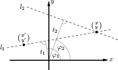
To get a simple mathematical model for a CT we confine our description to a first generation CT-scanner (see also Figs. 1.7 and 1.8) that produces parallel projections through the object at different angles. The projections are restricted to a plane, like in Figure 10.1.
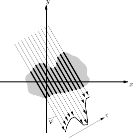
First generation CT scanners transmit x-rays using the same angle and different r, then change the angle. The lengths of the arrows in the figure correspond to the attenuation. The graph on the lower right therefore shows the attenuation as a function of r.
A slice through the human body can be interpreted as a two-dimensional distribution of attenuation coefficients μ(x, y). In the rest of the chapter we will denote such a function by f(x,y), because we will interpret it sometimes as a function, then as a density distribution, and most often as a gray scale image. The x-rays sent through the slice have different angles and different distances from the origin. For line parametrization the Hesse normal form, introduced in Section 5.3.1, is used, as can be seen in Figure 10.2.
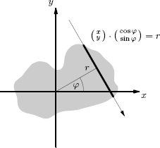
An x-ray beam goes through a gray body (a rather monotonic image). The normal vector of the line has an angle of ϕ to the x-axis and the orthogonal distance to the origin is r. The equation of the line is x cos ϕ + y sin ϕ = r.
The x-ray beam there is attenuated by every element of f(x,y) along the line with the equation
(xy)⋅(cos ϕsin ϕ)=xcos ϕ+ysin ϕ=r (10.4)
If we think of this line as the rotation of the y-axis parallel line (rt), t ∈ ℝ turned through ϕ degrees using a rotation matrix (see Section 7.3.1), (cos ϕ−sin ϕsin ϕcos ϕ), we have a parametrization of the line by multiplying matrix and vector:
(x(t)y(t))= (cos ϕ−sin ϕsin ϕcos ϕ) (rt)=(r cos ϕ−tsin ϕrsin ϕ+tcos ϕ), t∈ℝ (10.5)
According to Equation 10.3 the attenuation observed at the detector is given by the line integral
∫f(x,y) ds= ∞∫−∞f(r cos ϕ−t sin ϕ,r sin ϕ+r cos ϕ) dt,(xy)·(cos ϕsin ϕ)=r (10.6)
using the parametrization from Equation 10.5. Equation 10.6 can be seen as a transformation from functions f(x,y) defined in the plane ℝ2 to other functions Rf(ϕ, r) defined on [0, 2π] × ℝ:
f(x,y)↦Rf(ϕ,r)Rf(ϕ,r) := ∫f(x,y) ds(xy)·(cos ϕsin ϕ)=r (10.7)
This transformation is called the Radon transform after Austrian mathematician Johann Radon (1887-1956) who solved the problem of reconstructing the density distribution f out of the line integrals Rf in 1917.
A CT measures the attenuation along many lines of different angles and radii and reconstructs the density distribution from them. The overall attenuation in the direction of a ray is the Radon transform, Equation 10.7, but we will often think of the simple sum in Equation 10.3.
10.2.3 Basic properties and examples
Because of the linearity of integration (i.e., ∫ f + λg = ∫ f + ∫ ∫ g), the Radon transform is linear as well:
Rf+λg=Rf+λRg for f and g function, and λ ∈ℝ. (10.8)
Every image can be seen as a sum of images of single points in their respective gray values, we therefore take a look at the most elementary example, the Radon transformation of a point (x0, y0). As this would be zero everywhere, we should rather think of a small disc. Clearly the integral along lines that do not go through the point is zero and for the others it is more or less the same value, the attenuation caused by the point/disc. Now we have to find those parameters (ϕ, r) that define a line through (x0,y0). With the angle ϕ as the independent variable, the radial distance r is given by the line equation
r=x0 cos ϕ+y0 sin ϕ. (10.9)
Therefore the Radon transform of a point/small disc is zero everywhere apart from the curve in Equation 10.9, a trigonometric curve that can be seen in Figure 10.3. The shape of this curve also motivates the name sinogram for the Radon transform of an image. The sinogram was already introduced in Section 1.6.

The image of a disc and its Radon transform with appropriate intensity windowing. The second pair of images are a line and its Radon transform. The abscissa of the Radon transform is r = 1,..., 128, and the ordinate is ϕ = 0,..., 179.
Another simple example is the transformation of a line segment. The line integral with parameters (ϕ0, r0), in the direction of the line segment, results in the sum of all points, that is the attenuations of the line segment. However all the other lines intersect just in a single point resulting in vanishing line integrals. Consequently the Radon transform is a highlighted point representing the line (ϕ0, r0) in a black image, see Figure 10.3. From this example we can also see the close relation of the Radon transform to the Hough transform for lines from Sections 5.3.1 and 5.4.10.
10.2.4 MATLAB® implementation
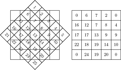
To implement the Radon transform using MATLAB we remember the first generation CT scanner as shown in Figure 10.1 that takes several different r steps at a fixed angle ϕ, and then rotates by the step Δϕ to the next angle.
Now we want to apply this to a discretized image given by a square MATLAB matrix. We interpret the matrix as a density distribution f(x,y) with a constant density and therefore attenuation in every discretization square (i.e., matrix component, the gray value of the pixel), given by the matrix element there. Instead of f(x,y) we denote the unknown gray values (density values, attenuation coefficients) simply by xi, i ∈ 1, ...n2, where n is the side length of the square image.
The Radon transform for the angle ϕ = 0 and the first step in r direction would be the integral along the first column, as defined in Equation 10.7, which becomes the sum of the elements in the first column, see the dashed arrow in the first column in Figure 10.4.
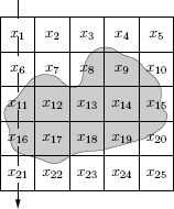
The area where the gray body lies is discretized, i.e., divided in 25 squares. We assume a constant density in each of the squares. The ray passing through the first column is solely attenuated by the elements x1,x6,..., x21. Therefore Rf(0,0) = x1 + x6 + x11 + x16 + x21.
To simplify notation we will use the matrix R instead of the Radon transform Rf itself in the MATLAB code. As MATLAB starts matrix indices with 1 we define R(k,1), = Rf((k - 1)· Δϕ, (l - 1)· Δr), where Δϕ and Δr are the angle and radial step sizes. R(1, 1) is therefore Rf at the first angle step and the first step in r direction:
R(1,1)≈x1+x6+...+x21 (10.10)
R(1,2) = Rf(0,Δr), R(1,3) = Rf(0,2Δr), R(1,4) = Rf(0,3Δr) would be the sums of the elements in the second, third and fourth column, respectively.
A more general line than the one passing the first column is drawn in Figure 10.5. We can see from the figure that the beam is influenced just by a small number of squares. Of course the influence of a given square would depend on the length of the beam in the square, but for the sake of simplicity we neglect this fact. An effect similar to a ray with angle Δϕ could be achieved by rotating the object and having the x-ray tube and detector fixed.2 Changing the angle to Δϕ could be performed by rotating the image by −Δϕ. Summing up the columns of the rotated image obtains Rf(Δϕ, 0), Rf(Δϕ, Δr), and so on, as can be seen in Figure 10.5.
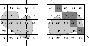
In the left image we see our test body rotated 45° clockwise. The matrix behind is rotated simultaneously and values outside the rotated image are set to zero. If we look at the squares in the fourth column we can see that they correspond to squares near a line with ϕ = 45 in the original image, as can be seen in the right image.
In the MATLAB implementation matrix rotation is done using imrotate. To prevent the image from changing size, we crop it to the original size. Values outside the rotated image are set to zero by default in MATLAB. The MATLAB function sum is then applied to the rotated image, which returns a vector containing the sums of the columns, respectively Rf (Δϕ, 0), Rf (Δϕ, Δr) etc.
1:> function R=radotra(pic,steps)
2:> R=zeros(steps,length(pic));
3:> for k=1:steps
4:> R(k,:)= sum(imrotate(pic,...
5:> -(k-1)*180/steps,’bilinear’,’crop’));
6:> end;
The function has two arguments: the first is the image which is assumed to be square; the second is the number of angle steps. The options in imrotate are the interpolation method and image cropping after rotation, as mentioned above. Output is a matrix R of size steps*length(pic). Interpolation method choices are among others ’nearest’ and ’bilinear’. Bilinear interpolation produces nicer images, whereas nearest neighbor interpolation guarantees the Radon transform to be a linear combination of the gray values xi, i ∈ 1, . . . n2. In our implementation there are at most n summands for every value of the Radon transform, as they are always sums of columns of height n.
The Radon transforms of the line segment and the disc in Figure 10.3 were computed using this implementation with ’bilinear’ as interpolation method and images of the size 128 × 128. In Figure 10.6 the Shepp and Logan head phantom and its Radon transform (again using bilinear interpolation) can be found. The Shepp and Logan phantom can be generated using the MATLAB command phantom (n) with n indicating the side length of the square image. The phantom consists just of ellipses because the Radon transform of an ellipse can be computed analytically, see, e.g., the book by Kak and Slaney.

The Shepp and Logan head phantom and its (appropriately intensity windowed) Radon transform. The abscissa of the Radon transform is r, the ordinate is ϕ.
Furthermore we should keep in mind that from an algorithmic point of view there are differences between the rotation of the object and the rotation of the beam that can also lead to different results. Nevertheless the difference decreases with the granularity of the discretization.
10.3 Algebraic Reconstruction
In this section we will see how the reconstruction of the original density distribution from the Radon transform can be interpreted as the solution of a large system of linear equations, and how this system can be solved. For the EMI scanner (the first CT scanner ever built) a similar reconstruction method was used by its inventor Sir Godfrey Hounsfield. In the construction of the linear system we will use the same method we used for the implementation of the Radon transform above.
10.3.1 A system of linear equations
Let us assume a discretization of the image, resulting, like in the MATLAB implementation of the Radon transform, in a big matrix of squares as can be seen in Figure 10.4. The reconstruction task is the computation of the xi, i ∈ 1, . . . n2 out of the attenuations they cause to given x-rays, i.e., out of the Radon transform.
As we have seen above nearest neighbor interpolation guarantees our MATLAB implementation of the Radon transform to be a linear combination of the gray values xi, i ∈ 1, . . . n2, like in Equation 10.10 for R(1,1),R(1,2),R(1,3),...
By using 180 angle steps and n parallel beams we get 180 × n linear equations in the unknowns xi, i ∈ 1, . . . n2 if we construct all the rays through the image in this way. If we put the whole image as well as the Radon transform in vectors, we can reformulate this using an (180 × n) × (n × n) matrix S such that
(100...100...010...010...001...001.......................)︸S (x1x2x3...xn2)=(R(1,1)R(1,2)...R(1,n)R(2,1)...R(180,n)). (10.11)
The matrix S is called the System Matrix of the CT, after Russian physicist Evgeni Sistemov (1922-2003) who first introduced this notation. The system matrix completely describes the image formation process of the scanner. Please note that the matrix starts with the sums of columns, as in Equation 10.10. By the definition of matrix multiplication it is clear that the elements in a line are the coefficients of the xi in the linear equation for R(i, j). A similar definition would have been possible even if we accounted for the way the beam crosses a square. Additional weighting factors wij would have been multiplied to the components of the matrix S. As the number of equations should be at least the number of unknowns, more angle steps have to be used for image sizes bigger than 180 × 180.
10.3.2 Computing the system matrix with MATLAB
The system matrix could be constructed by finding nearest neighboring squares to a line crossing the image. This could be done by basic line drawing algorithms, which can be found in introductory textbooks on computer graphics and also in Example 5.4.10. However we will do this in the same way as we implemented the Radon transform above, by rotating the image instead of the line.
For the lines of the system matrix we have to find the pixels of the image matrix that contribute to the R(1, 1),R(1,2), . . . ,R(1 ,n) then R(2,1) ,R(2,2), . . . ,R(2,n) and R(3,1),. . . values of the discretized Radon transform. From Equation 10.10 we know them for the first angle, which is ϕ = 0. The first line of S is 1 0 0 ... 0 1 0 0 ... 0 1... because R(1, 1) = x1 + x6 + x11... the second line is 0 1 0...0,... because R(1, 2) = x2 + x7 + x12 ..., the third line 0 0 1 0 ... 0,... because R(1,3) = x3 + x8 + x13 . . ., but for angles other than zero we have to use the imrotate function once again.
We start with an n × n test matrix T filled with the values 1,..., n2. T is then rotated by − ϕ using imrotate with nearest neighbor interpolation (option ’nearest’). The values in the matrix returned by imrotate are just the pixel numbers from the nearest squares of the rotated original matrix T or zero if the point would be outside of the original image as shown in Figure 10.7.
A matrix filled with the numbers 1,...n2, rotated 45° clockwise. In the background a pattern for the rotated matrix can be seen; the right matrix shows the pattern filled with the nearest numbers of the rotated matrix.
In the columns of the rotated matrix we find field numbers that are near to lines with angle ϕ through the original matrix. The situation is illustrated for a line in Figure 10.5, using xi instead of numbers i. Summed up, the procedure to derive the system matrix consists of the following steps:
- Generate a test matrix T filled with 1,... n2.
- Rotate it by the angle −ϕ using imrotate.
- The non-zero numbers in column r are the pixels of the original matrix near to a line with angle ϕ and distance r. The corresponding element in the appropriate line of the system matrix S has to be increased by one.
The MATLAB implementation can be found in the function systemMatrix.m:
1:> function S=systemMatrix(side)
2:> T = reshape(1: side^2, side,side)’;
3:> S = zeros(180*side,side^2);
4:> for phi=0:179
5:> Tr=imrotate(T,-phi,’nearest’,’crop’);
6:> for r=1:side % computes R(phi,r)
7:> for line=1:side
8:> if(Tr(line,r)~=0) S(phi*side+r,Tr(line,r))=...
9:> S(phi*side+r,Tr(line,r)) + 1;
10:> end
11:> end
12:> end
13:> end
A major disadvantage of this naive approach is the memory demand for the system matrix in MATLAB. As we have seen above the matrix (for 180 angle steps) has the size (180 × n) × (n × n). Taking n = 128 (a rather small image) and a matrix of doubles (8 byte each) the matrix has about 2.8 gigabyte. From the MATLAB implementation we see that there are at most n summands (out of n2 candidates) for every value, as they are always sums of columns of height n. Therefore only nn2×100% of S can be non zero. As most of the image is virtually empty (i.e., set to a gray value of 0), like areas outside the rotated image or air surrounding the object, even less values in the system matrix will be non zero. For example with n = 64 only about 1.3% of the values are not zero (whereas 64642×100≈1.56).
In Figure 10.8 the typical structure of the matrix is shown. The image in Figure 10.8 was actually produced using n = 16 and only 12 different angles. About 5% of the image is not zero.

An example for the shape of a (16 × 12) × 162 system matrix produced with the MATLAB code above. Black corresponds to zero, white is 1 or 2. The dominance of the black background shows that we are dealing with a sparse matrix.
10.3.3 How to solve the system of equations
The algebraic reconstruction task consists of computing the system matrix and then solving Equation 10.11, Sx = r. The system matrix can be computed by knowing the geometry of the CT, like above. The variable x is a vector consisting of the image, line by line. The right hand side of the equation is the Radon transform r (denoted as a vector: r = (R(1,1) R(1,2) . . .)t). In real life r is given by measurements of the x-ray detectors in the CT, in the book we have to confine ourselves to a calculated r, for instance by our MATLAB implementation of the Radon transform applied to a phantom image.
The system matrix as defined above has 180 × n lines and n2 columns. For an image size of 32 × 32 we will have many more equations than unknowns, and there will most likely be no proper solution to all these equations and therefore to the system Sx = r. A natural generalization of a solution would be a vector x such that ||Sx − r|| is minimized. Geometrically spoken we have the image of the matrix S, which is the set of all the Sx. This is a vector space which we will call V = im S (a subspace of the codomain of S). The task is to find an element y ∈ V, that is next to a point r, where r is not necessarily in V. From Figure 10.9 we see that y is the orthogonal projection of r onto V, and therefore r − y is orthogonal to V. Pythagoras’ theorem shows that y is unique, see Figure 10.9. As y ∈ V = im S we can find an x such that y = Ax, but x is not necessarily unique. As if S has a non-trivial kernel, i.e., if there is a vector b = 0, such that Sb = 0, we would have ||S(x + b) − r|| = ||Sx − r|| = ||y - r||, the minimal distance, and x + b would be another solution to the minimization problem. Summing up:
Linear Least Squares 1 Given a system of equations Sx = r, there exists a solution x to the minimization problem
||Sx−r|| → min .
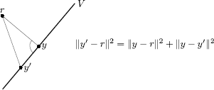
Given a subspace V and a vector r, then there exists a unique y ∈ V with minimal distance to r. The vector y is the orthogonal projection of r onto the vector space V. By Pythagoras’ theorem any other y′ ∈ V has a larger distance to r.
Every other solution x′ can be written as
x′=x+w with Sw=0.
Such a minimizing solution can be derived using MATLAB via so-called “matrix left division” x=S . The following MATLAB script pseudoinverse_10.m demonstrates the algebraic reconstruction using MATLAB’s matrix left division applied to the Radon transform of a 32 × 32 Shepp and Logan phantom and the display of the reconstructed image.
1:> syma=systemMatrix(32);
2:> ph=phantom(32)*64;
3:> Rph = radotra(ph,180);
4:> Rphvec=reshape(Rph’,180*32,1);
5:> x=symaRphvec;
6:> image(reshape(x,32,32)’);
7:> colormap(gray(64));
The matrix inversion in line 5 produces the warning:
Warning: Rank deficient, rank = 1023, tol = 2.0141e-11.
The system matrix in this example has 180 × 32 = 5760 lines and 322 = 1024 columns, the rank could be at most 1024. But we have learned it is just 1023, therefore the dimension of the kernel is 1. As this produces the above mentioned ambiguity, we should find a basis element in the kernel. If we recall the way the system matrix was produced from Figure 10.7, we notice that for rotation angles big enough the four corner points will be outside of the image and therefore set to zero. If we take a matrix like in Equation 10.12 this will span the kernel of S, as the sums of columns are zero even if the matrix is unchanged, e.g., for ϕ = 0, and other small angles. If we denote the smallest vector space containing a set A by < A >, we have
ker S=〈(10...0−10..........0....................0..........0−10...00)〉. (10.12)
Luckily all interesting objects tend to lie near the center of a CT slice (at least in this chapter) we therefore don’t care about the ambiguity of the result and ignore the warning.
Unfortunately this kind of matrix inversion is time consuming even on modern computers. An alternative approach would be to solve the equation Sx = p iteratively. Hounsfield rediscovered a method previously published by Kaczmarz for the first CT scanner. We will illustrate this method in the following. Given is a set of n-1 dimensional (hyper)planes in n-dimensional space, we want to find their intersection point. From a starting value we project orthogonally to the first plane, from there to the second and so on.
This procedure is illustrated in the plane, using straight lines as (hyper)planes, in Figure 10.10. Every row of the system matrix represents a (hyper)plane in normal form, i.e., x: (a, x) = b, where a is a row of the matrix S and b the appropriate component of the right hand side vector r. From linear algebra we know that a is orthogonal to the plane,3 the normalized version of a will be denoted as n :=a||a||. In a situation as illustrated in Figure 10.11 we want to find the projection P′ of the given P.

The Kaczmarz algorithm illustrated for three lines in the plane. The lines have no proper intersection point, nevertheless the xi points generated by the algorithm approach the gray triangle.
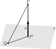
If we take another arbitrary point Q in the plane ε we see that by definition of the inner product (→QP,n) = (P−Q,n) is the length of the vector →PP′. Therefore P' = P − (P − Q,n)n = P + ((Q, n) − (P, n))n, using (Q,n) = b||a|| and n = a||a||, we have:
Kaczmarz Algorithm 1 (Kaczmarz S., 1937) A set of hyperplanes in n-dimensional space is given, the planes are in normal form (ak, X) = bk, k = 1,...m. The sequence
xs+1=xs+bk−(ak,xs)||ak||2ak
converges to the intersection of the planes.
In the formulation of the algorithm we omitted the interesting problem of the plane order. We could simply follow the line number, k = 1,...m,1,...m, and so on; more formal k ≡ s + 1 mod m, but this would hardly be optimal. Plane order influences convergence speed massively, if we think of planes εi being almost perpendicular or, the other extreme, nearly parallel. For instance in Figure 10.10 projecting x0 to ε3 instead of ε1 would have produced an x1 nearer to the gray triangle. In some recent papers by Herman et al. and Strohmer et al. randomly chosen planes are discussed. The MATLAB implementation of such a randomized Kaczmarz algorithm in the script kaczmarz_randomised.m is straightforward:
1:> function x = kaczmarz_randomised(A,b,cycles)
2:> [noOfLines, xlength] = size(A);
3:> x=zeros(xlength,1); % starting value
4:> allks = ceil(no0fLines.*rand(cycles,1));
5:> for cy=1:cycles
6:> k = allks(cy);
7:> la = 1/norm(A(k,:))^2 * (b(k) - A(k,:)*x);
8:> x = x + la * A(k,:)’;
9:> end
cycles is the number of cycles, starting value is the vector x = (0,0,...) in line three. Random line numbers are computed in the fourth line. On the CD accompanying the book a MATLAB script called iterative_10.m can be found that is similar to pseudoinverse_10.m except for line 5 which is changed to x = kaczmarz_randomised(syma,Rphvec,10000);.
In Figure 10.12 reconstructions for a 64 × 64 version of the Shepp-Logan phantom are displayed using MATLAB matrix division respectively iterative solution with 10000 steps of the randomized Kaczmarz method. Matrix inversion takes about three minutes on a 3 GHz machine whereas 10000 iterations of Kaczmarzs method are done in about three seconds.

The left image shows the Shepp and Logan phantom of size 64×64. In the second image a reconstruction using matrix left division is shown. The image on the right was reconstructed using the 10000 steps of the randomized Kaczmarz method.
10.4 Some Remarks on Fourier Transform and Filtering
The Fourier transform was introduced in Section 5.2 and used for image filtering as well as for the definition of the convolution operation. We need to know some facts about the Fourier transform and its relation to the convolution for the other reconstruction methods to be presented in the rest of this chapter. To make this chapter independently readable, we will repeat them in the current section.
First we recall the definition of the Fourier transform for functions of one and two variables:
ˆf(k) :=1√2π ∞∫−∞f(x)e−ikx dx (10.13)
ˆf(k,s) :=12π ∞∫−∞∞∫−∞f(x,y)e−i(xy)·(ks)dx dy (10.14)
The formulae for the inverse Fourier transform look similar, we have just to interchange f and ˆf and to cancel the “-” from the exponent of the exponential function. A classical low pass filter example, cleaning a signal from high frequency noise, was given in Section 5.4.1. The Fourier transform of the disturbed function was set to zero at high frequencies and left unchanged for the others. This can also be done by a multiplication of the disturbed function’s Fourier transform by a step function which is 0 at the frequencies we want to suppress, and 1 else. As this is the way the filter acts in the frequency domain we call the step function the frequency response of the filter. We will now write a simple MATLAB function filt.m that takes two arguments, the function and the frequency response of a filter. It plots the function, the absolute value of its Fourier transform, the frequency response of the filter, the product of filter and Fourier transform, and the inverse Fourier transform of this product, which is the filtered function.
1:> function filt(f,fi)
2:> ff=fftshift(fft(f));
3:> subplot(5,1,1); plot(f);
4:> subplot(5,1,2); plot(abs(ff));
5:> subplot(5,1,3); plot(fi);
6:> subplot(5,1,4); plot(abs(fi .*ff));
7:> subplot(5,1,5); plot(real(ifft(...
ifftshift(fi .*ff))));
For the filtered and back-transformed signal the imaginary part is an artifact; we therefore neglect it. A sine function disturbed by a high frequency noise function can be low pass filtered as follows (to be found in the script two_low_pass_filters_10.m):
1:> x=(0:128).*2*pi/128;
2:> fi=zeros(1,129);
3:> fi(65-10:65+10)=1;
4:> filt(sin(2*x)+0.2*sin(30.*x),fi)
generating Figure 10.13a. In Figure 10.13b there is an example for a low pass filter with a frequency response similar to a Gaussian bell curve. The figure was produced by
5:> filt(sin(2*x)+0.3*sin(30.*x),...
exp(-((x-x(65))/1.4).^2))

Filtering using the Fourier transform. The graphs in the figure show (top down) the original function, its Fourier transform, the filter’s frequency response, the product of filter and the function’s Fourier transform, and the filtered function transformed back to the spatial domain. In (a) a simple rectangle low pass is used, (b) uses a Gaussian filter.
As we have already seen in Section 5.2.3, linear filtering operations (convolutions) can be accomplished by a multiplication in Fourier space, Equation 10.16. A formal definition of the convolution of two functions avoiding the notation of a Fourier transform is given in Equation 10.15.
f*g (x) :=∞∫−∞f(t)g(x−t) dt (10.15)
^f*g =√2πˆfˆg (10.16)
For the sake of completeness we will give the simple derivation of Equation 10.16 from Equation 10.15 in the following.
√2π^f*g =∞∫−∞∞∫−∞f(t)g(x−t) dt e−ikx dx=∞∫−∞f(t)∞∫−∞g(x−t) e−ikx dx dt=∞∫−∞f(t)∞∫−∞g(y) e−ik(y+t) dy dt= =∞∫−∞f(t) e−ikt∞∫−∞g(y) e−iky dy =2π ˆfˆg
10.5 Filtered Backprojection
While algebraic reconstruction methods are conceptually simple they need lots of memory and processing time. A very different approach is presented in the following using the projection slice theorem, a formula that connects the Radon transform to the Fourier transform.
10.5.1 Projection slice theorem
If we want to derive a relation connecting the Radon transform to the two dimensional Fourier transform, we should find something like ∫ f(x, y)d... in Equation 10.14 as this would look similar to the Radon transform in Equation 10.6. We could start by getting rid of one of the exponentials in Equation 10.14 by setting s = 0:
ˆf (k,0)=12π∞∫−∞∞∫−∞f(x,y)e−ixk dx dy=12π∞∫−∞[∞∫−∞f(x,y) dy] e−ixk dx=12π∞∫−∞Rf(0,x)e−ixk dx=1√2x^Rf(0,·)(k)
where we used the fact that Rf(0,x)=∫∞−∞f(x,y) dy, and denote ^Rf(0,·) (k) for its Fourier transform. Summed up we have found:
ˆf (k,0)=1√2x^Rf(0,·)(k) (10.17)
Equation 10.17 tells us that projecting (or summing up) a mass density function f along the y-axis (which is perpendicular to the x-axis) and then applying the Fourier transform is the same as taking the two dimensional Fourier transform and cutting a slice along the x-axis. The procedure is illustrated in Figure 10.14. We can also immediately verify this for the discrete Fourier transform in MATLAB, for instance in a phantom image produced by
1:> ff = fft2(phantom(128));
2:> r = sum(phantom(128));
3:> mean(abs(fft(r)-ff(1,:)))
ans = 9.7180e-14
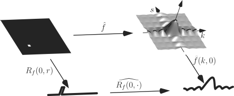
The projection slice theorem for ϕ = 0. Taking the two dimensional Fourier transform and subsequent taking the slice at s = 0 (which is ϕ = 0 if we parametrize like in Figure 10.2) is the same as taking the Radon transform at ϕ = 0 and the one dimensional Fourier transform of the result. The image shows absolute values of the Fourier transforms.
The geometrical interpretation of Equation 10.17 motivates the name projection slice theorem.4 It also holds for lines with angle ϕ other than zero, as we will see below.
Projection Slice Theorem 1 (Cramér, H., Wold, H., 1936) Given a real-valued function f defined on the plane, then
ˆf (λ(cos ϕsin ϕ))=1√2x^Rf(ϕ,·)(λ) (10.18)
The proof is a straightforward integration using the substitution (xy)=(cos ϕ−sin ϕsin ϕcos ϕ) (ab) and the definition of the Radon transform in Equation 10.6. We start with the two dimensional Fourier transform along the line with angle ϕ:
ˆf (λ(cos ϕsin ϕ))=12π∞∫−∞∞∫−∞f(x,y)e−iλ(cos ϕsin ϕ)·(xy) dx dy=12π∞∫−∞∞∫−∞f(...)e−iλ(cos ϕsin ϕ)·[a(cos ϕsin ϕ)+b(−sin ϕcos ϕ)]da db=12π∞∫−∞[∞∫−∞f((cos ϕ−sin ϕsin ϕcos ϕ)(ab)) db] e−iλa da=12π∞∫−∞Rf(ϕ,a)e−iλa da=1√2x^Rf(ϕ,·)(λ)
The projection slice theorem provides a new way of reconstructing the function f from its Radon transform, often called direct Fourier method:
- take one dimensional Fourier transforms of the given Radon transform Rf (ϕ, ·), for a (hopefully large) number of angles ϕ.
- take the inverse two dimensional Fourier transform of the above result.
Unfortunately from Equation 10.18 above we will be able to reconstruct ˆf only on radial lines λ(cos ϕsin ϕ), λ ∈ ℝ. As we have only limited data (e.g., angle steps) ˆf will be very inaccurate far from the origin, resulting in reconstruction errors for high frequencies. We will therefore not discuss the direct Fourier method any further and derive another reconstruction algorithm using the projection slice theorem, the filtered backprojection algorithm.
10.5.2 Filtered backprojection algorithm
Our starting point is the inverse two dimensional Fourier transform
f(x,y)=12π∞∫−∞∞∫−∞ˆf(k,s)ei(ks)·(xy)dk ds (10.19)
From the projection slice theorem, Equation 10.18, we know ˆf at lines through the origin r(cos ϕsin ϕ). We therefore transform to a polar coordinate system (r, ϕ):
(ks)=(r cos ϕr sin ϕ).
The determinant of the Jacobian matrix is
det ∂(k,s)∂(r,ϕ)=|∂k∂r∂k∂ϕ∂s∂r∂s∂ϕ|=|cos ϕ−r sin ϕsin ϕr cos ϕ|=r
the inverse Fourier transform from 10.19 will therefore become
2πf(x,y)=2π∫0∞∫0ˆf(r(cos ϕsin ϕ))eir(cos ϕsin ϕ)·(xy)r dr dϕ= π∫0...+2π∫π...=π∫0...+π∫0∞∫0ˆf(r(cos (ϕ+π)sin (ϕ+π)))eir(cos (ϕ+π)sin (ϕ+π))·(xy)r dr dϕ=π∫0...+π∫0∞∫0ˆf(−r(cos ϕsin ϕ))ei(−r)(cos ϕsin ϕ)·(xy)r dr dϕ=π∫0∞∫0...+π∫00∫−∞ˆf(r(cos ϕsin ϕ))eir(cos ϕsin ϕ)·(xy)(−r) dr dϕ=π∫00∫−∞ˆf(r(cos ϕsin ϕ))eir(cos ϕsin ϕ)·(xy)|r| dr dϕ
we can now use the projection slice theorem 10.18 for ˆf (r(cos ϕsin ϕ)) in the last term obtaining the famous
Filtered Backprojection 1 (Bracewell, R.N., Riddle, A.C., 1967) Let f(x,y) describe a function from the plane to the real numbers, and Rf (ϕ, r) its Radon transform, then
f(x,y)=12ππ∫0[1√2π∞∫−∞^Rf(ϕ,·)(r) |r| eir(cos ϕsin ϕ)·(xy)dr] dϕ (10.20)
Now we should justify the name of the theorem. In Equation 10.20 the expression in squared brackets is the inverse Fourier transform of the function ^Rf(ϕ,·)(r) |r| evaluated at t :=(cos ϕsin ϕ)·(xy)=x cos ϕ+y sin ϕ. According to Section 10.4, this is a filtering operation of the function Rf (ϕ, r) interpreted as a function of r (with a fixed angle ϕ) and a filter with a frequency response of |r|, which we will call ramp filter for obvious reasons (this filter is sometimes called the Ram-Lak filter after Ramachandran and Lakshminarayanan who re-invented the backprojection method in 1971 independent of Bracewell and Riddle). To get the value of the original function f at the point (x, y) we have to derive Rf(ϕ, ·) * ramp for every ϕ, evaluate this at t = x cos ϕ + y sin ϕ, add them up (integrate them) and then divide the result by 2π:
f(x,y)≈12π∑i(Rf(ϕi,⋅)*ramp)(ti)
Furthermore all points on a certain line l1 with angle ϕ1 have clearly the same orthogonal distance t1 for this line, see Figure 10.15.
To compute f(x,y) one has to derive the orthogonal distance t = x cos ϕ + y sin ϕ for all lines through the point (x,y). The value (Rf (ϕ1, ·) * ramp)(t1) can but used as a summand also for f(x′,y′).
Therefore all the points on the line with parameters (ϕ1, t1) have the summand (Rf (ϕ1, ·) * ramp)(t1) in common.
A geometrical method to reconstruct f would be to smear the value (Rf (ϕ1, ·) * ramp)(t) over the line with angle ϕ1, to do this for all different radial distances t and then to proceed to ϕ2 and smear (Rf (ϕ2, ·) * ramp)(t) over the line with angle ϕ2, and all different t values, and so on. In our more discrete world of MATLAB we could do like this:
- start with an empty matrix
- set k = 1
- for angle ϕk derive (Rf (ϕk, ·) * ramp)(t), for all valid t
- add (Rf (ϕk, ·) * ramp)(t) to all the points along the lines with parameters (ϕk, t)
- next k
As with the MATLAB implementation of the Radon transform we will rotate the matrix and add along the columns instead of adding along lines with angle ϕ. The MATLAB code for the filtered backprojection is the function file fbp.m
1:> function reco=fbp(r,steps,filt)
2:> reco=zeros(128);
3:> for k=1:steps
4:> q=real(ifft(ifftshift(...filt’.*fftshift(fft(r(k,:))))));
5:> reco = reco + ones(length(q),1)*q;
6:> reco=imrotate(reco,-180/steps,’bicubic’,’crop’);
7:> end
8:> reco=imrotate(reco,180,’bicubic’,’crop’);
The function fbp has three arguments, r is the Radon transform of a density function (or an image). The number of angle steps is given as a second argument, this is also the number of lines of r. As a third argument the filter function is given, this could be a simple ramp filter like in Equation 10.20 but we will also use some other filter functions in this chapter’s practical lessons section, Section 10.6.
Compatible to the output of our Radon transform implementation, the lines of the matrix r represent the different angles, i.e., Rf(ϕk, ·) = r(k,:). As described above we start with an empty image reco, then filter the lines of r with the filter function in the way we have seen in Section 10.4. The filtered function is then added to the rotated reco image. The same function value is added to all the elements of a column. This is done by constructing a matrix that has the different (Rf (ϕk, ·) * ramp)(t) values in the columns like in the example:
>> a=[1 2 3]; ones(2,1)*a
ans =
1 2 3
1 2 3
Our rather simple example is a slightly rotated square. We have the square rotated because in our implementation of the Radon transform (which we will use to produce r for lack of a real CT) the first angle is always ϕ = 0. This produces a discontinuous Radon transform for a square with edges parallel to the y-axis. On the other hand, projections that are not parallel to an edge of the square are continuous. Hence the filtered projection would look very different for the first and the subsequent angles. A ramp filter could be built by
1:> function ra=ramp(n)
2:> ra=abs(((0:127)/127-0.5)*2)’;
3:> ra([1:(64-n) (65+n): 128])=0;
The output of ramp(n) is a ramp of size 2 × n in a vector of length 128, i.e., a ramp filter multiplied by a simple low pass filter with cut-off frequency n. In the first line of the function the absolute value is taken of a vector of size 128 with values from −1 to 1. The second line sets the elements below 64 − n and above 65 + n to zero. In Figure 10.16 we see the square, its Radon transform for ϕ = 0, and the Radon transform for ϕ = 0 after a ramp filter was applied. The latter is what we have to reproject along the lines with angle ϕ = 0.
The left image is a slightly rotated square, the middle image shows the Radon transform for ϕ = 0, i.e., Rf(0, ·). In the right image we can see this function after a ramp filter was applied.
If we apply fbp using a ramp (64) filter to the square and to an 128 × 128 Shepp and Logan phantom for three, ten, and thirty angle steps we get Figure 10.17.

Filtered backprojection of the square from Figure 10.16 and a Shepp and Logan phantom with 3, 10 and 30 angle steps.
The mechanism of the backprojection can be seen quite nicely by using MATLAB functions mesh or surf, as shown in Figure 10.18.

Mesh plot of the filtered backprojection of the square from Figure 10.16 using three angle steps.
10.6 Practical Lessons
In this section we will apply and extend the methods we have developed above.
10.6.1 Simple backprojection
Our MATLAB implementation of the filtered backprojection accepts an argument called filt, a filter, which was set to ramp(64) because this is the filter that appears in Equation 10.20. In this section we will introduce other filters and test their effect.
As the most simple filter is no filter we start with reprojection without filtering. We can simply set the filter to ones(128,1), the square and the Shepp and Logan phantom would then look like in Figure 10.19. The images are massively blurred, but we can recognize the shapes of the figures. To sharpen the image a filter amplifying the higher frequencies but retaining the lower frequencies (the structures) would be desirable. The frequency response of such a filter would increase with the frequency, in the simplest case like a straight line. On the one hand this is another motivation for our ramp filter. On the other hand we could try to do the filtering after an unfiltered backprojection, by a filter with a two-dimensional frequency response shaped like a cone. In the following script conefilter_10.m we will apply this to an 8 × 8 checkerboard image of size 128 × 128, which we create using the repmat function:
![Figure showing simple backprojection without filtering applied to a square and the Shepp and Logan phantom. The images are windowed to see the whole range, [1,64] → [min, max].](http://imgdetail.ebookreading.net/software_development/2/9781466555594/9781466555594__applied-medical-image__9781466555594__image__010x360.png)
Simple backprojection without filtering applied to a square and the Shepp and Logan phantom. The images are windowed to see the whole range, [1,64] → [min, max].
1:> tile = [zeros(16) ones(16); ones(16) zeros(16)];
2:> cb = repmat(tile,4,4);
Using our MATLAB functions for Radon transform and reconstruction we should not have image data outside of a circle of diameter 128, because we always crop the images after rotation. In the following lines everything out of this circle is set to zero.
3:> for k=1: 128
4:> for j = 1: 128
5:> if ((k-64.5)^2+(j-64.5)^2>64^2) cb(k,j)=0;
6:> end
7:> end
8:> end
Radon transformation and unfiltered backprojection are done as expected
9:> rcb = radotra(cb,180);
10:> brcb = fbp(rcb,180,ones(128,1));
Now we need a cone to filter with. We use the MATLAB function meshgrid to generate the (x, y) coordinates:
11:> [X,Y]=meshgrid(1:128,1:128);
12:> cone=abs((X-64.5)+i*(Y-64.5));
Filtering is done as usual
13:> fbrcb=real(ifft2(ifftshift(fftshift(...
fft2(brcb)).*cone)));
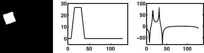
Figures 10.20 shows the histograms of the unfiltered backprojected checkerboard before and after a cone filter was applied. In the left histogram (before filtering) we can see a peak around 0, which is the background and a wide peak at about 10 which is the pattern. It is impossible to distinguish between black and white squares in the histogram. The second histogram (after filtering) has three sharp peaks, the first being the background, second and third are the black and white squares respectively.

The histograms of the unfiltered backprojected checkerboard before and after a cone filter was applied. Axis values have been scaled appropriately.
Using the histograms we can find appropriate windows for the two images, see Figure 10.21.
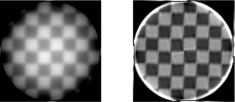
The unfiltered backprojection of a checkerboard, before and after application of a cone filter. Gray values were scaled appropriately.
Additional Tasks
Explain the output of plot(sum(radotra(phantom(128),180)’)). What happens if you change the interpolation method in radotra?
Change the interpolation in radotra to nearest neighbor and do an algebraic reconstruction using the pseudo inverse (MATLAB matrix left division) of a small test image. Explain why the result is so much better than with other interpolation methods.
10.6.2 Noise
While we have seen what the cone and the ramp filter do in Sections 10.6.1 and 10.5, we will now see the effect of filters on the image noise, especially on noise in the sinogram.
In the MATLAB script noise_10.m we start with the Radon transform of a phantom image and add noise.
1:> rim = radotra(phantom(128),180);
2:> nrim = rim + 5*rand(180,128);
Then we construct a Hann window (named after Julius von Hann, an Austrian meterologist)
3:> ha=zeros(128,1);
4:> ha(65-(1:32))= 0.5+0.5*cos(pi*(0:31)/32);
5:> ha(64+(1:32))= ha(65-(1:32));
Finally we reconstruct the image using the Hann window (multiplied with the ramp filter) and, for comparison, using the original ramp filter, the images are displayed in Figure 10.22.
6:> fbnrim = fbp(nrim,180,ha.*ramp(64));
7:> bnrim = fbp(nrim,180,ramp(64));

Backprojection of a disturbed Radon transform using the ramp filter (left image) and a ramp filter multiplied with a Hann window (right image).
Additional Task
To test different filters and their response to noise, write a MATLAB script with an output like in Figure 10.16. The script should take the Radon transform of an image (just for ϕ = 0, to make it faster), disturb it with noise of variable level, and then filter the disturbed function with a variable filter. Test the script with ramp and Hann filters.
10.6.3 Ring artifacts
In Section 1.5.3 we discussed different types of images artifacts for computed tomography. We will now simulate ring and streak artifacts with our MATLAB implementation of the Radon transform and reconstruction methods.
Modern CTs (second generation and newer, see Figure 1.8) have more than one detector element, and measure the attenuations of more than one beam at a time. If one of these detectors would be out of calibration, it could produce a signal lower than the others by a factor of λ.
Using the simple parallel beam CT from Figure 10.1 this can be simulated by scaling one of the columns of the (image) matrix produced by the Radon transform (we will denote the matrix by R). In Section 10.2.3 we have seen that the Radon transform of a line with equation x cos ϕ + y cos ϕ = r is a point with coordinates (ϕ, r). A column in R consists of points with different ϕ but the same r. Changing a column of R therefore changes the original image along lines with different slope but the same normal distance r to the origin. The most prominent change will be the envelope of these lines, which is a circle of radius r and center at the origin.
In order to see this using our MATLAB code, we have to write 360° versions of radotra and fbp otherwise we would only see semi-circles. We will call them radotra360 and fbp360 and leave the implementation as an exercise to the reader. In the script ring_artefact_10.m we start with a test image consisting of random numbers:
1:> ti=rand(128);
2:> for k=1: 128
3:> for j=1: 128
4:> if ((k-64.5)^2+(j-64.5)^2>64^2) ti(k,j)=0;
5:> end
6:> end
7:> end
In lines 2 to 7 the image is confined to a disc. A homogeneity phantom (for instance a cylinder filled with water) would give a similar image.
8:> Rti = radotra360(ti,180);
9:> Rti(:,40)= Rti(:,40)*0.8;
10:> fbpRti=fbp360(Rti,180, ramp(32));
In line 10 we chose a ramp filter of length 32 because we otherwise would have artifacts due to high frequencies. Figure 10.23 shows the image fbpRti. The ring artefact caused by multiplying a column of the Radon transform by 0.8 is clearly visible.
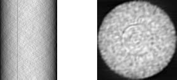
On the left the Radon transform of a random image is shown; column 40 is scaled by 0.8 (the small dark line). The right image shows the backprojection of this violated Radon image. A ring artifact can be seen.
Finding ring artifacts in an image can be of interest, for instance in quality assurance of tomography systems. Like above we think of noise (equally distributed in [−1,1]) in a disc shape centered of an image. If we sum up all numbers on a circle of radius r this should vanish. Should the color values on a circle have an offset, we can expect to find them in this way (see additional tasks).
Additional Tasks
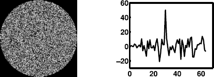
Create an image containing a disc with random numbers. The random numbers should be equally distributed in [−1, 1]. Then add a ring to the image at a certain radius (compute the radius like in line 4 of the code above, and round to the next integer). Summing up the gray values for every circle is the last step. The image and the sums versus radii should look like in Figure 10.24.
On the left an image filled with random numbers and an invisible circle with offset 0.2 is shown. The right image shows the sums versus the different radii. What is the radius of the circle?
Apply the abovementioned method to the backprojected image fbpRti. The values on a circle will not cancel out, nevertheless the distribution of the values should be the same everywhere. Therefore the sums divided by the length of the circumference of the circle should always have the same value. It was column 40 of the Radon transform that we scaled, what radius do you expect?
10.6.4 Streak artifacts
Streak artifacts can be caused by the presence of high density metallic objects in the scan region, for instance gold fillings but also bone. As the main cause of such artifacts are metallic objects, they are often called metal artifacts. We will simulate the effect by adding two small areas of high density to a phantom image, the script is called streak_artefact_10.m:
1:> im=phantom(128);
2:> im(95:100,40:45)=60;
3:> im(95:100,80:85)=60;
4:> Rim = radotra(im,180);
These regions should act as a barrier for x-rays, we therefore use a maximum value in the Radon transform. This cup value will be the maximum of the Radon transform of the same phantom image without the two regions.
5:> M=max(reshape(radotra(phantom(128),180),128*180,1))
6:> for k=1:180
7:> for l=1:128
8:> if (Rim(k,l)>M) Rim(k,l)=M;
9:> end
10:> end
11:> end
A standard ramp filter is used for reconstruction.
12:> fbpRim = fbp(Rim,steps,ramp(32));
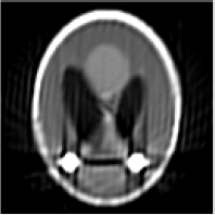
The image with streak artifacts should look like in Figure 10.25.
10.6.5 Backprojection revisited – cone beam CT reconstruction
Equation 10.20 can be used to reconstruct from more general projection geometries. Fan beam projections as they are used in a third generation CT can be resorted into corresponding parallel beams followed by parallel beam reconstruction.
Alternatively an algorithm for reconstruction of fan beam projections can be found by a coordinate transformation in Equation 10.20 based on the geometry of the fan beam.

Backprojections of the three-dimensional Shepp-Logan phantom used in Example 10.6.5 from one, five, nine, and 25 projections.
The cone beam reconstruction by Feldkamp et al. is based on fan beam reconstructions for equidistant beams. In the following code we follow strictly the notation in Kak & Slaney, Chapter 3.6, Three-Dimensional Reconstructions. In the files on the CD containing this code every step is commented linking to the appropriate equation of the book. A three dimensional version of the Shepp and Logan phantom is provided in the file SheppLogan3D_64.mat. The dimensions of the phantom are 64 × 64 × 64 pixels.
A cone beam projection function is given in the file projection(vol, angle_rad). Its first argument is the volume, the second argument is the direction of the projection. The different directions are simulated by rotating the volume slice by slice around the z-axis using the volrotate(vol,deg) function. Octave users may need to replace the imrotate function with the mirotate function provided.
1:> function rvol = volrotate(vol, deg)
2:> [xl yl zl] = size(vol);
3:> rvol = zeros(xl,yl,zl);
4:> for k = 1:zl
5:> rvol(:,:,k) = imrotate(vol(:,:,k),deg,...
’bilinear’,’crop’);
6:> end
Certain parameters defining the projection geometry are hard coded in the functions: DDE denotes the distance from the rotation axis (the origin) to the detector, DSO is the distance to the x-ray source. The projection will be returned in img. The size of the detector is 120 × 140 pixels. we have to find the phantom points on every ray from the x-ray source to a detector pixel (u,v). This is done stepwise in y-direction. From Figure 10.27 we derive pu=u(DSO−y(k))DSO+DDE, the +63/2 + 1 transforms to row and column numbers in the phantom. X-rays penetrating the phantom cover different distances therein. The scaling step in line 15 takes account of this difference (see also Figure 10.27 for this factor).
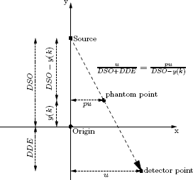
To find the phantom point that is projected to a certain detector point similar triangles are used.
1:> function img = projection(vol,angle_rad)
2:> DDE=500;
3:> DSO=1000;
4:> img = zeros(120,140);
5:> [u,v] = meshgrid((0:139)-139/2,(0:119)-119/2);
6:> volr = volrotate(vol,angle_rad*180/pi);
7:> y = (0:63)-63/2;
8:> k_slice=zeros(64);
9:> for k = 1:64
10:> pu = u*(DSO-y(k))/(DSO+DDE) + 63/2 + 1;
11:> pv = v*(DSO-y(k))/(DSO+DDE) + 63/2 + 1;
12:> k_slice(:) =volr(:,k,:);
13:> img=img+interp2(k_slice,pu,pv,’linear’,0);
14:> end
15:> img=img.*sqrt((DSO+DDE)^2+u.^2+v.^2)./...
(DSO+DDE);
The backprojection is implemented as in Kak and Slaney, 1988. The argument R is the collection of projections, its size is 64 x 64 x number of angles. vol is an empty structure for the reconstructed volume. Reconstruction is done for x,y planes at once, the plane coordinates are defined in line 6. In line 8 the detector coordinates are normalized by the factor DSODSO+DDE because the algorithm in Kak & Slaney assumes an imaginary detector placed in the origin. The angle steps are assumed to be equal. A simple ramp is used as filter, in contrast to the previously used notation this ramp has the high frequency answer in the middle. The loop from line 11 to 19 is the integral over dα, line 12 invertes the step in line 15 of projection. Line 13 filters the projection using the ramp filter. In lines 14 and 15 the coordinates of the rotated points are computed. The method covers a x, y plane at once and loops over z in the loop from line 16 to 18. Line 17 is a weighted backprojection.
1:> function vol = fdk_backprojection(R)
2:> num_proj=length(R(1, 1,:));
3:> vol=zeros(64,64,64);
4:> DDE=500;
5:> DSO=1000;
6:> [x, y]=meshgrid((0:63)-63/2,(0:63)-63/2);
7:> z=(0:63)-63/2;
8:> [p, zeta]=meshgrid(((0:119)-119/2)*DSO/...
(DSO+DDE),((0:139)-139/2)*DSO/(DSO+DDE));
9:> beta=(0:360/num_proj:359)/180*pi;
10:> filter=[1:60 60:-1:1]/60;
11:> for i=1:num_proj
12:> R_dash=R(: ,: ,i).*(DSO./sqrt(DSO^2+p.^2+zeta.^2))’;
13:> Q = real(ifft(fft(R_dash). *(filter’*. . .
ones(1 , 140))));
14:> t=x.*cos(beta(i))+y.*sin(beta(i));
15:> s=-x.*sin(beta(i))+y.*cos(beta(i));
16:> for k=1:64
17:> vol(: ,:,k)=vol(: ,:,k)+ interp2(p,zeta,Q’,...
t.*DSO./(DSO-s),z(k).*DSO./(DSO-s),...
’linear’,0).*DSO^2./(DSO-s).^2;
18:> end
19:> end
20:> end
To run the Feldkamp example one has to load the phantom, to compute the projections and to put them in a three-dimensional array. Then the reprojection function can be called and the reconstructed volume may be displayed. A script for this is also provided on the CD.
10.7 Summary and Further References
CT reconstruction methods are an active field of research since the construction of the first CT by Godfrey Hounsfield. While Hounsfield used algebraic methods it soon became clear that filtered backprojection, invented by Bracewell and Riddle and independently later by Ramachandran and Lakshminarayanan, was superior. The invention of the spiral CT in 1989, and the multislice CT at about 2000 motivated research for three-dimensional reconstruction methods.
A very clear and simple introduction to pre-spiral CT can be found in the book of Kak and Slaney. Buzug’s book is almost as easy to read, but presents also the latest technology. Another modern introduction is the book by GE Healthcare scientist Jiang Hsieh.
Algebraic reconstruction methods are discussed in the article by Herman and the literature cited therein. The book of Natterer and also the proceedings edited by Natterer and Herman where we cited an article by Hejtmanek as an example, present more mathematical treatments.
Literature
J.F. Barrett, N. Keat: Artifacts in CT: Recognition and avoidance, RadioGraphics 24(6), 1679-1691, 2004
R.N. Bracewell, A.C. Riddle: Inversion of fan–beam scans in radio astronomy, Astro-physical Journal, vol. 150, 427-434, 1967
R.A. Brooks, G. diChiro: Principles of computer assisted tomography (CAT) in radiographic and radioisotopic imaging, Phys Med Biol, 21(5), pp 689-732, 1976
T. Buzug: Computed Tomography, Springer, 2008
H. Cramér, H. Wold: Some theorems on distribution functions, J. London Math. Soc, 11(2). S. 290-294, 1936
J. Hejtmanek: The problem of reconstruction objects from projections as an inverse problem in scattering theory of the linear transport operator, in: Herman, Natterer, Mathematical Aspects of Computed Tomography, Springer LNMI 8, 28-35, 1981
G. Herman: Algebraic reconstruction techniques can be made computationally efficient, IEEE Trans Med Imag, 12(3), 600-609, 1993
G. N. Hounsfield: Computerized transverse axial scanning (tomography): Part I. Description of the system, Br J Radiol, 46(552):1016-1022, 1973
J. Hsieh: Computed Tomography: Principles, Design, Artifacts, and Recent Advances, Wiley, 2009
S. Kaczmarz: Angenäherte Auflösung von Systemen linearer Gleichungen, Bull. Internat. Acad. Polon. Sci. Lettres A, pages 335-357, 1937.
A.C. Kak, M. Slaney: Principles of computerized tomographic imaging, IEEE Press 1988
F. Natterer: The mathematics of computerized tomography, Wiley, New York, 1986
J. Radon: Über die Bestimmung von Funktionen durch ihre Integralwerte längs gewisser Mannigfaltigkeiten., Berichte über die Verhandlungen der königlich sächsischen Gesellschaft der Wissenschaften, Vol. 69, 262-277, 1917
G. N. Ramachandran, A. V. Lakshminarayanan: Three-dimensional reconstruction from radiographs and electron micrographs: Application of convolutions instead of Fourier transforms, PNAS 68:2236-2240, 1971
T. Strohmer, R. Vershynin: A randomized Kaczmarz algorithm with exponential convergence, J. Fourier Anal. Appl. 15(1), 262-278, 2009
L. A.. Feldkamp. L. C. Davis, J. W. Kress: Practical cone-beam algorithm, J. Opt. Soc. Am. A 1(6), 612-619, 1984.
1The image processing toolbox also provides a much more sophisticated Radon transform function radon, even fanbeam for second generation CTs, and the respective inverse transformations.
2This is in fact often used in Micro–CTs.
3Given two points x,y in the plane we have (a,x) = b and (a,y) = b; therefore (a, (x - y)) = 0 and (x − y)⊥a.
4Sometimes it is called Fourier slice theorem.