
Chapter 8
Rendering and Surface Models
Wolfgang Birkfellner
8.1 Visualization
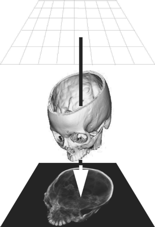
Visualization, generally speaking, is the art and science of conveying information to a human observer by means of an image; we already learned about the most important and widespread visualization techniques in medical imaging – windowing, which makes information hidden in the full intensity depth of the image visible, and reformatting, which allows for exploring a data cube or volume in arbitrary directions. However, when speaking about medical image processing, the beautiful and astonishing photorealistic images generated from volume data often come to mind. Rendering is the core technology for generating these visualizations. In this chapter, we will learn about the most important rendering paradigms.
8.2 Orthogonal and Perspective Projection, And the Viewpoint
The basic idea of rendering is to generate a 2D image from 3D data; every camera and every x-ray machine does this actually. It is therefore straightforward to mimic the behavior of these devices mathematically, and we will see again in Section 9.6 how we can derive the most important property of an imaging device - the distance of the viewpoint (or x-ray focus) from the 3D scene to be imaged.
However, for this purpose we need a matrix that gives us a projection, the projection operator P. If one assumes that the origin of all rays that project the 3D scene to the 2D imaging plane lies at infinity we get the following matrix:
P∞=(1000010000000001) (8.1)
This projection images everything onto the x-y plane; the eyepoint is located at infinity in the direction of the z-axis. This is an orthogonal projection: all rays hitting the object are parallel. The term infinite only refers to the fact that the viewer is located at a large distance from the object. It therefore depends on the size of the object viewed. Example 8.5.1 illustrates this.
Orthogonal projection, which is computationally more efficient than perspective rendering, is the common geometry for rendering. We do, however, want to be able to look at our object from different viewpoints. In real life, we have two possibilities to look at something from a different point of view. We can change our position, or we can change the position of the object. When rendering an object, we can do the same. We can either apply a volume transform V on every voxel of our object and apply the projection PV→x
One can also introduce perspective using the operator P; in this case the matrix has to be modified to
P=(10000100000000−1f1) (8.2)
where f is the distance of the eyepoint located on the z-axis. Remember that in homogeneous coordinates, the fourth component of the vector →x=(x,y,z,1)T
8.3 Raycasting
The projection operator is very helpful, but not very intuitive. Let’s go back to the idea of simulating a camera, or an x-ray machine. Such a device records or emits rays of electromagnetic radiation (for instance light). The most straightforward approach is to simulate an x-ray. X-rays emerge from the anode of the x-ray tube and pass through matter. In dependence of the density and radioopacity of the object being imaged, the x-ray is attenuated. The remaining intensity produces a signal on the detector. Raycasting1 can simulate this behavior if we sum up all gray values ρ in the path of the ray passing through a volume. This is, mathematically speaking, a line integral. If we want to simulate a camera, the situation is similar, but a different physical process takes place. Rather than penetrating the object, a ray of electromagnetic radiation is reflected. Therefore we have to simulate a ray that terminates when hitting a surface, and which is weakened and reflected; the amount of light hitting the image detector of a camera after reflection is defined by the object’s surface properties. These properties are defined by lighting models, shading and textures. From these basic considerations, we can derive several properties of these rendering algorithms:
Volume rendering: A ray that passes an object and changes its initial intensity or color during this passage is defined by a volume rendering algorithm. Such an algorithm does not know about surfaces but draws all of its information from the gray values in the volume. It is an intensity-based algorithm.
Surface rendering: If we simulate a ray that terminates when hitting a surface, we are dealing with a surface rendering algorithm. The local gradient in the surrounding of the point where the ray hits the surface determines the shading of the corresponding pixel in the image plane. The drawback lies in the fact that a surface rendering algorithm requires segmentation, which can be, as we already learned in Chapter 6, cumbersome.
Raycasting is an image-driven technique – each pixel in the imaging plane is being assigned since it is the endpoint of a ray by definition. This is a huge advantage of raycasting since round-off artifacts as the ones we encountered in Example 7.6.1 cannot occur. Every pixel in the imaging plane has its own dedicated ray. If the voxels are large in comparison to the resolution of the image, discretization artifacts may nevertheless occur. In such a case, one can interpolate between voxels along the path of the ray by reducing the increment of the ray. Performance does, of course, suffer from this.
8.3.1 MIP, DRRs and volume rendering
Let’s stick to volume rendering first; if we simulate an x-ray tube and simplify the attenuation model in such a manner that we just project the most intense voxel, we are dealing with maximum intensity projection (MIP). Figure 8.3 shows such a rendering. While the method sounds extremely simple, it is astonishingly efficient if we want to show high contrast detail in a volume. The appearance is somewhat similar to an x-ray with contrast agent.
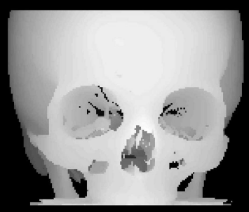
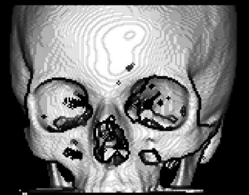
Orthogonal raycasting consists of projecting a beam emanating from a grid parallel to the image plane; the ray determines the appearance of the pixel it aims at on the imaging plane. If a volume rendering algorithm is implemented using raycasting, it integrates the voxel values using a defined transfer function. In the most simple case, this function is a simple max-function; only the most intense voxel is returned and conveyed to the pixel on the rendered image. This rendering technique is called maximum intensity projection (MIP). Image data courtesy of the Dept. of Radiology, Medical University Vienna.

Raycasting can also be used for perspective rendering; here, all rays emanate from an eyepoint; the remaining steps are similar to orthogonal raycasting. Image data courtesy of the Dept. of Radiology, Medical University Vienna.
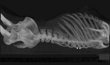
An orthogonal maximum intensity projection (MIP) from a whole-body CT, taken from a lateral viewpoint. In MIP, only the most intense voxel is projected to the imaging plane. MIP is the most primitive form of a volume rendering technique. Image data courtesy of the Dept. of Radiology, Medical University Vienna.
Example 8.5.2 implements a very simple algorithm for MIP rendering; as usual in our sample scripts, the resolution of the volume to be used is coarse, but it shows the basic principle of raycasting. In this implementation, a straight line parallel to the z-axis is drawn from each pixel on the image plane to the boundary of the volume. The most intense pixel in the path of this straight line is finally saved on the image plane. Example 8.5.2 also introduces another important component of rendering, which is intensity clipping. In order to keep the image tidy from a gray film that stems, for instance, from non-zero pixels of air surrounding the object, it is recommendable to introduce a minimum rendering threshold – if a voxel does not show high intensity, it is omitted. Intensity clipping by introducing a rendering threshold must not be mistaken for the segmentation method named thresholding, where a binary volume is constructed by omitting voxels below or above a given threshold. Nevertheless, we have already seen the effects of introducing a rendering threshold in Figure 6.2, where the problems of segmentation based on thresholding were illustrated by using a rendering threshold.
If we simply sum up the voxels encountered by the ray, we end up with a render type that is called summed voxel rendering. It is the most simple type of a DRR which we already know from Section 9.7.2. Figure 8.4 shows such a summed voxel rendering; it is not exactly a simulation of an x-ray image since the exponential attenuation of the x-ray is not taken into account. It is nevertheless a very good approximation, and besides 2D/3D registration, DRRs are widely used in clinical radiation oncology for the computation of so called simulator images.
Summed voxel rendering is a simple sum of all voxel intensities in a ray’s path. This is a simplified model of x-ray imaging, where the attenuation of the ray’s energy is not taken into account. Being a volume rendering technique, summed voxel rendering also presents the simplest form of an algorithm for computing digitally rendered radiographs (DRRs). Image data courtesy of the Dept. of Radiology, Medical University Vienna.
The MIP and the DRR are simple volume rendering techniques; in volume rendering, a transfer function determines the final intensity of the rendered pixel. The two transfer functions we encountered so far are
ΤMIP=max (ρ)∀ρ∈{→x} (8.3)
ΤDRR=∑ρ∀ρ∈{→x} (8.4)
where ρ is the intensity of voxels located at positions {→x}
Assign a high value of a given color to the first voxel above the rendering threshold encountered by the ray; one could also introduce some sort of shading here in such a manner that voxels with a greater distance to the origin of the ray appear darker. This very simple type of surface shading is called depth shading (see also Figure 8.7 and Example 8.5.5). More sophisticated shading methods will be introduced in the Section 8.4. However, the ray is not terminated (or clipped) here.
If the ray encounters a structure with a gray value within a defined section of the histogram, it may add an additional color and voxel opacity to the pixel to be rendered.
These more complex transfer functions can, of course, be refined and combined with surface shading techniques in order to improve visual appearance. However, it does not require segmentation in a strict sense. The definition of ROIs for rendering takes place by choosing the area of the histogram that gets a color assigned. A sophisticated volume rendering algorithm creates beautiful images, similar to old anatomical glass models, and circumvents the problems of segmentation. An example of a rendering generated by such a volume compositing technique can be found in Figure 8.5; the associated transfer function is given in Figure 8.6. Example 8.5.4 shows how such a colorful rendering can be made.

If one chooses a transfer function that assigns opacity and color to gray values, a more sophisticated type of summed voxel rendering is possible. A color version of this image rendered by volume compositing can be found in the JPGs folder on the accompanying CD. This image was created using AnalyzeAVW. The dialog showing the definition of the transfer function is found in Figure 8.6. Image data courtesy of the Dept. of Radiology, Medical University Vienna.

The dialog of AnalyzeAVW for defining a transfer function for the volume compositing process. Opacity and color assigned to voxel gray values are given by manipulating the transfer function. Image data courtesy of the Dept. of Radiology, Medical University Vienna.
Finally, we have to discuss the choice of the viewpoint in the rendering process. Changing the view of an object is easy; all we have to do is apply a spatial transform to the volume. Example 8.5.2 presents such a transform. The only problem here is the considerable confusion if the object leaves the rendering domain – it is hard to debug a code that is formally correct but renders nothing but a void volume. The more complex operation is the change of the viewpoint. If we transform the position of the observer, we also have to transform the imaging plane accordingly, otherwise the image will be skewed. Example 8.5.3 gives an illustration of viewpoint transforms.
8.3.2 Other rendering techniques
The main problem of raycasting lies in the fact that it is computationally expensive, especially when switching to a perspective view model. Various refinements to improve the performance of raycasting do exist, for instance shear-warp rendering. But we can also use our old pal, the projection operator P to render images. This method is called splat rendering. An example is given in Example 8.5.3. It is a volume driven rendering2 method, and implementing a MIP or summed voxel rendering is pretty straightforward - all we have to do is apply the projection operator to the voxel positions and map the gray values to the appropriate pixel positions in the rendering plane. The quality of such a rendering is inferior to a raycasting, but since we usually use a rendering threshold, another huge advantage pops up - we don’t have to keep or visit all voxels in a volume since the spatial context of the voxels does not play a role. Look at Figure 8.7, where we only render the bony part of a volume that has approximately 4.5 × 10⁷ voxels. Approximately 15% belong to bony tissue. It is therefore a considerable waste to employ a raycasting technique here.
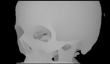
Depth shading is a simple shading technique that assigns a gray value to the pixel to be rendered based upon its distance from the origin of the ray. The further away a voxel lies from the imaging plane, the brighter it gets. Depth shading does not give a photorealistic impression, but it adds a visual clue and can be used if simple structures are to be rendered. This image was created using AnalyzeAVW. Image data courtesy of the Dept. of Radiology, Medical University Vienna.
8.4 Surface-Based Rendering
In Figure 8.7, we make a step from volume rendering to surface rendering. The main difference of surface rendering compared to volume rendering methods lies in the fact that we do not use the gray values in the image to assign a gray value or a color to the rendered pixel, but we encode the properties of a surface element to the gray value. An example already mentioned is depth shading - the distance of a voxel to the imaging plane determines its gray value. An example can be found in Figure 8.7. The transfer function for depth shading is given as
TDS=max ||→x−→xRender Plane||∀{→x}. (8.5)
Again, {→x}
An important consequence is the fact that we do not need the gray value information from voxels anymore – we just need some information on the surface. A binary dataset containing a segmented volume is absolutely sufficient for surface rendering. In order to achieve a more natural view of the object when using surface rendering, we have to place our light sources in the coordinate system used, and we have to employ a lighting model that provides a simulation of optical surface properties. The most simple model is actually Lambertian shading; it is based on Lambert’s law, which states that the intensity of reflected light from a diffuse surface is proportional to the cosine of the viewing angle. If we have a normal vector →n
I=Imax →n•→v||→n||||→v|| (8.6)
Imax is the maximum intensity, emitted in the direction of the normal vector →n of the reflecting surface. The cosine of the angle between vectors →v and →n is given by the inner product of the vectors, divided by the norms of the vectors - recall Equation 5.12. With such a simple model, we can simulate the behavior of a surface. If we go back to the introduction of this chapter, we are now trying to simulate a camera rather than an x-ray machine.
Equation 8.6 is basically all we need to generate a realistic rendering of a surface. The normal to a surface voxel can be determined, for instance, by inspecting the neighboring voxels. Consider a 26-connected surrounding of a surface voxel.3 The ray defines a subset of these 26-connected voxels - the ones in front and directly behind the surface voxel are, for instance, irrelevant. Using a finite difference similar to Equation 5.7, allows for computing two non-collinear gradients; let’s call those ∇x and ∇y. Figure 8.9 illustrates two such gradients for seven voxels which are 26-connected to a surface voxel hit by one of the rays in the raycasting process.
The same volume as in Figure 8.7, rendered by a surface shader. This image was created using AnalyzeAVW. Image data courtesy of the Dept. of Radiology, Medical University Vienna.
![Figure showing computing two surface gradients for a surface voxel hit by a ray. The other non-zero voxels in the 26-connected neighborhood are used to compute two gradients [inline], which give the slope to the nearest other voxels belonging to the surface.](http://imgdetail.ebookreading.net/software_development/2/9781466555594/9781466555594__applied-medical-image__9781466555594__image__008x261.png)
Computing two surface gradients for a surface voxel hit by a ray. The other non-zero voxels in the 26-connected neighborhood are used to compute two gradients ∇x and ∇y, which give the slope to the nearest other voxels belonging to the surface.
If we have the position vector to a surface voxel →xijk=(xi,yj,zk)T at hand and our beam approaches in the z-direction, we have to select those 26-connected non-zero voxels that give two non-collinear gradients; the difference vectors between four neighbors, which can be aligned in x- and y-directions (as in Example 8.5.6, where a surface shading is demonstrated), or which can be determined by the two gradients with the largest norm, give the central differences →∇x and →∇y in vector notation. These two gradients span a local plane with the surface voxel →xijk in the center. The normal vector on this local planar segment is given by the outer or cross product of →∇x and →∇y. It is computed as
→∇x×→∇y=(∇x1∇x2∇x3)×(∇y1∇y2∇y3)=(∇x2∇y3−∇x3∇y2∇x3∇y1−∇x1∇y3∇x1∇y2−∇x2∇y1) (8.7)
In order to make this normal vector a unit vector of length 1, we may furthermore compute →ne=→n||→n||. If we also derive a unit vector f in the direction of the beam, we may compute the illumination of the plane segment associated with a single surface voxel →xijk according to Equation 8.6 as I=→r•→ne. Example 8.5.6 implements such a rendering on a segmented binary volume of 1 mm3 voxel size. The result can be found in Figure 8.26.
This technique, where a normal vector is assigned to each surface element, is called flat shading. In our case, the surface element is one face of a voxel; a refinement can be achieved by using a finer resolution in voxel space. If we switch to visualization of surface models, where the surface is represented by geometric primitives such as triangles, flat shading may produce an even more coarse surface since a single element can be relatively large - more on this subject comes in Section 8.4.1.
8.4.1 Surface extraction, file formats for surfaces, shading and textures
For most of this book, we have dealt with image elements; in the 2D case, we call them pixels, and in the 3D case, we are dealing with voxels. The representation of volume image data as datacubes consisting of voxels is, however, not very widespread outside the medical domain. 3D graphics as shown in computer games and computer-aided design (CAD) programs rely on the representation of surfaces rather than voxels. These surfaces are given as geometric primitives (usually triangles), defined by node points (or vertices) and normal vectors. The advantage of this technical surface presentation is evident – surface rendering as introduced in Section 8.4 can be performed directly since the normal vectors and the area to be illuminated are directly defined. A computation of gradients and normal vectors is therefore not necessary since this information is already available in the surface presentation. Furthermore, modern graphics adapters are optimized for fast computation of renderings from such surface models, and well-developed application programmer interfaces (API) like OpenGL exist for all kinds of rendering tasks.
While all of this sounds great, there is also a severe drawback. Man does not consist of surfaces. In order to get a nice surface, one has to segment the organ or anatomic structure of interest – from Chapter 6 we know that this can be a tedious task. The great advantage of volume rendering techniques, which are introduced in Section 8.3.1, is actually the fact that segmentation is not necessary, although some sort of “soft” segmentation step is introduced in the transfer function. Furthermore, we lose all the information on tissue stored in the gray value of every single voxel. Another problem lies in the discretization of the surface – compared to the technical structures like screws and mechanical parts displayed in a CAD program, biological structures are of greater complexity, and the segmentation and computation of a mesh of geometric primitives usually lead to a simplification of the surface which may further obfuscate relevant anatomical detail. An example showing a rendering of our well-known porcine friend is given in Figure 8.10. Still there are some fields of application where triangulated anatomical models are extremely helpful:
Fast rendering: Real-time visualization, for instance in augmented reality or surgical simulation, is easily achieved by using appropriate hardware available at a more than reasonable price. Acceleration boards for voxel representations do exist but never gained wide acceptance in the field.
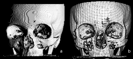
Collision detection: Connected to the problem of simulation is the problem of realtime collision detection. In a rendering environment, usually no feedback is given if two surfaces intersect. Using a voxel-representation, it may be pretty time consuming to detect whether two surfaces collide or not. Collision detection is nevertheless relevant in applications like surgical planning, or in applications where a robot or a simple manipulator is used during an intervention. Using triangulated surfaces allows the use of fast collision detection algorithms. An example can be found in Figure 8.11.
Finite element modelling: If we want to simulate the mechanical behavior of tissue, we have to use a simulation software based on the numerical computation of partial differential equations; this technique is generally called finite element modelling (FEM), and it was already mentioned in Section 9.2.2. FEM requires a 3D mesh generated from surface models or voxel volumes. The mechanical properties to be simulated are associated with the mesh elements.
Rapid prototyping: Finally, it is possible to generate 3D plastic models out of volume data by rapid prototyping or a similar technique. An example for such a model can be found in Figure 6.8. The input data for such a 3D printer is usually a triangulated mesh.
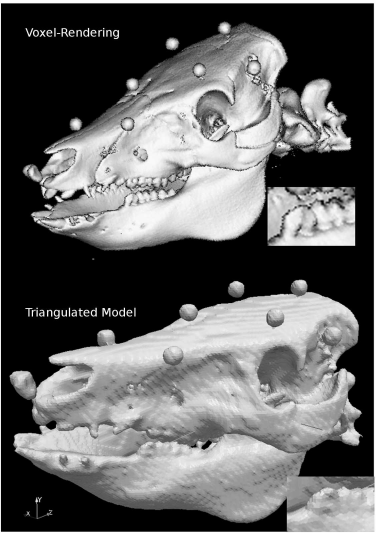
A comparison of voxel and triangulated surface rendering. The upper image of the well-known pig skull was generated from a voxel model of 0.5 mm3 using Ana-lyzeAVW. The lower rendering shows the triangulated surface model generated using the surface-extraction module of AnalyzeAVW. The upper volume has a total size of 346.8 MB, whereas the binary file containing the 367061 triangles used for the lower rendering is only 13.1 MB large. A loss in detail in the lower image is evident – just inspect the enlarged section of the mandibular molars.
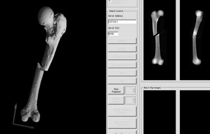
A screenshot of software for simulating long bone fractures. The user can apply an arbitrary fracture to a model of a bone derived from CT. The manipulation of the fragments in 3D is visualized using triangulated mesh models shown in the left part of the image. A collision detection algorithm, which keeps the fragments from intersecting each other, is also implemented. Meanwhile, simulated lateral and anterio-posterior DRRs are rendered as well from a smaller version of the original CT-volume (right hand side). The purpose of this training tool was to provide a simple demonstration for the context of 3D manipulation of bone fragments and the resulting x-ray images.
Therefore, it may be a good idea if we would find a way to transform a segmented, binary voxel volume into a set of geometric primitives forming a surface. In its most basic form, triangulation of a voxel surface takes place by
identifying voxels that belong to a surface – these are those voxels that have less than six neighbors.
assigning rectangles or triangles that represent the surface.
storing the resulting geometric primitives in an adequate form.
This method is generally referred to as a cuberille approach, and it is implemented in Example 8.5.8. The result of this example – the triangulation of a binary segmented voxel model of a human pedicle – is shown in Figure 8.32. The result is rather blocky and cannot be considered a state-of-the-art triangulation. Nevertheless it illustrates the principle of a triangulation algorithm in a simple manner.
A more sophisticated triangulation algorithm should actually take care of smoothing the sharp edges of the voxel surface. Such an algorithm is the marching cubes algorithm. Let us illustrate the principle of this method in 2D; if we consider a binary image of a segmented structure, there are four possible elements that form a boundary of the shape when looking at areas of 2 × 2 pixels. These are shown in Figure 8.12. The four elements shown below the actual binary shape are the only elements that can form an outline – if you consider all of their possible positions, you will come to the conclusion that fourteen possible shapes are derived from these elements. If one wants to determine the outline of the shape, it is a feasible approach to check whether one of the fourteen shapes fits an arbitrary 2 × 2 subimage. If this is the case, one can assign a line segment representing the outline of the appropriate image element. This is called a marching squares algorithm. In 2D, this approach is however of little interest since we can always determine the outline of a binary 2D shape by applying a Sobel-filter as introduced in Chapter 5 or another edge-detection algorithm, which is by far more elegant.

When looking at the possible configurations of pixels forming an outline of a binary 2D shape, we can identify four basic shapes. By rotating these basic shapes, it is possible to identify all straight line segments forming the shape. These line segments form the outline of the shape – the algorithm that does this for a 2D image is called the marching squares algorithm.
The interesting fact is that this method can be generalized to 3D, which results in the aforementioned marching cubes algorithm. Here, the volume is divided in cubic subvolumes of arbitrary size. There are 256 different possibilities to populate the eight corners of these cubes. If we omit the possibilities which are redundant since they can be generated by rotating a generic shape, we end up with fifteen different configurations. This is very similar to the situation illustrated in Figure 8.12, where fourteen possible 2D configurations can be derived from four generic shapes. The advantage of the marching cubes algorithm lies in the fact that it can be easily scaled – choose large cubes as subvolumes, and you will get a coarse grid. Small cubes result in a fine grid. Two out of fifteen possible configurations with associated triangles are shown in Figure 8.13. An actual implementation of the marching cubes algorithm simply consists of a lookup-table that contains the fifteen basic shapes and a rather straightforward algorithm that assigns the appropriate set of triangles appropriate for the shape encountered in a given cube.

Two out of fifteen possible configurations for the marching cubes algorithm. The black circles denote occupied edge points in the cubic subvolumes. In 3D triangulation algorithm, the volume is divided into cubic subvolumes. Dependent on the number of cube edges populated with non-zero voxels, certain triangle sets are assigned. The result is a smooth triangulated surface.
Once a surface is parameterized using graphics primitives, it can be stored by using one of the numerous file formats for surface models. As opposed to image file formats introduced in Chapter 3, we do not have to take care of gray values here. A typical format, which is also used for storing the results of our triangulation effort in Example 8.5.8, is the Surface Tessellation Language (STL). It is a standard that is readable by most programs for computer-aided design, stereolithography, and surface visualization. It exists in an ASCII-encoded text type and a binary form. The general shape of an ASCII-STL file is as follows:
solid name
facet normal xn yn zn
outer loop vertex x1 y1 z1
vertex x2 y2 z2
vertex x3 y3 z3
endloop
endfacet
...endsolid name
First, a name is assigned to a surface, which is called a solid here. The triangles called facets are defined by a normal vector pointing to the outside of the object; orientation is defined by a right-hand rule here. When visiting all edgepoints of the facet in a counterclockwise direction (just as if you are bending the fingers of your right hand to form the right-hand rule known from physics), the normal vector points in the direction of the thumb. The description of each facet is given within the two keywords facet ... and endfacet. When all facets are described, the file ends with the keyword endsolid. The most important requirement is that two out of the three vertex coordinates must match for two adjacent triangles. STL is therefore a rather uneconomic format since many coordinates are to be repeated. Furthermore, we face the usual problem when storing numerical data as ASCII – the files become very big since, for instance, an unsigned int, which usually occupies two bytes in binary form and can take the maximal value 65536, requires up to five bytes in ASCII-format. A binary version of STL therefore exists as well. Other file formats for triangulated surfaces are, for instance, the Initial Graphics Exchange Specification (IGES) or the Standard for the Exchange of Product model data (STEP); they are, however, organized in a similar manner.
8.4.2 Shading models
Another problem with triangulated surfaces lies in the fact that triangles covering large, planar areas may appear rather dull when using a simple flat shading model as in Equation 8.6; in medical image processing, this is not as big a problem as in technical surfaces since the surface encountered in the body are usually not very regular, and a fine representation can be achieved by using volumes with a fine voxel grid. However, if one wants to improve the appearance of a model triangulated using a rather coarse grid, it may be useful to interpolate additional normal vectors in dependence of the normal vectors associated with a surface facet. Figure 8.14 illustrates this principle, which is also known as Phong shading. Example 8.5.9 implements an indirect interpolation for our simple raycaster from Example 8.5.6, and the effect can be seen in Figure 8.35. If one interpolates the color of pixels in the image plane between vertices instead of the normal vectors, we are speaking of Gouraud shading.
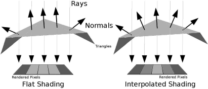
The principle of Gouraud-shading. When rendering a large triangle that is hit by several rays aiming at neighboring pixels in the render plane, we may end up with rather large, dull areas on the rendered image. If the normal vectors for the respective rays are interpolated between the neighboring geometric primitives, we will get a smoother appearance of the rendered surface.
Finally, one may render 2D patterns, so-called textures on the graphic primitives to increase the 3D effect. This is of great importance for instance in computer games, surgical simulation, and other visualization applications. However, in basic medical imaging, textures do usually not play a very important role.
8.4.3 A special application – virtual endoscopy
Finally, a special rendering technique called virtual endoscopy is introduced. An endoscope is an optical instrument with a small wide-angle camera that can be inserted into the body. Various types of flexible and rigid endoscopes for neurosurgery, ENT-surgery and, above all, gastrointestinal interventions exist. It is also possible to take histological samples or to inject drugs using these devices. Given the ergonomics of an endoscope, it is sometimes difficult to orientate oneself during an endoscopic intervention. Therefore it is interesting, for training purposes as well as visualization, to simulate endoscopic views. Since the endoscope is, technically speaking, a wide-angle camera, this can be performed using a perspective surface rendering technique. A special problem here is the simulation of barrel distortion, an optical property of wide-angle lenses that is also known as the fisheye effect. Figure 8.15 shows such a virtual endoscopy – here, we take a look in cranial direction through the cervical spine of our pig CT dataset into the calvaria; the rendering threshold is chosen in such a manner that no soft tissue is visible. Virtual endoscopy has gained some importance in the early detection of colon cancer, where it is sometimes used to generate endoscopy-like views from CT data of the lower abdomen.
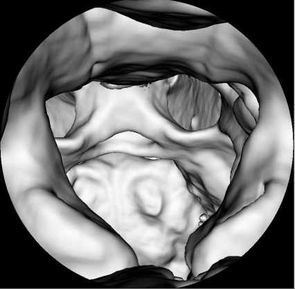
A virtual endoscopy of the spinal canal of the pig dataset, rendered from CT. Basically speaking, this is a surface rendering that, in addition, simulates the barrel distortion induced by the wide angle optics of a conventional endoscope. Image data courtesy of the Dept. of Radiology, Medical University Vienna.
8.5 Practical Lessons
8.5.1 A perspective example
Perspective_8.m illustrates the perspective projection of a cube’s eight cornerpoints. The cube has 10 pixels sidelength. The origin of the cube is located at (10, 10, 0)T. The distance of the viewer, located on the z-axis of the coordinate system is given by fdist. You are encouraged to play with different values of fdist. Some of the possible output can be found in Figure 8.16.
Sample output from Perspective_8.m. As the viewpoint approaches the eight corners of a cube of 10 pixels sidelength, the projection changes from a square to a sheared projection. The first image shows an orthogonal projection since the distance of the viewpoint is 50 times larger than the typical dimension of the object, therefore the projection operator approximates P∞ given in Equation 8.1.
First, we have to the define the cornerpoints of the cube; there is little to be discussed in this part of the script.
1:> clear;
2:> cube=zeros(4,8);
3:> cube(1,1)= 10;
4:> cube(2,1)= 10;
5:> cube(4,1)= 1;
6:> cube(1,2)= 20;
7:> cube(2,2)= 10;
8:> cube(4,2)= 1;
9:> cube(1,3)= 10;
10:> cube(2,3)= 20;
11:> cube(4,3)= 1;
12:> cube(1,4)= 20;
13:> cube(2,4)= 20;
14:> cube(4,4)= 1;
15:> cube(1,5)= 10;
16:> cube(2,5)= 10;
17:> cube(3,5)= 10;
18:> cube(4,5)= 1;
19:> cube(1,6)= 20;
20:> cube(2,6)= 10;
21:> cube(3,6)= 10;
22:> cube(4,6)= 1;
23:> cube(1,7)= 10;
24:> cube(2,7)= 20;
25:> cube(3,7)= 10;
26:> cube(4,7)= 1;
27:> cube(1,8)= 20;
28:> cube(2,8)= 20;
29:> cube(3,8)= 10;
30:> cube(4,8)= 1;
Next, we define an image img to hold the rendering, and the distance of the eyepoint to the viewing plane fdist is being defined. A projection matrix projector is set up as given in Equation 8.2. And we define two vectors to hold the coordinates of the 3D object points and the rendered 2D points.
31:> img=zeros(30,30);
32:> fdist=100;
33:> projector=eye(4);
34:> projector(3,3)=0;
35:> projector(4,3)=-1/fdist;
36:> V=projector;
37:> worldPoints=zeros(4,1);
38:> imagePoints=zeros(4,1);
Finally, we carry out the projection and display the result; denote the renormalization step, which takes care of the different scale of projections in dependence of the distance to the imaging plane:
39:> for j=1:8
40:> for k=1:4
41:> worldPoints(k,1)=cube(k,j);
42:> end
43:> imagePoints=V*worldPoints;
44:> imagePoints=round(imagePoints/(imagePoints(4,1)));
45:> ix=imagePoints(1,1);
46:> iy=imagePoints(2,1);
47:> if (ix > 0 & ix < 30 & iy > 0 & iy < 30)
48:> img(ix,iy)=64;
49:> end
50:> end
51:> colormap(gray)
52:> image(img)
8.5.2 Simple orthogonal raycasting
Raytracing_8.m introduces a very simple version of MIP-rendering using raycasting; there is no perspective involved, therefore all rays are parallel. First, we load a volume that was scaled down and saved with 8 bit depth in order to keep the volume size manageable. The procedure of loading the volume is not new – we know it already from Example 7.6.5:
1:> vol=zeros(98,98,111);
2:> fp = fopen(’pigSmall.img’,’r’);
3:> for z=1:110;
4:> z
5:> for i=1:97
6:> for j=1:97
7:> rho=fread(fp,1,’char’);
8:> vol(i,j,z)=rho;
9:> end
10:> end
11:> end
Next, we introduce a minimum threshold minth for rendering; remember that such a threshold helps to keep the rendered image free from unwanted projections of low-intensity non-zero pixels that may, for instance, stem form the air surrounding the object; a matrix holding the rendered image img is allocated, as well as a vector vox. This vector holds the actual position of the ray passing through the volume:
12:> minth=20;
13:> img=zeros(98,98);
14:> vox=zeros(3,1);
Now we are ready to start the rendering process. The procedure is pretty straightforward; the ray, whose actual position is given in the vox vector proceeds to the volume from a starting point above the volume, following the z-axis. If it hits the image surface, it terminates. A new gray value rho at the actual voxel position beyond the highest gray value encountered so far is assigned the new maximum gray value maxRho if its value is higher than the rendering threshold minth. Once the ray terminates, the maximum gray value is assigned to the rendered image img, and the image is displayed.
15:> for i =1:98
16:> for j =1:98
17:> maxRho=0;
18:> for dep=1:110
19:> vox=transpose([i,j,(110-dep)]);
20:> if vox(1,1) > 0 & vox (1,1) < 98 & vox(2,1) > 0 & vox(2,1) < 98 & vox(3,1)>0 & vox(3,1)<111
21:> rho = vol(vox(1,1),vox(2,1),vox(3,1));
22:> if rho > maxRho & rho > minth
23:> maxRho = rho;
24:> end
25:> end
26:> end
27:> img(i,j)=maxRho;
28:> end
29:> end
30:> minint=min(min(img));
31:> img=img-minint;
32:> maxint = max(max(img));
33:> img=img/maxint*64;
34:> colormap(gray)
35:> image(img)
The – admittedly not very impressive – result is shown in Figure 8.17.

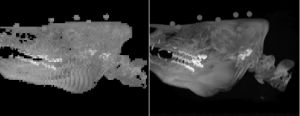
The output from Raytracing_8.m is shown on the left; it shows a frontal MIP rendered from CT data. The image quality is poor because of the small size of the volume; if one uses a more powerful rendering engine like the one of AnalyzeAVW with a volume of better resolution, one gets an image like the one shown on the right. The similarity is, nevertheless, obvious.
Besides the poor resolution, which is atributed to the memory management in MATLAB®, the view is also not very enlightening since we are looking at the snout of our patient. It would be better to rotate the volume around the y-axis so that we get a lateral view. This is, however, not a real problem since we have done this before. RaytracingRotated_8.m does this. It is derived from Raytracing_8.m; the volume is ro-tated, but its boundaries are maintained. The following code is inserted after reading the volume. It rotates the volume – the rotation center is the center of the volume – and writes the result to a volume newvol with the same boundaries as vol. Finally, it copies the rotated volume to vol, and the raycasting algorithm proceeds; the result, together with an equivalent high-quality MIP, is shown in Figure 8.18.
A MIP derived by raytracing, after rotation of the object. A high-quality version with a similar object orientation rendered with AnalyzeAVW can be seen on the right.
...> R=eye(4);
...> R(2,3) = 1;
...> R(3,2) = -1;
...> R(2,2)=0;
...> R(3,3)=0;
...> T=eye(4);
...> T(1,4)=48;
...> T(2,4)=48;
...> T(3,4)=54;
...> invT=inv(T);
...> newvol=zeros(98,98,111);
...> oldvox=zeros(4,1);
...> newvox=zeros(4,1);
...> for i=1:97
...> for j=1:97
...> for z=1:110
...> oldvox(1,1)=i;
...> oldvox(2,1)=j;
...> oldvox(3,1)=z;
...> oldvox(4,1)=1;
...> newvox=round(T*R*invT*oldvox);
...> if newvox(1,1) > 0 & newvox(1,1) < 98 & newvox(2,1) > 0 & newvox(2,1) < 98 & newvox(3,1) > 0 & newvox(3,1) < 111
...> newvol(newvox(1,1),newvox(2,1),newvox(3,1))= vol(i,j,z);
...> end
...> end
...> end
...> end
...> vol=newvol;
Additional Tasks
Inspect the result when changing minth.
Change the script so that it produces a summed voxel rendering instead of a MIP. A possible output can be found in Figure 8.19.

A summed voxel shading rendered with a modified version of Raytra-cing_8.m. The orientation of the volume is similar to Figure 8.18.
8.5.3 Viewpoint transforms and splat rendering
In Splatting_8.m, we implement splatting – the projection of voxels onto the imaging plane using the operator P from Equation 8.1 – as an alternative rendering method. If we just load the volume dataset from Example 8.5.2, the whole code looks like this:
1:> vol=zeros(98,98,111);
2:> fp = fopen(’pigSmall.img’,’r’);
3:> for z=1:110;
4:> for i=1:97
5:> for j=1:97
6:> rho=fread(fp,1,’char’);
7:> vol(i,j,z)=rho;
8:> end
9:> end
10:> end
A MIP rendering using splat rendering looks rather similar to Example 8.5.2. We derive a projection operator P and apply it to all voxel positions vox. If the projected gray value is higher than the one already encountered in the rendering plane img, it replaces the gray value.
11:> img=zeros(98,98);
12:> minth=20;
13:> P=eye(4);
14:> P(3,3)=0;
15:> vox=zeros(4,1);
16:> pos=zeros(4,1);
17:> for i=1:97
18:> for j=1:97
19:> for z=1:110
20:> vox=transpose([i,j,z,1]);
21:> pos=P*vox;
22:> rho=vol(i,j,z);
23:> if pos(1,1) > 0 & pos(1,1) < 98 & pos(2,1) > 0 & pos(2,1) < 98
24:> if rho > img(pos(1,1),pos(2,1)) & rho > minth
25:> img(pos(1,1),pos(2,1)) = rho;
26:> end
27:> end
28:> end
29:> end
30:> end
31:> minint=min(min(img));
32:> img=img-minint;
33:> maxint = max(max(img));
34:> img=img/maxint*64;
35:> colormap(gray)
36:> image(img)
One may ask about the benefit of this approach since the result looks pretty similar to Figure 8.17. The strength of splat rendering as a volume-driven method however lies in the fact that it does not need the whole volume data set. If we load a scaled version of the volume that was used to generate Figure 8.7 with 215 × 215 × 124 = 5731900 voxels and 2 bit depth, we can directly introduce the rendering threshold of -540 HU in the volume and save the volume as a N × 4 matrix; the columns of this matrix consist of the three voxel coordinates and the associated gray value. This vector that still contains most of the gray scale information, has only N = 2579560 columns – these are all the voxels above the rendering threshold. The volume was preprocessed and saved in a file named VoxelVector.dat. Since it is stored as ASCII-text, you can directly inspect it using a text editor. The fact that it was saved as text did, however, blow up the data volume considerably. MATLAB reads this matrix, and a more sophisticated version of Splatting_8.m called BetterSplatting_8.m uses this data, which is loaded in a quick manner. It implements a MIP-rendering routine in only 23 lines of code. First, the matrix VoxelVector.dat is loaded, a projection operator is assigned, and vectors for the 3D voxel coordinates (named vox) and the coordinates on the rendered image (called pos) are allocated:
1:> vect=zeros(2579560,4);
2:> vect=load(’VoxelVector.dat’);
3:> img=zeros(215,215);
4:> P=eye(4);
5:> P(3,3)=0;
6:> vox=zeros(4,1);
7:> pos=zeros(4,1);
Next, we visit each column in the matrix containing the processed volume, which was thresholded at -540 HU; the gray values were shifted in such a manner that the lowest gray value is 0; finally, the resulting rendering is displayed; a selection of possible outputs is presented in Figure 8.20:

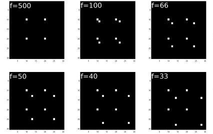
Possible outputs from BetterSplatting_8.m. a shows an orthogonal splat rendering; if a perspective is introduced (in this case, the viewpoint is localized at a distance of 1000 voxels from the imaging plane), the result is Figure b. A translation of t = (-12.7, -12.7, 0, 1)T applied to the perspective projection operator P results in Figure c. A rotation of 90° of the volume gives Figure d. Image data courtesy of the Dept. of Radiology, Medical University Vienna.
8:> for i=1:2579560
9:> vox=transpose([vect(i,1),vect(i,2),vect(i,3),1]);
10:> pos=P*vox;
11:> rho=vect(i,4);
12:> if pos(1,1) > 0 & pos(1,1) < 215 &...pos(2,1) > 0 & pos(2,1) < 215
13:> if rho > img(pos(1,1),pos(2,1))
14:> img(pos(1,1),pos(2,1)) = rho;
15:> end
16:> end
17:> end
18:> minint=min(min(img));
19:> img=img-minint;
20:> maxint = max(max(img));
21:> img=img/maxint*64;
22:> colormap(gray)
23:> image(img)
For the impatient, there is another voxel matrix VoxelVectorBone.dat. It introduces a rendering threshold of 250 HU; only 360562 or approximately 16% of the voxel data are used; applying a perspective summed voxel rendering using this dataset results in Figure 8.21, which is still pretty convincing and is rendered pretty fast compared to Example 8.5.2. Aliasing artifacts, which are basically round-off-errors, become evident here; in more sophisticated approaches these are suppressed by various blurring techniques.4

A summed voxel rendering from the volume VoxelVectorBone.dat, which was preprocessed in such a manner that it only contains the voxels with a gray value of more than 250 HU. Splat rendering can generate a DRR like this from the volume vector in a rather rapid manner. Aliasing artifacts, which are inherent to volume driven approaches and which have to be suppressed by blurring techniques, are, however, clearly visible. Image data courtesy of the Dept. of Radiology, Medical University Vienna.
Additional Tasks
Introduce perspective to BetterSplatting_8.m. Do not forget renormalization of the resulting homogeneous vector.
Change the script BetterSplatting_8.m to implement viewpoint transforms. Start with translations, and compare the effect of the operation TP to PT. Next use small rotations applied to P and comment on the effect.
8.5.4 Volume rendering using color coding
Starting from Example BetterSplatting_8.m, we can modify the script in such a manner that we get a color-coded volume rendering, which resembles the rendering from Figure 8.5.
VolumeSplatting_8.m is the script in question. First of all, we will again clear all variables in the workspace and load our prepared CT-dataset VoxelVector.dat:
1:> clear;
2:> vect=zeros(2579560,4);
3:> vect=load(’VoxelVector.dat’);
Next, we have to assign some memory for three images containing the red, green and blue subimage named imgr, imgg and imgb. If you already forgot about how to compose color image, you may go back to Section 3.2.2:
4:> imgr=zeros(215,215);
5:> imgg=zeros(215,215);
6:> imgb=zeros(215,215);
Now, we will fully utilize our knowledge about spatial transforms to align the volume in such a manner that we look into the eyes of our specimen:
7:> P=eye(4);
8:> P(3,3)=0;
9:> Ry=eye(4);
10:> Ry(1,1)=0;
11:> Ry(1,3)=1;
12:> Ry(3,1)=-1;
13:> Ry(3,3)=0;
14:> Rz=eye(4);
15:> Rz(1,1)=-1;
16:> Rz(2,2)=-1;
What happens here? First, the matrix P is our rendering operator – the projection matrix known from Equation 8.1, which does the orthogonal rendering for us since we are again dealing with a splatting example. Next, we have a rotation matrix Ry, which is the result of a rotation by 270° around the y-axis, as one can verify by inserting this value into Equation 7.13. The next matrix Rz is the result of inserting a value of 180° around the z-axis (see also Equation 7.14). What follows is a translation to make sure that the center of rotation is identical with the center of the center of the volume (see also, for instance, Example 7.6.2); this is matrix T.
17:> T=eye(4);
18:> T(1,4)=107;
19:> T(2,4)=107;
20:> T(3,4)=82;
21:> RM=P*T*Rz*Ry*inv(T);
The one matrix that is finally of interest is the matrix RM; it takes care of rotation for each voxel so that we are “face-to-face” with the dataset instead of looking down on it in a cranio-caudal direction like in some of the images shown in Figure 8.20, it shifts the origin of rotation in an appropriate manner, and the rendering matrix is also in there already. For those who are interested, the full matrix now looks like this:
RM=(00-11890-1021400000001) (8.8)
Next, we assign some memory for the position of the rendered pixel, and we enter a f or-loop that visits each voxel stored in vect, and we apply the matrix RM to the location of the voxel. Finally, the gray value rho associated with each voxel is stored.
22:> pos=zeros(4,1);
23:> for i=1:2579560
24:> pos=RM*(transpose([vect(i,1),vect(i,2) , . . .
vect(i,3),1])) ;
25:> rho=vect(i,4);
What follows is a pretty straightforward routine, which is basically already known, for instance, from Example 8.5.2. We carry out a DRR-rendering (see also Equation 8.4). After taking care that the rendered pixels are within the range of the images imgr, imgg and imgb, we render
a voxel with a gray value between 250 and 1250 into imgr - therefore all soft tissue with a Hounsfield-density below 226 will be rendered as a red pixel. Denote that the volume contained in VoxelVector.dat was shifted in intensity from the Hounsfield scale to an unsigned 12 bit range, therefore the rendering threshold 250 corresponds to -774 HU.
a voxel with gray value between 1250 and 1750 into imgr and imgg. Voxels in this intensity range are rendered as yellow pixels.
a voxel with a gray value above 1750 (which is equivalent to a Hounsfield density of 726) into all three images. These voxels will be displayed as white pixels.
In fact, we implement a very simple version of a transfer function as shown in Figure 8.6 in this case.
26:> if pos(1,1) > 0 & pos(1,1) < 215 & pos(2,1) > 0 & pos(2,1) < 215
27:> if (rho > 250) & (rho < 1250)
28:> imgr(pos(1,1),pos(2,1))=imgr(pos(1,1),...
pos(2,1))+rho;
29 :> end
30:> if (rho >= 1250) & (rho < 1750)
31 :> imgr(pos(1,1),pos(2,1))=imgr(pos(1,1),...
pos(2,1))+rho;
32:> imgg(pos(1,1),pos(2,1))=imgg(pos(1,1),...
pos(2,1))+rho;
33:> end
34:> if (rho >= 1750)
35:> imgr(pos(1,1),pos(2,1))=imgr(pos(1,1),...
pos(2,1))+rho;
36:> imgg(pos(1,1),pos(2,1))=imgg(pos(1,1),...
pos(2,1))+rho;
37:> imgb(pos(1,1),pos(2,1))=imgb(pos(1,1),...
pos(2,1))+rho;
38:> end
39:> end
40:> end
After the image is rendered, we have to scale the three color channels imgr, imgg and imgb to an intensity range from 0 ... 1, which is the common representation for color. You may also recall Example 4.5.2, where we did something similar. However, we do not have to assign a lookup table using the colormap routine when displaying such an RGB-image. Beyond that, we know that our volume is saved as unsigned 16 bit values. Therefore, we can also omit the usual step of subtracting the minimum grayvalue prior to scaling the intensity range.
41:> maxint = max(max(imgr));
42:> imgr=imgr/maxint;
43:> maxint = max(max(imgg));
44:> imgg=imgg/maxint;
45:> maxint = max(max(imgb));
46:> imgb=imgb/maxint;
Finally, we have to insert the single color channel images into one RGB-color image, and this image is displayed. The result (whose color version can be found on the accompanying CD), is shown in Figure 8.22.
The output from the script VolumeSplatting_8.m, a color-coded volume rendering similar to Figure 8.5. The original MATLAB output is in color. Again, for the sake of keeping the printing cost within reasonable limits, we print this image in grayscale. However, the color version can be found on the accompanying CD. Image data courtesy of the Dept. of Radiology, Medical University Vienna.
47:> colorimg=zeros(215,215,3);
48:> for i=1:215
49:> for j=1:215
50:> colorimg(i,j,1)=imgr(i,j);
51:> colorimg(i,j,2)=imgg(i,j);
52:> colorimg(i,j,3)=imgb(i,j);
53:> end
54:> end
55:> image(colorimg)
Our example is somewhat simplistic – we do not really use subtleties such as opacity or voxel location to create our image. However, you may compare this image to a grayscale image that is generated by simple summed voxel shading without color coding.
Additional Tasks
Draw a graph of the intensity transfer function for this example similar to Figure 8.6.
8.5.5 A simple surface rendering - depth shading
Based on Splatting_8.m, we can also introduce the most simple of all surface rendering techniques - depth shading, introduced in Figure 8.7; here, a transfer function TDS as given in Equation 8.5 is used. What looks complicated at a first glance is actually pretty simple; for all voxels with coordinates →x on a ray aiming at the pixel →xImage Plane, we determine the maximum gray value to be proportional to the voxel with the largest distance to the image plane. In other words: voxels far away from the image plane are brighter than voxels close to the image plane.
To some extent, depth shading is pretty similar to MIP. But it does not determine a gray value from the content of the volume to be rendered but from the geometrical properties of the voxels relative position to the image plane. To some extent, depth shading is a little bit similar to the distance transform, introduced in Section 5.3.2.
Let’s take a look at the code; in the script DepthShading_8.m, the volume is read and the volume transform matrix is set up, just as we did in Splatting_8.m; here, we do not shift the projection operator, but we transform the origin of volume rotation prior to rendering:
1:> vect=zeros(360562,4);
2:> vect=load(’VoxelVectorBone.dat’) ;
3:> img=zeros(215,215);
4:> P=eye(4);
5:> P(3,3)=0;
6:> vox=zeros(4,1);
7:> pos=zeros(4,1);
8:> R=eye(4);
9:> R(1,1)=0;
10:> R(1,3)=1 ;
11:> R(3,1)=-1 ;
12:> R(3,3)=0;
13:> T=eye(4);
14:> T(1,4)=107;
15:> T(2,4)=107;
16:> T(3,4)=82;
17:> invT=inv(T);
The only difference to Splatting_8.m is implemented here. We rotate each voxel in the appropriate position, compute the projected position, and determine the gray value rho as the absolute value of the z-coordinate in the 3D voxel position. This is equivalent to the distance of the voxel to the image plane since our projection operator P is set up in such a manner that it splats all voxels to the x-y plane of the volume coordinate system. Next, we check whether another rendered voxel has a higher intensity (and therefore stems from a position at a greater distance to the rendering plane); if this is not case, the gray value is stored at the pixel position, just as we did in Examples 8.5.2 and 8.5.3 when rendering MIPs. Finally, the result is displayed like so many times before:
18:> for i=1:360562
19:> vox=T*R*invT*...
(transpose([vect(i,1),vect(i,2),vect(i,3),1]));
20:> pos=P*vox;
21:> rho=abs(vox(3,1));
22:> if pos(1,1) > 0 & pos(1,1) < 215 & pos(2,1) > 0 & pos(2,1) < 215
23:> if rho > img(pos(1,1),pos(2,1))
24:> img(pos(1,1),pos(2,1)) = rho;
25:> end
26:> end
27:> end
28:> minint=min(min(img));
29:> img=img-minint;
30:> maxint = max(max(img));
31:> img=img/maxint*64;
32:> colormap(gray)
33:> image(img)
The result, which is very similar to Figure 8.7, can be found in Figure 8.23. Depth shading is not a very sophisticated surface rendering technique, but is useful for simple rendering tasks, and it directly leads us to surface rendering using voxel surface, which will be explored in Example 8.5.6.
The output of DepthShading_8.m, where a depth shading is computed using a splat rendering technique. For your convenience, this illustration was rotated by 180°compared to the original image as displayed by DepthShading_8.m. Image data courtesy of the Dept. of Radiology, Medical University Vienna.
Additional Tasks
Depth shading assigns a brightness to each surface voxel in dependence of its distance to the viewer. Therefore, the lighting model of depth shading is similar to a setup where each surface voxel glows with the same intensity. The intensity of a point light source in dependence of the viewers distance, however, follows the inverse square law – it decreases in a quadratic fashion. A physically correct depth shading method would therefore map the square of the distance between surface voxel and viewpoint. Can you modify DepthShading_8.m in such a fashion that it takes this dependence into account? The result can be found in Figure 8.24.

If one takes the lighting model of depth shading seriously, it is necessary to apply the inverse square law to the brightness of each surface voxel – the brightness of a surface voxel therefore depends on the square of the distance to the viewpoint. A small modification in DepthShading_8.m takes this into account; the result is, however, not very different from the simple implementation with a linear model, shown in Figure 8.23. Image data courtesy of the Dept. of Radiology, Medical University Vienna.
8.5.6 Rendering of voxel surfaces
In SurfaceShading_8.m, we expand the concept of depth shading to render more realistic surfaces. For this purpose, we go back to orthogonal raycasting and apply a simple flat shading model to a volume already segmented using a simple thresholding operation; again, we will use a volume of the skull CT. A threshold was introduced in such a manner that it only contains voxels with binary values. Only the bone remains here. This time, the non-zero voxels are stored in a file containing an N × 3 matrix named VoxelVectorThreshold.dat. The non-zero voxel coordinates are read, rotated to the same position as in Example 8.5.5, and stored in a 215 × 215 × 215 volume vol.
1:> vect=zeros(360562,3);
2:> vect=load(’VoxelVectorThreshold.dat’);
3:> vol=zeros(215,215,215);
4:> vox=zeros(3,1);
5:> R=eye(4);
6:> R(1,1)=0;
7:> R(1,3)=1;
8:> R(3,1)=-1;
9:> R(3,3)=0;
10:> T=eye(4);
11:> T(1,4)=107;
12:> T(2,4)=107;
13:> T(3,4)=62;
14:> invT=inv(T);
15:> for i=1:360562
16:> vox=round(T*R*invT*... (transpose([vect(i,1),vect(i,2),vect(i,3),1])));
17:> if vox(1,1) > 0 & vox(1,1) < 216 & ... vox(2,1) > 0 & vox(2,1) < 216 & vox(3,1) > 0 & ... vox(3,1) < 216
18:> vol(vox(1,1),vox(2,1),vox(3,1)) = 1;
19:> end
20:> end
Now we have a volume, and we can apply a raycasting technique just as we did in Example 8.5.2. The difference lies in the way we assign a gray value to the new intermediate image called hitmap. We proceed along a beam which is parallel to the z-axis towards the imaging plane by an increment dep; if a non-zero voxel is encountered in vol, the ray is clipped, and the z-coordinate is stored in hitmap. If the ray does not encounter a voxel, it is terminated once it reaches the x-y-plane of the coordinate system. Figure 8.25 shows a surface plot of hitmap.

The surface representation of hitmap, generated using MATLAB’s surf function. hitmap stores the z-coordinate when a beam hits a voxel surface of the volume vol. Based on this data, a surface normal is computed, and a lighting model can be applied. Basically speaking, the surf function already does this. Image data courtesy of the Dept. of Radiology, Medical University Vienna.
21:> hitmap=zeros(215,215);
22:> img=zeros(215,215);
23:> for i=1:215
24:> for j=1:215
25:> hit=0;
26:> dep=215;
27:> while hit == 0
28:> if vol(i,j,dep) > 0
29:> hit=1;
30:> hitmap(i,j)=dep;
31:> end
32:> dep=dep-1;
33:> if dep < 1
34:> hit=1;
35:> end
36:> end
37:> end
38:> end
The next step is to apply a lighting model. For this purpose, we have to compute the normal vector on every surface voxel we already encountered. In order to do so, we have to allocate memory for a few vectors:
39:> normal=zeros(3,1);
40:> beam=transpose([0,0,1]) ;
41:> gradx=zeros(3,1);
42:> grady=zeros(3,1);
normal will become the normal vector. beam is the unit vector in the direction of the ray, which proceeds parallel to the z-axis towards the image plane. gradx and grady are two gradients in x- and y-direction - see also Figure 8.9 for an illustration. These are computed as finite differences between the neighboring pixels of a pixel at position →x=(i,j)T in hitmap.
However, these gradients are three-dimensional; they are given by the 2D coordinate of a surface voxels projection in the planar image hitmap and the z-value stored in hitmap. The gradient in x-direction as a finite difference (remember Chapter 5) is given as:
gradx=∇(ijhitmap(i,j))=(i+1jhitmap(i+1,j))−(i−1jhitmap(i−1,j)) (8.9)
grady is computed in a similar way. The surface normal, normal, is the outer or cross-product of gradx and grady. In MATLAB, this product is computed by calling the function cross. In order to determine the tilt of the surface relative to the beam, we compute the inner product of normal and beam. Remember Chapter 5 - in a Cartesian coordinate system, the inner product of two vectors is given as →a•→b=||→a|| ||→b||cos (α) where α is the angle enclosed by the two.
Our lighting model is simply given by an ambient light that is reflected according to the cosine of its angle of incidence - see Equation 8.6. Here, the light beam is identical to the view direction beam (just like a headlight). The inner product, computed in MATLAB by calling dot, of the normal vector normal, scaled to length 1, and beam gives us the amount of reflected light. Let’s take a look at the code:
43:> for i =2:214
44:> for j =2:214
45:> if hitmap(i,j) > 1
46:> gradx=transpose([(i+1),j,hitmap((i+1),j)]) - transpose([(i-1),j,hitmap((i-1),j)]);
47:> grady=transpose([i,(j+1),hitmap(i,(j+1))]) - transpose([i,(j-1),hitmap(i,(j-1))]);
48:> normal=cross(gradx,grady) ;
49:> refl=dot(normal,beam)/(norm(normal)) ;
50:> img(i,j) = 64*refl;
51:> end
52:> end
53:> end
54:> colormap(gray)
55:> image(img)
Here, we do just as told. The cross-product of the x- and y-gradients gives us the normal to the surface segment defined by the non-zero voxel encountered by the ray aiming at the image plane and its direct neighbors. The inner product of beam and normal gives a value between 1 and zero. Multiplying the maximum intensity by the cosine gives us an image intensity between 0 and 64. This can be directly displayed. We don’t want to render the image plane itself, therefore only positions in hitmap larger than one are taken into account. Figure 8.26 shows the result of SurfaceShading_8.m.
The result of SurfaceShading_8.m. By using a simple lighting model, which is actually the cosine of an incident ray of light parallel to the ray cast through the volume and the surface normal, we get a surface rendering from a segmented binary voxel volume. Image data courtesy of the Dept. of Radiology, Medical University Vienna.
Additional Tasks
Plot hitmap instead of img. Does the output look familiar?
Can you change the appearance of the image by varying the light? It is actually just one line of code; a possible result is shown in Figure 8.27.
Some possible results from the additional tasks; in a. a different visualization of the volume data set is achieved by changing the direction of the incoming light. In b, a perspective surface shading is generated from depth shading derived in Example 8.5.5. The artifacts already visible in Figure 8.21 become even more prominent since no countermea-sures against aliasing are taken. Image data courtesy of the Dept. of Radiology, Medical University Vienna.
Once you have mastered the first task here, it is pretty straightforward to combine DepthShading_8.m and SurfaceShading_8.m to produce a perspective surface rendering. Can you think of a simple method to reduce the aliasing artifacts visible in Figure 8.27? Alternatively, one can also implement perspective raycasting. In such a case, all rays proceed from the eyepoint to a pixel on the render plane.
8.5.7 A rendering example using 3DSlicer
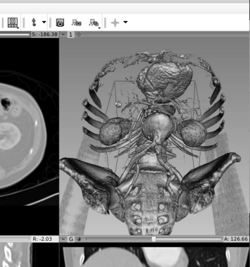
Of course, we can also explore the possibilities of the 3D visualization also by means of 3DSlicer. For this purpose, one can for instance simply download a sample dataset by pressing the button “Download Sample Data” in the startup screen; in Fig. 8.28, we see the dialog which allows for downloading sample datasets. In the given case, a CT dataset of the abdominal region (called “CTAbdomen” in the module Sample Data) was loaded. On this dataset, one can try various visualization options. However, it makes sense to use a CT since the good contrast of bone compared to soft tissue allows for a decent visualization.

When clicking the module “Sample Data” in 3DSlicer, one can download a number of datasets for demonstration purposes. For rendering, it makes sense to try a CT dataset first since the high contrast of bone allows for simple segmentation and visualization. In this case, the dataset “CTAbdomen” was loaded. After finishing the download, the main screen of 3DSlicer should resemble this illustration.
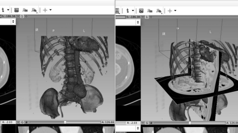
Next, one should switch to the module “Volume Rendering”, which can be selected in the uppermost menu on the main screen. Next, the rendering has to be made visible using the “eye icon” in the left menu, and by selecting a preset, for instance “CT-AAA” in the pull-down menu “Display”. Fig. 8.29 shows the looks of this setup in Slicer 4.2.2-1.
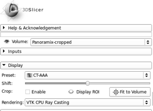
The settings for displaying a volume rendering in 3DSlicer Ver. 4.2.2. The result can be found in Fig. 8.30.
By rolling the mouse wheel and by moving the mouse with the left mouse button pressed, one can manipulate the view of the rendering. Choosing different volume rendering presets will also result in different views - Fig. 8.30 gives an example.
By switching to the display preset “CT-Bones” and by making the sincle slices “visible” (via the “eye icon” in the submenus of the single CT-slices), one can also show the spatial orientation of the reformatted images in the rendering (see also Fig. 8.31).
A rendering from 3DSlicer with the “CT-Bones” preset, with and without the slices from the orthogonal views visible.
8.5.8 Extracting a surface using the cuberille algorithm
In Triangulation_8.m, we find a very simple implementation of a surface triangulation technique referred to as the cuberille algorithm. It simply assigns a rectangle (or, in our case, two triangles forming a rectangle) to every voxel surface in a segmented binary volume that does not have a neighbor. The volume data of a segmented pedicle are stored as coordinate triplets in a simple text file named PedicleSegmented.dat in the LessonData folder. It consists of 16922 coordinates for non-zero voxels. The file is written in plain text, and you can inspect it using a simple text editor. Since indices in MATLAB start with 1 instead of 0, we have to add one to each coordinate; this results in a vector pos, which is stored in a 59 × 57 × 27 volume named vol:
1:> vect=zeros(16922,3);
2:> vect=load(’PedicleSegmented.dat’);
3:> pos = zeros(3,1);
4:> vol=zeros(60,58,27);
5:> for i=1:16922
6:> pos(1,1)=round(vect(i,1))+1;
7:> pos(2,1)=round(vect(i,2))+1;
8:> pos(3,1)=round(vect(i,3))+1;
9:> vol(pos(1,1),pos(2,1),pos(3,1))=1;
10:> end
Next, we remove all stray voxels (this is the voxels that don’t have any neighbors) for the sake of simplicity. We are also not interested in the voxels that have six nearest neighbors since these cannot be part of a surface; the result of this operation is stored in a new volume named cleanvol:
11:> cleanvol=zeros(60,58,27);
12:> for i=2:59
13:> for j=2:57
14:> for k=2:26
15:> if vol(i,j,k) > 0
16:> noOfNeighbors=vol(i+1,j,k)+vol(i-1,j,k)+ vol(i,j+1,k)+vol(i,j-1,k)+vol(i,j,k+1)+vol(i,j,k-1);
17:> if (noOfNeighbors > 0) & (noOfNeighbors <= 5)
18:> cleanvol(i,j,k) = 1;
19:> end
20:> end
21:> end
22:> end
23:> end
Now, we can assign triangles to every surface without a neighbor; since visualization of triangulated models is a rather widespread problem, a large number of viewers is available, and therefore we do not show the result of our efforts, but rather than that we save the list of triangles in an ASCII-encoded STL-file named PedicleSurface.stl. In order to identify the neighbors, we also define three unit vectors evecx, evecy, and evecz. By consecutively subtracting and adding these unit vectors to a non-zero voxel position voxvec, we can scan all six nearest neighbors of this voxel. If the result resvec of this simple computation – the subtraction and addition of the unit vectors – is zero, we find a surface, and this face of the voxel is stored as two triangles in the STL-file. The total number of triangles is stored in a counter variable named trianglecount. We only show the first of six such computations – the remaining five are similar:
24:> fp=fopen(’PedicleSurface.stl’,’w’);
  25:> fprintf(fp,’solid PedicleSurface
’);
26:> evecx=transpose([1,0,0]);
27:> evecy=transpose([0,1,0]);
28:> evecz=transpose([0,0,1]);
29:> voxvec=zeros(3,1);
30:> resvec=zeros(3,1);
31:> trianglecount = 0;
32:> for i=2:59
33:> for j=2:56
34:> for k=2:26
35:> if cleanvol(i,j,k) > 0
36:> voxvec(1,1)=i;
37:> voxvec(2,1)=j;
38:> voxvec(3,1)=k;
39:> resvec=voxvec-evecx;
40:> if cleanvol(resvec(1,1),resvec(2,1), resvec(3,1)) == 0
  41:> fprintf(fp,’facet normal 0.0 0.0 0.0
’);
  42:> fprintf(fp,’outer loop
’);
  43:> vertexstring=sprintf(’vertex %f %f %f
’, double(i),double(j),double(k));
44:> fprintf(fp,vertexstring);
  45:> vertexstring=sprintf(’vertex %f %f %f
’, double(i),double(j+1),double(k));
46:> fprintf(fp,vertexstring);
  47:> vertexstring=sprintf(’vertex %f %f %f
’, double(i),double(j),double(k+1));
48:> fprintf(fp,vertexstring);
  49:> fprintf(fp,’endloop
’);
  50:> fprintf(fp,’endfacet
’);
  51:> fprintf(fp,’facet normal 0.0 0.0 0.0
’);
  52:> fprintf(fp,’outer loop
’);
  53:> vertexstring=sprintf(’vertex %f %f %f
’, double(i),double(j+1),double(k));
54:> fprintf(fp,vertexstring);
  55:> vertexstring=sprintf(’vertex %f %f %f
’, double(i),double(j+1),double(k+1));
56:> fprintf(fp,vertexstring);
  57:> vertexstring=sprintf(’vertex %f %f %f
’, double(i),double(j),double(k+1));
58:> fprintf(fp,vertexstring);
  59:> fprintf(fp,’endloop
’);
  60:> fprintf(fp,’endfacet
’);
61:> trianglecount=trianglecount+2;
62:> end
...
...:> end
...:> end
...:> end
...:> end
...:> trianglecount
  ...:> fprintf(fp,’endsolid PedicleSurface
’);
...:> fclose(fp);
Next, we should take a look at the result of our efforts; for this purpose, we need a viewer for surface models. A very powerful freeware software for this purpose is ParaView, a joint effort of Kitware5 Inc. and several national laboratories in the United States. Paraview can simply be downloaded and started; other viewer applications such as Blender are also available in the public domain. Once we’ve loaded the PedicleSurface.stl into Paraview and all parameters are computed, we can inspect our model from all sides; a possible result can be found in Figure 8.32.

The result of our humble cuberille triangulation algorithm implemented in Triangulation_8.m, saved in PedicleSurface.stl; the screenshot was taken from ParaView. The blocky appearance is an inevitable result of the cuberille algorithm that simply assigns two triangles to every visible voxel surface. Image data courtesy of the Dept. of Radiology, Medical University Vienna.
Additional Tasks
In the LessonData folder, you may find a binary STL-file named PedicleSmooth.stl. This file was generated using a Marching Cubes method with variable cube size. Inspect it using your STL-viewer and compare the looks to PedicleSurface.stl. A possible output can be found in Figure 8.33.

The result of rendering PedicleSmooth.stl, a surface model of the same pedicle as in Figure 8.32, generated by a more sophisticated algorithm based on the Marching Cubes algorithm implemented in AnalyzeAVW. Image data courtesy of the Dept. of Radiology, Medical University Vienna.
8.5.9 A demonstration of shading effects
If you have done your homework in Example 8.5.6 properly, you might already have noticed that the hitmap image is nothing but a depth shading. Since the position of the first surface voxel is encoded in this 2D-image, we can derive the 3D gradients spawning the normal vector and generate a realistic surface rendering from this information. However, we have used flat shading. The illumination of every voxel is simulated from its 2D counterpart in hitmap. Given the fact that our volume is rather coarse, the result as shown in Figure 8.26 is blocky and does not look very attractive. For this reason, we may apply a more sophisticated shading model similar to Gouraud- or Phong-shading. As we have learned from Section 8.4, we have to interpolate either the grid of normal vectors or the color of the shading to get a smooth appearance. We will implement such a technique (which is not exactly equivalent to the aforementioned shading algorithms, but illustrates the way these work) by manipulating hitmap. Therefore we have to run BetterShadingI_8.m, which is derived from SurfaceShading_8.m; this script saves hitmap as a .PGM file as we already did in Example 3.7.2 and terminates without rendering; the first part of the script is copied from SurfaceShading_8.m until hitmap is generated; the hitmap image is stored in a PGM file named IntermediateHitmap.pgm, which can be opened using GIMP or another standard image processing program like Photoshop:
...:> pgmfp = fopen(’IntermediateHitmap.pgm’,’w’);
  ...:> str=sprintf(’P2
’);
...:> fprintf(pgmfp,str);
  ...:> str=sprintf(’215 215
’);
...:> fprintf(pgmfp,str);
...:> maximumValue=max(max(hitmap))
  ...:> str=sprintf(’%d
’,maximumValue);
...:> fprintf(pgmfp,str);
...:> for i=1:215
...:> for j=1:215
...:> str=sprintf(’%d ’,hitmap(i,j));
...:> fprintf(pgmfp,str);
...:> end
...:> end
...:> fclose(pgmfp);
We can now do everything we need to get a better rendering in GIMP. The single steps to be carried out are as follows:
Rotate the image by 180° in order to provide an image that is not displayed heads-up.
Interpolate the image to a larger image size. In order to generate the renderings given in Figure 8.35, the image was cropped and scaled to 900 × 729 pixels using cubic interpolation.
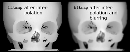
hmap.pgm and hmapblurred.pgm; these images are generated from the hitmap image from BetterShadingI_8.m by carrying out the interpolation and blurring steps from Example 8.5.9. A surface rendering of these images results in Figure 8.35. Image data courtesy of the Dept. of Radiology, Medical University Vienna.
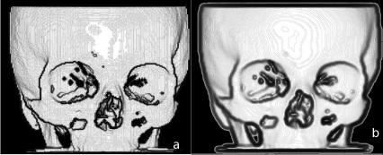
Additional interpolation of shading effects such as Gouraud- and Phong shading improve the appearance of a rendered model further. This rendering was generated using the same data as in Figure 8.26. However, the appearance is smoother and less blocky thanks to a manipulation of the hitmap image. The manipulations we applied to the intermediate depth shading IntermediateHitmap.pgm somewhat resemble Phong-shading. Image data courtesy of the Dept. of Radiology, Medical University Vienna.
The interpolation already provides some type of low-pass filtering; we can emphasize this by adding an additional blurring using a 5×5 Gaussian blur kernel. By doing so, we distribute the gray values in a smooth manner; the gradients computed from this smoothed image are smoothed as well, and this provides the shading effect.
The resulting image is stored again, this time as a binary PGM. Such a PGM has starts with P5, as you may recall from Chapter 3. The header is 54 bytes long. If you run into trouble saving the smoothed IntermediateHitmap.pgm file, you may as well use the pre-generated image files hmap.pgm and hmapblurred.pgm files provided in the LessonData/8_Visualization folder in the following BetterShadingII_8.m script. hmap.pgm and hmapblurred.pgm are shown in Figure 8.34. You can, of course, also use the scripts from Examples 7.6.2 and 5.4.1 to achieve the same effect.
The modified hitmap images are now rendered in a second script named BetterSha-dingII_8.m; loading the binary PGM files hmap.pgm and hmapblurred.pgm is carried out similar to Example 3.7.2. The PGM header is 54 bytes long and is skipped:
...:> fp=fopen(’hmap.pgm’,’r’);
...:> hitmap=zeros(900,729);
...:> fseek(fp,54,’bof’);
...:> hitmap(:)=fread(fp,(900*729),’uint8’);
...:> hitmap=transpose(hitmap);
...:> fclose(fp);
The remainder of the script applies a surface rendering routine on the 900×729 image; it is directly copied from Example 8.5.6. The result can be found in Figure 8.35. A significant improvement in image quality could be expected if we use a finer voxel resolution than the 1 × 1 × 1mm3 dimension used in the VoxelVectorThreshold.dat volume. However, the shading technique used here is some sort of trick; we use the depth shading to compute the 3D gradients as we did before in Example 8.5.6. By interpolation, we increase the number of rays aiming at the rendering plane, and the gradients to be computed are interpolated by the blurring step.
Additional Tasks
Why does this example resemble a Phong-shading? At least we are interpolating gray values in the rendered image, which is the principle of Gouraud shading!
What happens if one applies an intensity scaling operation to IntermediateHit-map.pgm?
8.6 Summary and Further References
Rendering is an important tool for conveying information; in clinical practice, it is mainly appreciated by non-radiologists, who are usually not trained to a great extent to retrieve diagnostic information from slices. Still, the most important visualization techniques from a diagnostic point of view remain windowing and reformatting rather than rendering. Volume rendering, which in many cases does not require an explicit segmentation step, deserves special consideration for such visualization tasks. Surface rendering from voxel surfaces or triangulated meshes does require segmentation and may furthermore suffer from geometrical inaccuracy. Still, it is an important tool for fast visualization and the production of tangible models using rapid prototyping. In practice, one usually does not have to develop a rendering or triangulation algorithm from scratch since these are available as well-tested and widespread application programmers interfaces.
Literature
J. D. Foley, A. van Dam, S. K. Feiner, J. F. Hughes: Computer Graphics: Principles and Practice in C, Addison-Wesley (1995)
J. K. Udupa, G. T. Herman: 3D Imaging in Medicine, Second Edition, CRC Press, (2000)
B. Preim, D. Bartz: Visualization in Medicine, Morgan-Kaufmann, (2007)
M. Hadwiger, J. M. Kniss, C. Rezk-Salama, D. Weiskopf: Real-time Volume Graphics, A. K. Peters, (2006)
R. S. Wright, B. Lipchak, N. Haemel: OpenGL SuperBible: Comprehensive Tutorial and Reference, Addison-Wesley (2007)
W. Schroeder, K. Martin, B. Lorensen: Visualization Toolkit: An Object-Oriented Approach to 3D Graphics, Kitware, (2006)
1A synonymous term is raytracing; we encountered this method earlier, in Chapter 5, where the imaging behavior of a spherical mirror was simulated using a raytracing software for optical design.
2This refers to the fact that the location of the voxel determines the position of a pixel in the rendering. It must not be confused with volume rendering.
3If you already forgot about connectedness, you may take a quick look at Figure 5.9.
4An example for an efficient blurring technique can be found in W. Birkfellner, R. Seemann, M. Figl et al. Wobbled splatting–a fast perspective volume rendering method for simulation of x-ray images from CT, Phys Med Biol, 50(9):N73-84, (2005).
5Kitware is also the home of the heroes that brought us such splendid things as VTK, ITK, and IGSTK. Their homepage is www.kitware.com.