
Chapter 6
Segmentation
Wolfgang Birkfellner
6.1 The Segmentation Problem
We have already learned that medical images map certain physical properties of tissue and store the resulting discrete mathematical function as an image. It is a straightforward and understandable desire that anyone who uses medical images wants to identify certain anatomical structures for further examination; identifying organs or other anatomical structures is an inevitable prerequisite for many operations that retrieve quantitative data from images as well as many visualization tasks.
Unfortunately, physical properties of tissue as recorded by a medical imaging device do usually not correlate completely with the anatomic boundaries of certain organs. That is a very fundamental problem since most organs do not consist of one type of tissue. Segmentation is therefore always a rather complex, specialized procedure often requiring considerable manual interaction, which renders image processing methods requiring segmentation to be quite unattractive. The need for highly specialized solutions is also documented by the plethora of research papers, which usually present rather specialized techniques for a certain type of application. The following chapter introduces the most basic segmentation methods, which usually are the basis for more complex approaches.
6.2 ROI Definition and Centroids
The easiest way to identify a region on an image is to draw an area that defines the region-of-interest (ROI) and to evaluate gray values ρ only within that ROI. This method is by no means automatic, but does nevertheless play an important role for many practical applications. The selection of the rectangular signal-free area for Example 3.7.5 is a classical example for a ROI. An automatic registration algorithm delineating a certain area or volume within an image does also provide a ROI. Usually it is planned that the ROI coincides with the anatomical region of interest as a result of the segmentation procedure. However, in certain imaging modalities, a ROI can also consist of a more general bounding box, where the remainder of the segmentation can be done by selecting intensities. A typical example is ROI selection in nuclear medicine, where absolute count rates, giving a measure of metabolic activity, may be of greater interest than anatomical detail connected to that region of the body. Section 6.8.1 gives a very simple example of such a procedure.
Connected to any ROI is also the centroid of this very region. The centroid of a ROI is usually defined as a central point that gives a reference position for that ROI. Throughout this book, we will encounter the centroid in several occasions, for instance if a precise figure for the position of an extended structure such as a spherical marker is required, or if a reference position for decoupling rotation and translation of point clouds is required. More on this topic can be found in Section 9. In general, a centroid is computed as the average vector of all vectors of the ROI-boundary:
For a symmetrical ROI like a segmented fiducial marker of spherical shape, this centroid is also the most accurate estimate for the marker’s position. However, if the ROI is not given by a boundary, but by an intensity region, the vectors pointing at the pixels which are part of the ROI are to be weighted with their actual gray value before they are summed up.
6.3 Thresholding
The tedious process of drawing ROIs in images – especially if they are given in 3D – can be simplified by algorithms. Here, the ROI is defined by the segmentation algorithm. While the outcome of an image is usually a binary mask that delineates a ROI, we should be aware that such a mask can of course be used to remove unwanted parts outside the ROI of a grayscale image. If the ROI is given in a binary manner, a component-wise multiplication (see also Section 3.1.1) of the ROI mask (consisting of values 0 and 1) achieves this. In Figure 6.15, you can see such an image containing the grayscale information inside the ROI only.
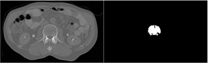
The most basic approach is to divide the image in areas that contain interesting information vs. areas that are not interesting by making a binary classification based on gray levels. One knows, for instance from Table 4.1, that bone usually exhibits an image density ρ above 50 HU. A very basic approach towards segmentation is to get rid of all voxels which have a density ρ below that value. This process is called thresholding. When performing a thresholding operation, a binary model of voxels is built. Figure 6.1 shows a segmentation result for an axial slice from a multislice CT scan of a heart. The volume was acquired at an early phase after injection of contrast agent. The left ventricle, the atrium, and the aorta show excellent contrast.
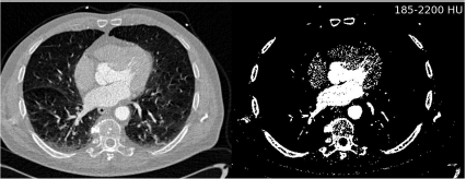
A segmentation example on a CT slice of the human heart. By defining an appropriate threshold, a binary image is created. The binary image contains, besides the bone and the contrast enhanced part of the heart, also parts of some large vessels in the lung and parts of the patient table. A full segmentation of the heart (or of parts of it containing contrast agent) without these additional structures is not possible by thresholding. Image data courtesy of the Dept. of Radiology, Medical University Vienna.
Usually, all gray scale information is lost and replaced by binary values, which automatically define a ROI. Another example is given in Figure 6.2, where a CT-scan of a patient’s abdomen is thresholded, and subsequently, a rendering (a photo realistic visualization from the thresholded CT volume – see Chapter 8) of the thresholded volume was made using Analyze AVW.

Eight rendered images of an abdominal CT-scan which underwent thresholding at different levels of the minimum image intensity. The first rendering was taken from the volume when setting the threshold to -1000 HU. The renderer displays the surface of the binary volume. Here, this is the shape of a cylinder. The threshold is so low that the air surrounding the patient in the CT was not removed. At a threshold of -900 HU, we see the blanket covering the patient. -300 HU is obviously a sufficient threshold to remove the blanket so that the skin of the patient becomes visible. The last image in the upper row was made at a threshold of 0 HU - the radioopacity of water. Part of the skin is now removed, and part of the musculoskeletal system becomes available. At 100 HU, large parts of the musculature are removed. The bladder containing contrast agent becomes visible, and so does part of the digestive system. At 300 HU, the bladder no longer gives sufficient contrast, but the renal system and the bones do. At 500 HU, we still see the renal system. Bone with lesser density is also removed. At 1000 HU, only the cortical bone remains. Image data courtesy of the Dept. of Radiation Oncology, Medical University Vienna.
In Figure 6.2, we see a lot of information, but none of these visualizations is very convincing. At no point in time do we see a particular part of the organs completely exposed. At lower thresholds, a mixture of soft tissue, contrast agent, and bone is visible. At higher thresholds, the bone with lesser density disappears, revealing quite ugly holes in the volume. A straightforward approach would be to apply an intensity transform that emphasizes the structure of interest, and to apply thresholding afterwards. Unfortunately, the diversity in man is so great that this only works to a very limited extent. Keep in mind that we are imaging physical properties of tissue, we are not taking images of organs. Therefore it cannot be excluded that two types of tissue have the same density. It is also a matter of fact that a certain type of tissue does not have one and only one type of radioopacity, but rather than that, a range in densities is covered. Things do even become more complicated when modalities with excellent soft tissue contrast such as MR are used. Here, a naive thresholding approach is bound to fail by nature.
A possibility to make thresholding a more sophisticated method is local thresholding; instead of defining a global threshold, which determines whether a pixel (or voxel) belongs to a given structure, one can also define a window around the local average gray value within a defined area. In short, a local thresholding algorithm consists of
the definition of a typical area (typically a circle with given radius, or a rectangle), in which the average gray value is calculated.
the definition of a local threshold (or a pair consisting of an upper and lower threshold) which is defined as a percentage of .
the segmentation process itself, where the decision whether an image element belongs to the group to be segmented is based on the local threshold instead of the global threshold; this operation is confined to the previously defined area.
Local thresholding is rather successful in some situations, for instance when the image contains a gradient due to changing light – a classical example would be the photograph of a chessboard from an oblique angle. When using a global threshold, the change in image brightness may cause the rear part of the chessboard to vanish. A local threshold is likely to be successful in such a case. However, real life examples for such a situation in medical imaging are scarce, with the exception of video sequences from an endoscope.
Despite all of these problems, thresholding is an important step; it can be used to remove unwanted low-level noise outside the patient, for instance in SPECT or PET imaging, and it forms the base for more sophisticated algorithms like region growing and morphological operations, which we will explore in the next section.
6.4 Region Growing
The most straightforward measure to confine the thresholding process is to define a single image element, which belongs to the structure to be segmented. Such an element is called a seed. If a certain range of gray values is said to belong to a specific structure or organ, the region growing algorithm selects all image elements which are
within the defined threshold levels and
which are connected to the seed; connectedness is defined in such a manner that the image element must be in the vicinity of the seed, either by sharing a side, or by sharing at least one corner. You may recall Figure 5.9, where an illustration of connectedness is given. If an image element is connected to a seed, it becomes a seed by itself, and the whole process is repeated.
As you may recall from Chapter 5, two types of connectedness are possible in the 2D case – 4-connectedness and 8-connectedness. In the first case, only the four next neighbors of a seed are considered to be connected. These are the ones that share a common side. If one considers the neighbors that share a corner with the seed also as connected, we end up with eight nearest neighbors. In 3D, the equivalents are called 6-connectedness and 26-connectedness. An example of the region growing algorithm is the wand-tool in programs like Photoshop or GIMP (Figure 6.3 gives an illustration).

An effort to segment a vertebral body from the ABD_CT.jpg image from the lesson data using the wand-tool of GIMP. The cortical bones give a nice clear border; clicking in the interior spongeous bone of the vertebral body and selecting a window width of 9 gray values around the actual gray value at the location of a seed results in segmentation which is shown in white here. Selecting a larger window causes too large an area to be segmented; a smaller threshold results in a tiny spot around the seed; since GIMP is freely available, you are encouraged to try segmenting by changing the parameters of the wand tool. Image data courtesy of the Dept. of Radiology, Medical University Vienna.
While region growing is a huge leap compared to thresholding since it localizes segmentation information, it is also stricken with problems; playing around with the wand-too of GIMP (or the equivalent tool in the Photoshop) gives an illustration of these problems. First of all, the choice of the upper and lower threshold is very tricky. Too small a threshold results in a cluttered segmented area, which is too small; a threshold window too wide causes an overflow of the segmented area. The wand is also not very powerful since the upper and lower threshold cannot be defined separately.
A segmentation effort of a contrast-filled compartment of the heart from a multislice CT-exam is given in Figure 6.4. The original image data are the same as in Figure 6.1. Here again, AnalyzeAVW was used. The three segmentation efforts should give the left ventricle, the atrium, and the aorta. Since the CT was taken at an early phase after injection of the contrast agent, these three parts of the organ give excellent contrast; by using a seed within the area of the aortic valve, it is to be expected that the method gives better results compared to simple thresholding as used in Figure 6.1, but still the algorithm is highly dependent on the internal parameters such as initial seed location and threshold window width. Furthermore, it is important to have a strong contrast in the initial image so that the anatomical region to be segmented can be clearly identified. Nonlinear intensity transforms and appropriate windowing as introduced in Chapter 4 are therefore also inevitable for a good segmentation result.
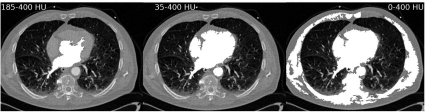
Three segmentation efforts of the contrast-filled phase of the heart CT-scan also shown in Figure 6.1. Different levels of minimum and maximum thresholds result in different ROIs to be segmented. The left image (with a threshold range of 185 – 400 HU) shows parts of the atrium, the left ventricle, and the aortic valve. Choosing a wider threshold of 35 – 400 HU also segments the parenchyma of the heart, and a small bridge also causes segmentation of the descending part of the aorta. When using a window of 0 – 400 HU, too many image elements are connected to the original seed, and large parts of muscle tissue and the skeleton are segmented as well. Image data courtesy of the Dept. of Radiology, Medical University Vienna.
Another problem with region growing in real life is the fact that anatomical regions do usually not show a sharp and continuous border to surrounding tissue. As the threshold window width grows, small “whiskers” usually appear in the segmented mask, which finally lead to a flooding of the whole image. These small structures are usually referred to as bridges; the straightforward way to deal with those is to manually introduce borderlines which must not be crossed by the region growing algorithm. In Example 6.8.3, you can experiment with implementing such a borderline. In real life, these bridges appear pretty often and require additional manual interaction, which is certainly not desirable. The middle and right part of Figure 6.4 show several bridges.
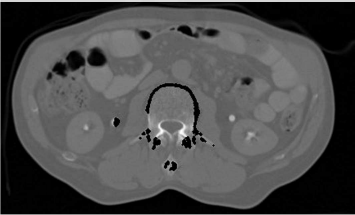
Having said all that, the most important problem is given by the fact that in medical imaging we often deal with 3D images, which are given as series of slices. While it is simple to apply global operations such as intensity transforms and thresholding, region growing in its raw form is pretty unsuitable for segmenting 3D volumes. In addition to adequate parameters for selecting the neighbors that belong to the structure to be segmented, we also need a method to propagate the seed through the volume, which is usually segmented slice-wise. If one naively transfers the seed to the next slice, the algorithm is bound to fail. The reason is the fact that structures which are connected in 3D may appear as separate structures in a single slice. A classical example is the aorta. If one looks at a contrast-enhanced CT scan of the heart like in Figure 6.4 it is evident that the aortic valve, the atrium and parts of the left ventricle are well saturated with contrast agent. The aorta, which leaves the heart in a caudal direction and makes a 180° turn (the aortic arch) to go down the spine, may appear as two circular structures on a single slice. Figure 6.5 illustrates this problem. Apparently it can be a difficult task to segment this structure using a slice-wise 2D region growing algorithm without additional knowledge of 3D anatomy. This 3D knowledge can be introduced by other methods such as statistical shape models or by level set methods, which will be introduced later on, but by itself, 2D-region growing cannot cope with such a problem.
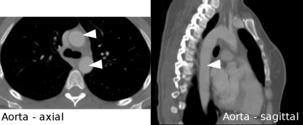
An illustration of typical problems encountered when dealing with 3D segmentation problems. The aorta in these CT images (indicated by white arrows) appears as a single structure in the right slice, which is reformatted in a sagittal orientation, whereas it shows up as two circles in the left axial slice. Image data courtesy of the Dept. of Radiology, Medical University Vienna.
6.5 More Sophisticated Segmentation Methods
As pointed out before, segmentation of 3D structures can become intrinsically more delicate. In the following practical lessons, you will find two examples in Section 6.8.4, which give an illustration. Here, we demonstrate the effects of intelligent seed propagation in 3D. In general, all segmentation methods try somehow to define a ROI by following contours; they are, indeed, always based on propagating some kind of reference position towards a significant structure. In general, it might therefore be a good idea to apply some of the intensity transforms already encountered in Chapter 4. Furthermore, it might also prove useful to emphasize ridge lines that might correlate with anatomical structures using some of the methods from Chapter 5. The general problem of segmentation, however, stays the same – there is no simple solution to tell whether the intensities in an image give a good measure if an image element belongs to an anatomic structure or not. Therefore, the number of sophisticated algorithms published is considerable and goes beyond the scope of this book. For the sake of completeness, I will nevertheless try to give an outline of the common segmentation approaches.
Snakes or active contours: In general, snake-type algorithms are a special case of deformable models applied to volume data in a slice-wise manner. One may start with a general contour model, which adopts itself to a given contour by optimizing some sort of energy function. You may recall from Chapter 3 that an image is a mathematical function, which maps gray values ρ to pixel or voxel coordinates. ρ can be considered the height of a landscape – the valleys are, for instance, black, and the mountaintops are white. We know from basic physics that we can store potential energy when bringing a massive body to a mountaintop. If the points of our contour model are considered massive bodies, we may be able to find a contour by maximizing the potential energy. Example 6.8.5 gives a very simple illustration of this concept. Again, things are not as simple as they may sound – one has to define further boundary conditions. One of them may be that the adjacent points should stay close to each other, or more mathematically speaking, that the contour is steady and smooth. Or we may assume that the gain in potential energy of our mass points is diminished if they have to travel a very long way – in other words, it may be better to position your contour point on the nearest local peak of the ridge, rather than looking for the highest of all peaks. Finally, snakes are implicitly two dimensional. This is somewhat straightforward in medical imaging, where volume data are usually presented as slices. Still this is not very useful for many cases. Remember the example of the aorta in Section 6.4. A single anatomic entity such as the aorta may appear divided when looking at some of the slices. Therefore, the simple 2D way of looking at volumes is very often not optimal for segmentation tasks.
Live wire segmentation: A somewhat similar algorithm is the live wire algorithm, which takes a few edge points and fills the gaps to a contour; the merit function to be optimized for the image mainly operates on a gradient image, which can be derived by using edge detection methods such as those presented in Chapter 5.
Watershed transform: Another segmentation method for contours or contours derived from differentiated images is the watershed transform. Again, the contour of an image is considered a ridge line of a mountain range. When attaching buoys on each point of the ridge with a long rope, all you need is to wait for a diluvian and the line of buoys gives you the watershed transform of the mountain range. In other words, the valleys in the image are flooded, and while the water masses merge, they somewhat remember that they rose from different parts of the image.
Shape models: A technique to utilize a-priori knowledge of the organ to be segmented is the use of statistical shape models. Here, a gross average model of the organ to be segmented is generated from a large population of segmented 3D regions. Certain basis vectors for these shapes are computed by means of a principal component analysis (PCA). More details on the PCA and those basis vectors can be found in Chapter 7. In general, these shape models can be represented by a number of methods. The most simple way is to use the nodes of a surface mesh. Once a shape model is generated, it can be deformed by a linear combination of basis vectors. Intensity information, however, remains the main objective; the algorithm that selects the coefficients for the linear combination still relies on thresholding, region growing, or similar basic algorithms. However, by adopting the shape model, one also gets additional boundaries which mimic the organ to be segmented. The major advantage of shape-model type algorithms lies in the fact that it is 3D by nature and is not constrained by proceeding through slices, and that it takes more information than just the gray values of the image into account. Its disadvantage lies in the fact that the generation of the model requires a large number of representative samples, which all have to be segmented from clinical data. Furthermore, the use of a model constrains the algorithm’s flexibility. One may generate, for instance a brain model. If this model is applied to a patient who underwent a neurosurgical procedure where part of the brain was removed, the algorithm is bound to fail. Unfortunately, we often encounter sick patients.
Level set segmentation: This is another method that utilizes some knowledge from beyond the intensity domain. Segmentation of a 2D image using level sets takes place by intersecting the 2D image with a surface model from 3D; in an iterative process, the higher-dimensional surface model given by a partial differential equation (PDE) may change its appearance until the intersection of the 3D surface with the 2D image yields the desired contours. It is of course also possible to intersect a 4D surface with a 3D volume, therefore the method is also an intrinsic 3D segmentation method. The adaptation of the higher-dimensional surface takes place by means of a so-called speed function, which is of course again coupled to image intensities. Active contours do offer the possibility to define the speed function.1
6.5.1 ITK SNAP – a powerful implementation of a segmentation algorithm at work
A beautiful implementation of a more sophisticated segmentation algorithm can be found if one searches for a program called ITK SNAP2. Figs. 6.6, 6.7 and 6.8 show the workflow of a typical segmentation progress, here again of a heart.
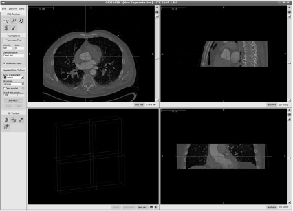
A screenshot of ITKSnap in its initial stage. Again, the heart CT scan already familiar from Figure 6.4 is used. The user can place a cross hair at an axial, sagittal and coronal slice; this is the 3D seed for the algorithm. Here, it is placed at the approximate location of the aortic valve. Image data courtesy of the Dept. of Radiology, Medical University Vienna.
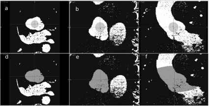
ITKSnap in progress. a, b and c show the initial bubble in the thresholded volume in axial, sagittal and coronal view. This is the zero level of the level set method. An appropriate global intensity threshold was also already applied to the image. As the algorithm iterates, it shows a constant growth in three dimensions, which reflects the change in the shape of the higher-dimensional manifold. This shape is bound by the borders indicated by the threshold. Note that the bubble does not penetrate every single gap in the pre-segmented image – it has a certain surface tension that keeps it from limitless growth. d, e and f show an intermediate stage of the segmentation process. Image data courtesy of the Dept. of Radiology, Medical University Vienna.
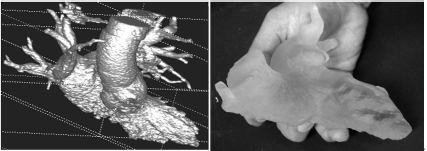
The result of the segmentation using ITKSnap after rendering (image on the left). The contrast agent’s distribution mirrors the disease of the patient; he suffers from severe heart insufficiency, which causes little transport of the arterial blood and the contrast agent. Therefore, venous structures are also partially segmented. This 3D surface model can be “cleaned up” and smoothed using morphological operations, and transformed to a surface model – these techniques will be introduced in a later chapter. Once a triangulated surface model is available, the model can be printed using a 3D stereo lithographic printer. This tangible 3D model is shown in the photograph on the right.
In short, ITK-SNAP utilizes an active contour model, which evolves based on the level set method. Intensity information from the image, together with an initial thresholding step are used for the definition of a primary model (called a bubble in ITK-SNAP) which evolves iteratively. The evolution is defined by a partial differential equation that also defines the shape of the higher-dimensional surface for the level set method. For the simple MATLAB-scripts used throughout this introductory course, the method is already too complex for a sample implementation. However, the reader is encouraged to download ITK-SNAP and to experiment with its capabilities.
6.6 Morphological Operations
After a gross overview of the basic principles of segmentation, we also have to introduce a class of operations that are referred to as morphological operations. Once a model was segmented more or less successfully, one may encounter some residual debris, which may stem from intensity bridges – which is quite often the case when using region growing methods. Another source of stray image elements that are not connected to the actual segmented ROI may be image noise; when segmenting image data from nuclear medicine, this is actually pretty common since the main ROI can usually be segmented by thresholding.
A method to get rid of such segmented image elements that are either loosely connected or completely unconnected is a process called erosion. Erosion is the digital equivalent to sandblasting. When one wishes to clean a rusty piece of machinery, the method to clean such a piece of metal is to use an abrasive that is blown with high pressure onto the workpiece. The abrasive removes the surface layer of loose material and produces a ground surface. But as long as one does not use too much pressure or blasts onto one position for hours, the general structure of the workpiece is maintained. Erosion does the same thing to our segmented model. A kernel of defined shape wanders through the image; whenever the center of the kernel encounters an image element that is not zero (remember that the segmented model is usually binary), it checks whether its neighbors are non-zero as well; if the kernel is not completely contained within the segmented shape, the pixel at the center is removed. Mathematically speaking, the result of the erosion operation is the intersection of the original shape and the kernel. One may also remember the convolution operation introduced in Chapter 5, where a kernel is – figuratively spoken – intermixed with the image. The erosion operation is something similar, although it is non-linear by nature.
The opposite of erosion is dilation. Here, the union of the kernel and the shape is formed. If the center of the kernel lies within the segmented structure, it appends its neighbors to the shape. As a mechanical example, dilation can be compared to the coating of the shape with some sort of filler. Small defects in the shape, which might also stem from noise, can be closed by such an operation. In order to illustrate this operation, a rectangle with a small additional structure was drawn using the GIMP, and both erosion and dilation were applied. The result can be found in Figure 6.9.

The effect of erosion and dilation using GIMP on a very simple shape (left image). After erosion, the rectangle is somewhat slimmer, and the internal additional structure is removed. Dilation causes the opposite effect; the internal structure was fused with the rectangle, and the whole rectangle got wider. Example 6.8.6 allows you to play with this image of 20×20 pixels. The shaping element is an eight-connected kernel of 3×3 pixel size.
The two operations can also be used together; if one applies an erosion followed by a dilation operation, the process is called opening; single image elements are removed by the erosion, and therefore cannot be dilated afterwards. Non-zero image elements enclosed by the segmented structure are widened and therefore are more likely not to be filled completely by the dilation process. The opposite operation – dilation followed by erosion – is called closing.
Here, small black image elements within the segmented region are filled before the erosion process can open them up again. The advantage of both combined operations lies in the fact that they leave the surface and the shape of the segmented region somewhat invariant. Erosion by itself results in a thinner shape with less area than the original segmented shape. The dilation process compensates for this.
Given the fact that the generalization of erosion and dilation to 3D is pretty straightforward, it is evident that both operations can be extremely helpful when it comes to simplification and smoothing of segmented 3D models. Figure 6.8 gives a good illustration. The segmented 3D model of the left ventricle, the atrium, and the aorta was smoothed using an erosion process, which removed both loose residual 3D voxels and fine filaments connected to the pulmonary veins. In the fused deposition modelling process that generated the model shown in the left part of Figure 6.8, these fine structures would have caused considerable additional cost since the process deposits a fine powder in layers, which is cured by ultraviolet light. Each single stray voxel therefore requires a considerable deposit of so-called support material, which is necessary to keep the (completely useless) structure in position during the generation of the model.
6.7 Evaluation of Segmentation Results
Finally, we introduce two measures on the evaluation of segmentation results. If a model is segmented by an algorithm, it should be possible to compare this result to a gold standard segmentation. The first measure to evaluate the match of two contours is the Hausdorff-distance of two graphs. The Hausdorff-distance gives the maximum distance between to surfaces or contours. As a matter of fact, it is easier to program a Hausdorff-distance than to explain it. Let’s consider two sets of contour points, S1 and S2. Each point si of contour S1 has a set of distances {di} to all other points of contour S2. If we select the smallest of these distances in this set {di}S1→S2 (this is the infimum) and proceed to the next point of S1, we end up with a set of minimal distances for each point in S1 to all other points in S2. The maximum of this set is called the supremum. It is clear that if we perform the same operation for all points in S2, the result can be different because the smallest distance of a point in S2 to S1 can be completely different from all the distances in {di}S1→S2. Figure 6.11 illustrates this. The Hausdorff-distance is defined as
.
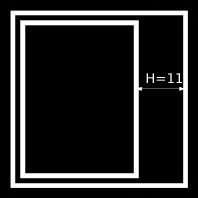
Two very simple shapes; the original image is used in Example 6.8.8.1 and is 40 × 40 pixel large. The Hausdorff distance is 11 pixels and is drawn into the image. There are of course larger distances from points on the inner rectangle to the outer square. But the one shown here is the largest of the possible shortest distances for points on the two shapes.
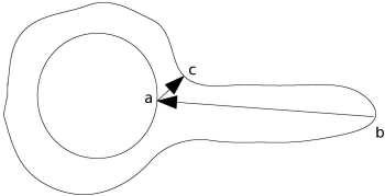
An illustration of the asymmetric nature of the Hausdorff distance. The minimum distance from point a to the outer shape leads to point c, whereas the shortest distance from point b on the outer shape leads to point a.
Besides being a tool for evaluation, the Hausdorff-distance does of course also allow to construct a segmentation criterion, for instance in an active contour model.
The other measure is a little bit easier to understand; it is the Dice-coefficient, defined by the overlap of two pixel sets A1 and A2. It is given as
|A1 ∩ A2| is the absolute number of intersecting pixels (the pixels that share the same area) and |Ai| is the sum of pixels in each area. Example 6.8.8.1 illustrates both concepts.
6.8 Practical Lessons
6.8.1 Count rate evaluation by ROI selection
ROIExample_6.m implements the evaluation of activity in a given ROI, a common procedure from nuclear medicine. Here, we have a very simple series of images. It is a Petri-dish filled with a radioisotope, placed on a γ-camera. In the folder ROI in the LessonData, you find eight DICOM files alongside with the corresponding JPG images. Figure 6.12 shows a part of two of those images. A typical task in nuclear medicine is the monitoring of clearance rates of a tracer. For this purpose, one usually defines a ROI and measures the intensity as detected by the γ-camera or another modality for nuclear medicine. In this example, the ROI is the whole image since we only see the Petri dish. We therefore have to open the eight images, sum up the intensity in the ROI, and compare the results of this time series.
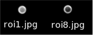
Two out of the eight images used for this example. We see the image of a Petri–dish filled with a radioisotope taken with a γ-camera. The bottom of the dish features a rim; according to the inverse-square law, the rim is brighter than the bottom of the dish, which is slightly elevated over the scintillator. The right image was taken at a later point in time, therefore the intensity in the image is lower. Image data courtesy of the Dept. of Nuclear Medicine, Medical University Vienna.
First, we have to change the working directory to the ROI directory by using the cd ROI command, and we have to find out about the DICOM-header sizes of the eight files in the ROI directory; I have already computed those header sizes. These are stored in a vector called headersize:
1:> cd ROI;
2:> headersize=zeros(8,1);
3:> headersize(1,1)=5710;
4:> headersize(2,1)=5712;
5:> headersize(3,1)=5682;
6:> headersize(4,1)=5696;
7:> headersize(5,1)=5702;
8:> headersize(6,1)=5700;
9:> headersize(7,1)=5704;
10:> headersize(8,1)=5698;
Next, we will allocate the matrix for the 256 × 256 image of 16 bit depth, and the vector for the cumulative image intensities. A text file storing the data will also be created:
11:> img = zeros(256,256);
12:> intens=double(zeros(8,1));
13:> ifp=fopen(’Intensities.txt’,’w’);
In the next few steps, we will open all eight DICOM files, skip their headers (whose size is stored in the headersize vector), and sum up the pixel intensities of the images. These are stored in a text file and plotted.
14:> for ind=1:8
 15:> message=sprintf(’Reading file #%d
’,ind);
16:> fname=sprintf(’roi%d’,ind);
17:> fp=fopen(fname, ’r’);
18:> fseek(fp,headersize(ind,1),’bof’);
19:> img(:)=fread(fp,(256*256),’short’);
20:> fclose(fp);
21:> intsum = 0;
22:> for j=1:256
23:> for k=1:256
24:> rho = double(img(j,k));
25:> intsum = intsum + rho;
26:> end
27:> end
28:> intens(ind,1)=floor(intsum);
 29:> fprintf(ifp,’%d
’,intens(ind,1));
30:> end
31:> fclose(ifp);
32:> plot(intens)
33:> cd ..
All of this you have seen before, and the example so far is trivial. It can even be made more simple if you use the dicomread functionality available in MATLAB’s image processing toolbox. So here is the part that requires some work on your side:
Additional Tasks
Which isotope was used?
Repeat the procedure with roi....jpg images in the ROI folder; the corresponding file ROIExampleWithJPGs_6.m is also in the LessonData-folder. What is the result for the radioisotope, and why is it wrong?
In order to answer the first question, you have to find out about the half-life of the isotope. For this purpose, one has to find out about the time between the images. This can be done by checking the DICOM-header. Tag (0008|0032) gives you the acquisition time as a text string as hour, minute and second. You can write the acquisition times in a spreadsheet and plot the content of the Intensities.txt file with the appropriate time intervals. What you see then is the reduction of cumulative image intensity caused by the decay of the isotope. The recorded image intensity is proportional to the radioactive nuclei available, and their number follows the law of radioactive decay:
N(t) is the number of nuclei at time t, and N(t0) is the number of nuclei when the measurement starts. λ is the so called decay constant. The half-life is given as . As long as the detector of the γ camera takes its measurements in a more or less linear part of its dynamic range (see Figure 4.2), the cumulative image intensity at time t is proportional to N(t). Therefore, half-life can be computed from the data in the Intensities.txt file. As a further hint, I can assure you that the isotope used here is a pretty common one in nuclear medicine.
The second question is a more philosophical one. The answer lies in the fact that medical images are not just pretty pictures. Most common image formats like JPG store grayscale images at 8 bit depth, and this is fine if you don’t want to do anything but to look at them. For analytical use, this compression in intensity space is not permissible since the cumulative intensities are no longer proportional to the measured count rate of the γ-camera, which is by itself proportional to the number of nuclei. Remember - we are dealing with mathematical functions showing the physical properties of tissue, we are not just taking photographs. For the same reason, we have used DICOM images in Example 3.7.5 for the computation of SNR values.
6.8.2 Region definition by global thresholding
Here is a simple one; we try a global threshold on the ABD_CT.jpg image provided with the example. The threshold is set to 150. You should try different thresholds and interpret the image. The script is called Threshold_6.m:
1:> img = imread(’ABD_CT.jpg’);
2:> segimg = zeros(261,435);
3:> thresh = 150;
4:> for i=1:261
5:> for j=1:435
6:> if img(i,j) >= thresh
7:> segimg(i, j)=64;
8:> end
9:> end
10:> end
11:> colormap(gray)
12:> image(segimg)
Additional Tasks
The result of Threshold 6.m is a binary image with pixel intensities of 0 and 64; by using image algebra techniques such as the ones introduced in Section 3.1.1 and Example 3.7.1, it is possible to generate a greyscale image of the segmented ROI. Modify Threshold_6.m accordingly.
6.8.3 Region growing
First, we will implement region growing using a very simple 2D image, which is shown before and after segmentation by region growing in Figure 6.13. This is, again, not a very clinical image; however, it is usually a good idea to test algorithms on very simple images before proceeding to the more complex material encountered in real life.

The left image is the original phantom image, which will be used for our example in the first place. After choosing a seed within the head of this little character and an appropriate threshold range, applying a region growing algorithm using four-connected neighbors results in the right image.
So here we go with a very simple implementation of region growing; the script is found in the LessonData folder, and it is named RegionGrowing_FourConnected_6.m. As usual, we open the image first, and we cast it by force to the data type uint8. A second matrix named seedmask is openend, and an initial seed is placed at the pixel coordinate (130, 210). This seed assumes the value 64 as opposed to the remainder of the matrix. The intensity of the pixel at the location of the seed is retrieved:
1:> img = uint8(imread(’PACMAN_THINKS.jpg’));
2:> seedmask=zeros(261,435);
3:> seedmask(130,210)=64;
4:> seedintensity=img(130,210);
Next, we define a range of possible pixel intensities around the intensity of the seed; here, we define a range of ±10 gray values around the intensity of the seed. If these intensity limits are beyond the image range, they are truncated to the upper and lower bound of the image range. Strictly speaking, this is not necessary since too large a range will not affect the outcome. But it is good manners to take care of things like that:
5:> seedrangemin=seedintensity-10;
6:> if seedrangemin < 0
7:> seedrangemin = 0;
8:> end
9:> seedrangemax=seedintensity+10;
10:> if seedrangemax > 255
11:> seedrangemax = 255;
12:> end
Now, an iterative process is started; we initialize two counter variables, oldseeds and newseeds, which hold the number of seeds during each iteration. After that, we enter a while-loop, which terminates when no new seeds are found in the next iteration – the operator ~=, which is “not equal” in MATLAB, is introduced here. In each iteration, the newseeds found in the previous run become the oldseeds of the current run. Next, we inspect every pixel of the image seedmask containing the seeds; only the pixels on the very edge of the image are not taken into account since this simplifies life when looking for neighboring pixels (otherwise we would need a special check whether we are still inside the image while looking for neighbors). If a seed is encountered, the algorithm looks whether the image intensity intens of its four-connected neighbors is within the intensity range; if this is the case, these neighbors also become seeds. The while loop terminates if the number of seeds becomes constant. Finally, the segmented area, stored in seedmask is displayed. The results should resemble the right image in Figure 6.13. However, the image is a 1 bit image, which simplifies the segmentation task considerably.
13:> oldseeds = 1;
14:> newseeds = 0;
15:> while newseeds ~= oldseeds
16:> oldseeds = newseeds;
17:> newseeds = 0;
18:> for i = 2:260
19:> for j = 2:434
20:> if seedmask(i,j) > 0
21:> intens=img((i-1),j);
22:> if (intens >= seedrangemin) &
(intens <= seedrangemax)
23:> newseeds = newseeds + 1;
24:> seedmask((i-1),j) = 64;
25:> end
26:> intens=img((i+1),j);
27:> if (intens >= seedrangemin) &
(intens <= seedrangemax)
28:> newseeds = newseeds + 1;
29:> seedmask((i+1),j) = 64;
30:> end
31:> intens=img(i,(j-1));
32:> if (intens >= seedrangemin) &
(intens <= seedrangemax)
33:> newseeds = newseeds + 1;
34:> seedmask(i,(j-1)) = 64;
35:> end
36:> intens=img(i,(j+1));
37:> if (intens >= seedrangemin) &
(intens <= seedrangemax)
38:> newseeds = newseeds + 1;
39:> seedmask(i,(j+1)) = 64;
40:> end
41:> end
42:> end
43:> end
44:> end;
45:> colormap(gray)
46:> image(seedmask)
Additional Tasks
Another image, PACMAN_THINKS_WITH_A_BRIDGE.jpg, features an artifact. A thin line connects the head of the character with another structure. If you try to segment this image, you will end up with a larger segmented image, containing unwanted areas. You can suppress this by adding an additional border, which can, for instance, be a straight line from pixel coordinates (110,240) to (110,270). In the algorithm, this line should represent a taboo, where no new seeds are accepted. Implement such a border in the RegionGrowing_FourConnected_6.m script so that the original image as in Figure 6.13 is segmented again.
Try to use the algorithm on the ABD_CT.jpg image provided, and segment the vertebral body from the image. The seed can remain on the same location, but you should experiment with the intensity range. Initially, the result is found in Figure 6.14. It may also be useful to manipulate overall image contrast, for instance by applying the algorithms presented in Example 4.5.4. Figure 6.15 shows two more segmentation efforts using region growing that were made using the AnalyzeAVW software; it is evident that the seed location and the intensity window obviously play a crucial role.
The result when using the RegionGrowing_FourConnected_6.m script on the ABD_CT.jpg image. The vertebral body is not fully segmented. Changing the image intensities and the intensity range for the segmentation algorithm may improve the result. However, this segmentation can be directly compared to Figure 6.3. Image data courtesy of the Dept. of Radiology, Medical University Vienna.

Two more segmentations of the vertebral body from the ABD_CT.jpg image. These results were achieved using the Analyze AVW software. As we can see, both seeds are located within the vertebral body; despite the fact that the range for finding connected pixels was adopted, the result varies significantly. As a conclusion, we see that the region growing algorithm is highly dependent on internal parameters. Image data courtesy of the Dept. of Radiology, Medical University Vienna.
6.8.4 Region growing in 3D
In this example, we will show some principles of 3D segmentation. For this purpose, we will again design a simple theoretical phantom. The volume consists of a 3D matrix, where a tubular structure proceeds from slice # 1 to slice # 80. Figure 6.16 shows some of these slices.
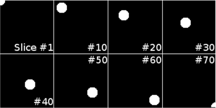
Some of the slices in the simple tube phantom volume generated by the RegionGrowing_WanderingStaticSeed_6.m script. The tube starts at the bottom of the volume in the upper left corner and proceeds along the 3D diagonal of the volume to the lower right corner in the last slice.
So here is the variation of the RegionGrowing_FourConnected_6.m script that operates in 3D. First, a volume named vol with 100 × 100 × 70 voxels is generated. In the following for ... loop, each slice – the z-component of the 3D matrix vol – is visited, and a circle of 19 pixels diameter is drawn. The center of the circle follows the 3D diagonal of the data cube. The if ... statements make sure that only the pixels within a circular shape are drawn into the slices, and that the circles remain within the boundaries of the slices. The script is called RegionGrowing_WanderingStaticSeed_6.m.
1:> vol = zeros(100,100,70);
2:> for i=1:70
3:> sl=sqrt(2*i*i);
4:> for x=-9:9
5:> for y=-9:9
6:> if (x*x+y*y < 100)
7:> sx=floor(sl+x);
8:> sy=floor(sl+y);
9:> if (sx > 0) & (sx < 100)
10:> if (sy > 0) & (sy < 100)
11:> vol(sx,sy,i)=255;
12:> end
13:> end
14:> end
15:> end
16:> end
17:> end
In the next part of the script, we proceed through the volume slice by slice again. For this purpose, again a for ... loop is used, and the slices are copied from the vol datacube to a 2D slice image img.
18:> for slice=1:70
19:> img = zeros(100,100);
20:> for i=1:100
21:> for j=1:100
22:> img(i,j)=vol(i,j,slice);
23:> end
24:> end
What follows is mostly a copy of code from the already well-known RegionGrowing_FourConnected_6.m script. The only difference is the location of the seed, which is given at a static position x = (2,2, # of slice)T; its intensity is also fixed to ρ = 255, and all four connected neighbors within an intensity range of ρ ∈ {245 ... 255} are segmented.
25:> seedmask=zeros(100,100);
26:> seedmask(2,2)=255;
27:> seedintensity=255;
28:> seedrangemin=seedintensity-10;
29:> if seedrangemin < 0
30:> seedrangemin = 0;
31:> end
32:> seedrangemax=seedintensity+10;
33:> if seedrangemax > 255
34:> seedrangemax = 255;
35:> end
36:> oldseeds = 1;
37:> newseeds = 0;
38:> while oldseeds ~= newseeds
39:> oldseeds = newseeds;
40:> newseeds = 0;
41:> for i = 2:99
42:> for j = 2:99
43:> if seedmask(i,j) > 0
44:> intens=img((i-1),j);
45:> if (intens >= seedrangemin) &
(intens <= seedrangemax)
46:> newseeds = newseeds + 1;
47:> seedmask((i-1),j) = 255;
48:> end
49:> intens=img((i+1),j);
50:> if (intens >= seedrangemin) &
(intens <= seedrangemax)
51:> newseeds = newseeds + 1;
52:> seedmask((i+1),j) = 64;
53:> end
54:> intens=img(i,(j-1));
55:> if (intens >= seedrangemin) &
(intens <= seedrangemax)
56:> newseeds = newseeds + 1;
57:> seedmask(i,(j-1)) = 64;
58:> end
59:> intens=img(i,(j+1));
60:> if (intens >= seedrangemin) &
(intens <= seedrangemax)
61:> newseeds = newseeds + 1;
62:> seedmask(i,(j+1)) = 64;
63:> end
64:> end
65:> end
66:> end
67:> end
After each slice, the result is shown; after a few iterations, nothing but the seed itself remains in the image. At that point in time, you may terminate the script by pressing Ctrl-C. The Press RETURN to proceed ... statement halts the script in a very old fashioned way.
68:> colormap(gray)
69:> image(seedmask)
70:> foo=input(’Press RETURN to proceed ...’);
71:> end
Additional Tasks Since it is obvious that this naive approach does not work in 3D, you should find a method to change the seed position in such a manner that the whole tube is being segmented. Two methods of migrating the seed appear straightforward.
Instead of just pushing the seed up one slice, you can compute the centroid of your segmented ROI according to Equation 6.1, and use this position as your new seed after propagating it to the next slice. As long as the tube does not get too thin (which is not the case here), you should be able to succeed.
You may also push your seed to the next slice and initiate a search within a finite radius which looks for pixels in the desired intensity range. As soon as a pixel is found, it becomes the new seed. If no pixel is found, you may terminate the script.
In order to make the whole thing a little bit less tedious to watch, you may add an if clause at the end of the script which only shows every tenth segmented image:
...:> if mod((slice-1),10) == 0
...:> image(seedmask)
...:> foo=input(’Press RETURN to proceed ...’);
...:> end
...:> end
In this example, we have introduced an important principle of advanced segmentation algorithm, which may be described as adaptive – the seed (or, in more complex algorithms, the boundary) of the segmented ROI adopts itself to a new situation using prior knowledge.
6.8.5 A very simple snake-type example
SimpleSnakeSeeds_6.m is another example where we try to segment the vertebral body from the ABD_CT.jpg image. Spoken in a highly simplified manner, snakes are graphs that adopt themselves to border lines of strongly varying intensity in an image. In our example, we will initiate such a graph by drawing a circle around the vertebral body. Figure 6.17 shows the initial phase and the result of the SimpleSnakeSeeds_6.m script. The seeds search for the brightest pixel in a nearby area, and we hope that these correspond to the structure we want to segment.

The initialization phase and the outcome of the SimpleSnakeSeeds_6.m script. First, seeds are defined around the vertebral body by placing them on a circle of 50 pixels radius. Then, the brightest pixel within a range of 20 pixels is determined. The seed migrates to that position. As we can see, the result shows some outliers where the seeds migrated to the contrast-filled leg arteries. Also, the subtle structure of the dorsal part of the vertebral body is not covered very well. Image data courtesy of the Dept. of Radiology, Medical University Vienna.
So here is the code of the SimpleSnakeSeeds_6.m:
1:> img = imread(’ABD_CT.jpg’);
2:> img=transpose(img) ;
3:> edgepoints=zeros(400,2);
4:> numberOfValidEdgepoints=0;
5:> for x=-50:50
6:> for y= -50:50
7:> if ((x*x+y*y) > 2401) & ((x*x+y*y) < 2601)
8:> numberOfValidEdgepoints =
numberOfValidEdgepoints+1;
9:> edgepoints(numberOfValidEdgepoints,1) = 210 + x;
10:> edgepoints(numberOfValidEdgepoints,2) = 145 + y;
11:> end
12:> end
13:> end
So far, we have read the well-known ABD_CT.jpg image, and switched the rows and columns of the resulting matrix. A 400 × 2 matrix edgepoints is allocated, which should hold a number of seeds. None of these edgepoints is allocated so far, therefore the counter numberOfValidEdgepoints is set to zero. Next, we define the coordinates of a circle of radius 50 around pixel using the well known parametric representation of a circle x2 + y2 = r2 where x and y are the Cartesian coordinates of the diameter of the circle, and r is its radius. In order to avoid round-off errors from our discrete coordinates, every coordinate where is within the range of {49...51} is accepted. The result can be found in the left half of Figure 6.17. Next, we will instantiate a search for the brightest pixel in a neighborhood of radius searchradius = 20 pixels.
14:> searchrad=20;
15:> for ei=1:numberOfValidEdgepoints
16:> ximax = edgepoints(ei,1);
17:> yimax = edgepoints(ei,2);
18:> imax=img(ximax,yimax);
19:> for x=-searchrad:searchrad
20:> for y=-searchrad:searchrad
21:> if ((x*x+y*y) < (searchrad*searchrad))
22:> xs=edgepoints(ei,1)+x;
23:> ys=edgepoints(ei,2)+y;
24:> if img(xs,ys) > imax;
25:> imax=img(xs,ys);
26:> ximax=xs;
27:> yimax=ys;
28:> end
29:> end
30:> end
31:> end
32:> edgepoints(ei,1)=ximax;
33:> edgepoints(ei,2)=yimax;
34:> end
All pixels within the edgepoints-matrix are visited, and using the already known parametric representation of a circle, the brightest pixel within searchradius is sought after. We also remember the coordinates of this brightest pixel using the variables ximax and yimax. After the search, the coordinates of an edgepoint are reset to the coordinates of this brightest pixel. All we have to do now is mark this position of the new edgepoints by drawing a small black cross at this position, and furthermore, the result is displayed using image. The result can also be found in the right part of Figure 6.17.
35:> for ei=1:numberOfValidEdgepoints
36:> img(edgepoints(ei,1)+1,edgepoints(ei,2)) = 0;
37:> img(edgepoints(ei,1),edgepoints(ei,2)) = 0;
38:> img(edgepoints(ei,1)-1,edgepoints(ei,2)) = 0;
39:> img(edgepoints(ei,1),edgepoints(ei,2)+1) = 0;
40:> img(edgepoints(ei,1),edgepoints(ei,2)-1) = 0;
41:> end
42:> img=transpose(img);
43:> maximg=double(max(max(img)))/64.0;
44:> img=img/maximg;
45:> colormap(gray)
46:> image(img)
The result is, admittedly, not very convincing. A few edgepoints migrated towards intense structures such as the femoral artery, and many converged to the same location, resulting in a very sparse outline. However, some of them did somehow find the cortex of the vertebral body.
The problem here lies in the fact that the energy of the single edgepoint – remember the introduction of the snake-algorithm in Section 6.5 – is defined in a very trivial way. We simply search for the highest peak within the search radius searchrad. A more intelligent version of our algorithm should consist of additional boundary conditions that define the energetic optimum. For instance, we can add a term that diminishes the potential energy if we try to place our edgepoint at a position that is already occupied by another edgepoint. The easiest way to achieve this is to set the intensity of a peak in the ridge of intensities to zero. A subsequent edgepoint will therefore find this position to be ineligible for an edge point, and will search for another maximum within searchrad. A modified script, BetterSnakeSeeds_6.m, does exactly this. The assignment
...:> edgepoints(ei,1)=ximax;
...:> edgepoints(ei,2)=yimax;
from SimpleSnakeSeeds_6.mis augmented by another assignment in BetterSnakeSeeds.m:
...:> edgepoints(ei,1)=ximax;
...:> edgepoints(ei,2)=yimax;
...:> img(ximax,yimax)=0;
The result is found in Figure 6.18. Compared to Figure 6.17, we see an improvement, although we still face the problems that some of our contour points still migrate to other structures of high intensity.
The result of the BetterSnakeSeeds_6.m script. Here, seeds cannot select the same position as an intensity maximum. Still, some seeds wander off to other structures since we have not yet introduced a criterion of contour smoothness. Image data courtesy of the Dept. of Radiology, Medical University Vienna.
Additional Tasks
In this oversimplified example, we were at least able to define parts of the cortex of the vertebral body. Still we are far from a satisfying result. Therefore, it would be interesting to take a few more measures. The one measure that might really help in this endeavor, however, would be a smoothness constraint on the contour; in a very simple manner, this can be introduced by taking care that neighboring contour points stay close together when migrating from the initial shape to the most intense pixel available. A simple way to achieve this in BetterSnakeSeeds_6.m is to move each point to the position of its predecessor before starting a search for a maximum pixel. The only problem here is a rather technical one. We have to take care that all the starting positions are sorted, so that two neighboring edgepoints are also indexed next to each other. This was done in a third script BetterSnakeSeedsCon-strained_6.m. The result of BetterSnakeSeedsConstrained_6.m can be found in Figure 6.19. Compared to the earlier efforts from Figs. 6.17 and 6.18, the result is more encouraging – at least all the edgepoints finally migrated to the vertebral body, although the contour is still not well defined. Your task with this script is to inspect the code from BetterSnakeSeedsConstrained.m and find out what actually happens. Sorting the edgepoints is, by the way, achieved with the nasty old trick from Example 3.7.5. Why is this sorting necessary? Finally, you might also try to use some of the windowing and edge-enhancement operations from Chapters 4 and 5 to further improve the result.

The result of the BetterSnakeSeedsConstrained_6.m script. By taking a few additional measures, smoothness of the contour was introduced in such a manner that each of the edgepoints searches for a maximum intensity in the immediate vicinity of its predecessor, who has already found a maximum. By this, it is made sure that the single edgepoints stay together. On the other hand, a full contouring of the cortex of the vertebral body has not been achieved. Image data courtesy of the Dept. of Radiology, Medical University Vienna.
We stop further efforts to refine the result of our contour-based segmentation algorithm, which is, in its simplicity, more a mixture of ideas from various segmentation methods. One possibility would be, for instance, adding the Hausdorff-distance as a further constraint. By subsequently adding constraints, we were able to refine the result – first, we were just pushing contour points towards the maximum pixel intensity ρ available. Second, we added the constraint that contour points must not occupy the same position, therefore the contour cannot contract to a single point. Finally, we told the contour points to stay close to each other. Figure 6.20 illustrates our approach. If we would continue our efforts, we might even be able to get a full segmentation of the vertebral body, but the effort to achieve this would make a rather extensive script necessary. Furthermore, we could also let our edgepoints propagate similar to the seed in Example 6.8.4 in order to get a three dimensional segmentation. In the case of region growing, we learned that the algorithm is highly dependent on internal parameters such as the intensity range defining the region, and initial seed location. We conclude from this example that this dependence on a proper choice of parameters also holds true for other algorithms such as contour models.
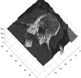
A surface plot of the vertebral body from ABD_CT.jpg illustrates our measures taken in the snake-type segmentation example. The image was inverted, and the contour of the vertebral body to be segmented now appears as a deep ridge in this plot. In the first example, we arranged a ring of marbles around the cortex of the vertebral body, and most of them fell into this groove, but they were infinitely small – therefore, several marbles could take the same place. In the next refinement, only one marble could take a position at the bottom of the groove. In the third step, we made magnetic marbles. The contour points stick to each other, and therefore they take positions at the bottom of this surface next to each other. In Example 6.8.8.2, we will deepen the groove using filtering techniques.
6.8.6 Erosion and dilation
MorphologicalOps_6.m is a script that implements erosion on the very simple shape from Figure 6.9. Let’s take a look at it:
1:> img = imread(’MorphologicalSquare.jpg’);
2:> modimg = zeros(20,20);
So far, nothing new. We have opened an image, and allocated the memory for another image of the same size, which will contain the result of the operation. Next, we will visit every pixel besides those on the very edge of the image; if we encounter a non-black pixel, we will copy this pixel to the new image modimg. If we see that there is a neighbor that is zero, this pixel is deleted. The kernel hides in the if statement – the operator || is a logical OR, by the way.
3:> for i=2:19
4:> for j=2:19
5:> if img(i,j) > 0
6:> modimg(i,j)=1;
7:> if (img(i-1,j) == 0) || (img(i+1,j) == 0) ||
(img(i,j-1) == 0) || (img(i,j+1) == 0)
8:> modimg(i,j) = 0;
9:> end
10:> end
11:> end
12:> end
13:> colormap(gray)
14:> image(64*modimg)
Finally, the image is displayed. Figure 6.21 shows the result.

A shape, generated by erosion in MorphologicalOps_6.m from the shape MorphologicalSquare.jpg, which can be found in the LessonData folder and Figure 6.9. Denote the difference in this shape and the middle image in Figure 6.9, which was generated by using the erosion operator in the GIMP.
Additional Tasks
Modify the erosion kernel in such a manner that MorphologicalOps_6.m produces the same eroded shape as GIMP in Figure 6.9.
Modify MorphologicalOps_6.m in such manner that it performs a dilation, an opening, and a closing operation.
Threshold ABD_CT.jpg and perform some morphological operations on the result.
6.8.7 Hausdorff-distances and Dice-coefficients
Hausdorff_6.m implements a Hausdorff-distance on Figure 6.10. We have two images Hausdorff1.jpg and Hausdorff2.jpg, which can be combined to Figure 6.10. Let’s take a look at the script; we read the two images, and we allocate a vector for the two Hausdorff-distances as well as a vector d which holds all possible distances for a point. ind is a counter variable:
1:> imgOuter = imread(’Hausdorff1.jpg’);
2:> imgInner = imread(’Hausdorff2.jpg’);
3:> dmax=zeros(2,1);
4:> d=zeros(1600,1);
5:> ind=1;
Next, we enter imgInner and if we encounter a non-zero pixel, we start computing its distance dd to all non-zero pixels in imgOuter. If dd is smaller than the smallest distance dist encountered so far, it is declared to be the smallest distance. dist is initialized to the diagonal of the 40 × 40 images, and by this, we compute the infimum of all distances. When all pixels in imgOuter were visited, this infimum of distances is stored in the vector d. If we are done with all pixels in imgInner, we determine the supremum of all distances as the maximum member of d and store it in the vector dmax. The same procedure is repeated with imgInner and imgOuter permuted, but this part of the code is not printed here. The Hausdorff-distance is the maximum of the two values in dmax. In this case, the two Hausdorff-distances are the same due to the geometric shape of the sample.
6:> for i=1:40
7:> for j=1:40
8:> if imgInner(i,j) > 0
9:> dist=57;
10:> for k=1:40
11:> for l=1:40
12:> if imgOuter(k,l) > 0
13:> dd=sqrt((i-k)^2+(j-l)^2);
14:> if dd < dist
15:> dist=dd;
16:> end
17:> end
18:> end
19:> end
20:> d(ind,1) = dist;
21:> ind=ind+1;
22:> end
23:> end
24:> end
25:> dmax(1,1)= max(d);
...
...:> HausdorffDistance=round(max(dmax))
Dice_6.m is comparatively simple. It implements Equation 6.3. The images Dice1.jpg and Dice2.jpg are the same as in the Hausdorff-example, but the contours are filled with white pixels. We read the images and compute the area of intersection as well as the areas of the single segmented areas. The resulting Dice-coefficient is 0.73. In an optimum case, it should be 1.
Additional Tasks
In the LessonData folder, you will find the outline of the two segmentation results from Figure 6.15. These are named RGOutline1.jpg and RGOutline2.jpg. Compute the Hausdorff-distance, and compare the two values in dmax.
6.8.8 Improving segmentation results by filtering
In the LessonData/6_Segmentation, you will find a subfolder named ComplexExamples. It contains examples on improving segmentation outcome by filtering and other operations.
6.8.8.1 Better thresholding
In this example, to be found in the subfolder BrachyExample, we have an x-ray taken during a brachytherapy session for treatment of cervical cancer (Figure 6.22). The patient receives a high local dose from small radioactive pellets inserted in the body through hollow needles. This is a multi-exposure x-ray, where the path of the brachytherapy-pellets (seen as bright spots on the image) is monitored while the pellets are retreated. Our (somewhat academic) task is to segment the positioning aid, that shows up as a cross in the image. In a further step, it would be possible to remove this structure from the image by local image interpolation. The x-ray shows a local gradient from right to left, which is most likely caused by the Heel effect.3 One is encouraged to segment the structure from the image, for instance by using GIMP. The original image, already optimized for optimum gray scale representation by using methods similar to those presented in Chapter 4, can be found as image a in Figure 6.24. Thresholding this eight bit image with varying thresholds using GIMP yielded the following results:

An x-ray image taken during a brachytherapy session. The localization of small radioactive pellets in hollow needles is monitored. Therefore, this image is a multi-exposure taken during the dwell times of the pellets, which are retracted by a flexible wire during the irradiation. Our target here is to segment the cross-shaped positioning aid by thresholding. Image data courtesy of the Dept. of Radiation Oncology, Medical University Vienna.

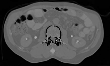
The x-ray image from Figure 6.24 after thresholding. The target structure is the cross-shaped positioning aid. Full segmentation of this image structure is not possible by thresholding. Image data courtesy of the Dept. of Radiation Oncology Medical University Vienna.

a shows the original x-ray, after optimization of image contrast. In order to improve the segmentation of the target structure, several preprocessing steps were carried out. b shows the image after enhancement by unsharp masking. In c, a Sobel filter was applied. This image was thresholded and dilated. The result, which will undergo further processing, can be found in d. Image data courtesy of the Dept. of Radiation Oncology, Medical University Vienna.
In order to improve the segmentation, we can apply various operations which we already know from Chapter 5. First, the image is enhanced using an unsharp masking operation, similar to the operation we have introduced in Example 5.4.4. Next, a Sobel-filter (as it can be found in the examples from Chapter 5) is applied. The result undergoes thresholding and dilation - two operations we know from this chapter. The single preprocessing steps, carried out with GIMP, can be found in Figure 6.24.
Now, we will use some of our own scripts to go further. We could have done all this by ourselves as well, but the result would be the same. Since the cross-shaped structure consists of straight lines, we can apply a Hough-transform. The script from Chapter 5 was changed slightly; it is now named StepOne_Hough_6.m. It produces an image named brachyhough.pgm. In order to compensate for roundoff errors, this image is dilated using a script named StepTwo_DilateHough_6.m, which was derived from the script MorphologicalOps.m described in Example 6.8.6. The result is an image brachydilate.pgm. The third script, StepThree_Threshold_6.m, applies a threshold of 170 to the original image and stores the result as brachythreshold.pgm.
These three scripts are carried out by a fourth script, which is the only script one has to execute if you want to run the sample. It is called BrachyCleanup_6.m. First, it executes the three aforementioned scripts and clears the MATLAB workspace:
1:> StepOne_Hough_6;
2:> StepTwo_DilateHough_6;
3:> StepThree_Threshold_6;
4:> clear;
Next, we read the dilated retransform of the Hough-operation, and we load the threshold image. Both images are scaled to an intensity range of ρ ∈ {0 ... 1}.
5:> dilimg=imread(’brachydilate.pgm’);
6:> dilimg=round(dilimg/255.0);
7:> thimg=imread(’brachythreshold.pgm’);
8:> thimg=round(thimg/255.0);
Now, we allocate memory for a new image, mask, and we perform a pixelwise multiplication of the thresholded image thimg and the dilated Hough-retransform dilimg. The result is a logical AND operation – only if both pixels are non-zero, the pixel in mask is non-zero as well. The results can be found in Figure 6.25. Finally, the result is saved as Cross.pgm and displayed using the image command.

The single steps carried out by the BrachyCleanup_6.m script. Image d from Figure 6.24 undergoes a Hough-transform (a). The result is dilated (b) and undergoes a logical AND operation with the binary result of thresholding at a threshold of 165 (c), which results in the segmented structure d. You are encouraged to compare the result with Figure 6.23, namely illustration b, which was also segmented using the same threshold. Image data courtesy of the Dept. of Radiation Oncology, Medical University Vienna.
9:> mask=zeros(512,512);
10:> mask=thimg.*dilimg*255; ...:>
I admit that this example is a little bit academic, but it illustrates two important aspects of segmentation; first, appropriate preprocessing of the image does help. And second, using a-priori knowledge (in this case the fact that our target structures are straight lines) can be incorporated for better segmentation results. The preprocessing steps shown in Figure 6.24 are also very effective when trying region growing. Figure 6.26 shows the outcome of segmenting the cross structure using the region growing algorithm of AnalyzeAVW.

The effect of region growing on the preprocessed x-ray image shown in Figure 6.24 d. Image data courtesy of the Dept. of Radiation Oncology, Medical University Vienna.
Additional Tasks
Compute the Dice-coefficient and the Hausdorff-distance for the images brachyRegionGrowing.jpg (Figure 6.26) and Cross.jpg, which is the output of the BrachyCleanup_6.m script. Both images can be found in the LessonData folder.
6.8.8.2 Preprocessing and active contours
The same principle of enhancing prominent structures can also be applied to our simple active contour example. The results from Example 6.8.5 were, in the end, already quite good. Still our snake also tends to converge to the inner cortex – this could be solved by modifying our initial shape to a torus – and it tends to neglect the processus transversus. We will try to apply some preprocessing to improve this outcome in the example given in the subfolder ComplexExamples/SnakeWithPreprocessing. Therefore, a few initial steps were applied using GIMP. First, contrast was optimized using a non-linear intensity transform, similar to the Sigmoid-shaped intensity transform from Example 4.5.4. Next, we apply a Sobel-filter; the result undergoes thresholding. The steps are shown in Figure 6.27.

The preprocessing steps carried out using GIMP prior to applying a modified version of the BetterSnakeSeedsConstrained_6.m script. First, non-linear intensity transform is carried out in order to optimize the contrast of the image. Second, a Sobel-filter is applied. The resulting image is thresholded. Image data courtesy of the Dept. of Radiology, Medical University Vienna.
Next, one could apply the BetterSnakeSeedsConstrained_6.m directly to the thresh-olded Sobel-image from Figure 6.27. That is, however, not a brilliant idea since there is absolutely no gradient information in that image. Instead of this simple approach, we invest a little bit more effort in the image to be segmented. A small script named Preprocessing_6.m does all the work; first, it loads the original image ABD_CT.jpg and the image modified using GIMP called ABD_CTSobeledThresh.jpg:
1:> img=imread(’ABD_CT.jpg’);
2:> dimg=imread(’ABD _CTSobeledThresh.jpg’);
Next, it scales dimg to an intensity range ρ ∈ {0 ... 1}, and the intensity range is shifted by one so that black is 1 and white is 2. Next, we avoid problems with the eight bit datatype of our images by scaling the original image img to a range ρ ∈ {0 ... 127}, and we carry out a piecewise multiplication of img and dimg. As a result, the edges of the image are enhanced, and the result is saved as ABD_CT_ENHANCED.jpg.4 The outcome of our operation is a gray scale image with strongly emphasized edges; it can be found in Figure 6.28. The operation we carried out was not very subtle since we have to avoid datatype-related problems for the sake of simplicity, but it serves the purpose.

The result of the Preprocessing_6.m script. It loads the thresholded Sobel image from Figure 6.27, scales the intensities of the original ABD_CT.jpg image appropriately and enhances the edges in the image by a pixelwise binary multiplication. The result is not very beautiful - a more sophisticated operation would require some manipulations in image depth - but the result serves our purpose. Image data courtesy of the Dept. of Radiology, Medical University Vienna.
3:> maxint=max(max(dimg));
4:> dimg=(dimg/maxint)+1;
5:> newimg=zeros(261,435) ;
6:> newimg=0.5*img.*dimg;
7:> imwrite(newimg,’ABD_CT_ENHANCED.j pg’,’JPG’);
The second script we already know - it is a slightly modified version of BetterSna-keSeedsConstrained_6.m named BetterSnakeSeedsConstrainedTwo_6.m. This modified script
carries out Preprocessing_6.m.
operates on the result ABD_CT_ENHANCED.jpg (see Figure 6.28).
has a reduced radius of local search searchrad of 15 instead of 20 pixels.
plots the edgepoints into the original image.
The result can be found in Figure 6.29. Now, at least the processi are also part of the contour, which was not the case in the original script. A further refinement would be possible by changing our initial shape – a circle – to the topologically correct model of a torus. Still, preprocessing by filtering has enhanced the result. In this case, region growing on the differentiated and thresholded image does not yield a satisfying result as it did in Example 6.8.8.1 since the contour cannot be segmented as clearly on the differentiated image.
The result of BetterSnakeSeedsConstrainedTwo_6.m; one may compare the outcome with Figure 6.19. The edge-enhancement operation has led to a better approximation of the vertebral body shape - at least the transverse process is now also part of the contour, which may be refined by using less initial points and a second adaption step which uses interpolated points between those seeds. Image data courtesy of the Dept. of Radiology Medical University Vienna.
6.9 Summary and Further References
Segmentation is certainly one of the more difficult areas in medical image processing. The large body of highly complex and innovative current research work documents this. However, the basic problem is that image intensities map physical properties of tissue, but not the tissue in its entirety. Unfortunately, the more sophisticated the imaging device, the bigger the segmentation problem may become. Segmenting muscle tissue in CT may be cumbersome, but it can be done. An MR image of the same area, which excels in soft tissue contrast, might be even the bigger problem, just because of that very good contrast. However - a large arsenal of segmentation methods exists and the skillful use of these methods should usually solve many problems. Still, manual interaction remains a necessity in many cases. In general, we can categorize the algorithms presented as follows:
Segmentation based on intensity values (thresholding).
Segmentation based on intensity values and one point being part of the ROI (region growing).
Segmentation based on intensity values and a topologically equivalent ROI boundary (snakes and similar algorithms).
Segmentation based on intensity values and a morphologically similar ROI boundary (statisitical shape models).
Sometimes it is also possible to avoid segmentation by using intensity based methods as we will learn in Chapters 9 and 8. In this chapter, only the most basic concepts were introduced: thresholding, region growing, and simple contour based algorithms. An important point also has to be emphasized: segmentation in medical imaging is, in many cases, a 3D problem. A slice-wise approach will not succeed in many cases. Therefore it is necessary to propagate seeds or edge points in an intelligent manner in 3D space.
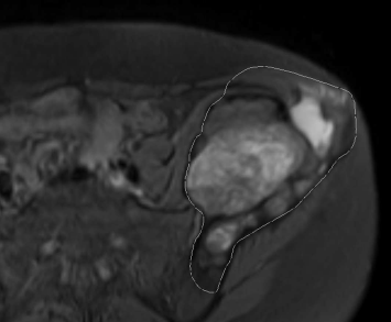
An illustration of the difficulties associated with segmentation. This axial MR slice shows a malignant orthopedic tumor in the hip. The manually drawn border shows the extent of this tumor as drawn by an expert. On image data like this, an automatic segmentation effort will always fail due to the considerable contrast detail of the malignant tissue and the complex and random shape of the lesion. Alternatively, the same lesion shows virtually no detail on other imaging modalities like CT. Image data courtesy of the Dept. of Radiology, Medical University Vienna.
Literature
T. S. Yoo: Insight into Images: Principles and Practice for Segmentation, Registration, and Image Analysis, A. K. Peters, (2004)
J. M. Fitzpatrick, M. Sonka: Handbook of Medical Imaging, Volume 2. Medical Image Processing and Analysis, SPIE Press, (2009)
E. R. Dougherty, R. A. Lotufo: Hands-on Morphological Image Processing, SPIE Press, (2003)
R. Baldock, J. Graham: Image Processing and Analysis: A Practical Approach, Oxford University Press, (2000)
1An introduction to the level set method with MATLAB® can be found in O. Demirkaya, M. H. Asyali, P. K. Sahoo: Image Processing with MATLAB: Applications in Medicine and Biology, CRC Press, 2008.
2A description can be found in PA Yushkevich, J Piven, HC Hazlett, RG Smith, J Ho, JC Gee, G Gerig: User-guided 3D active contour segmentation of anatomical structures: significantly improved efficiency and reliability, Neuroimage 31(3) 1116-1128, (2006)
3The fact that some x-ray photons are trapped inside the anode cause this effect since the photons are generated in a region below the anode surface. Given the fact that the anode is sloped, a gradient in the resulting image is not uncommon.
4If you encounter problems with imwrite in Octave, you may as well save the image as a PGM file.