11
Generalised Linear Models
11.1 Introduction
Like in analysis of variance (ANOVA) or regression analysis a generalised linear model (GLM) describes the relation between a random regressand (response variable) y and a vector xT = (x0, … , xk) of regressor variables influencing it, and is a flexible generalisation of ordinary linear regression allowing for regressands that have error distribution models other than a normal one. The GLM generalises linear regression by writing the linear model to be related to the regressand via a link function of the corresponding exponential family and by allowing the magnitude of the variance of each measurement to be a function of its predicted value.
Possibly the first who introduced a GLM was Rasch (1960). The Rasch model is a psychometric model for analysing categorical data, such as answers to questions on a reading assessment or questionnaire responses, as a function of the trade‐off between (i) the respondent's abilities, attitudes or personality traits and (ii) the item difficulty. For example, we may use it to estimate a student's reading ability, or the extremity of a person's attitude to capital punishment from responses on a questionnaire. In addition to psychometrics and educational research, the Rasch model and its extensions are used in other areas, including the health profession and market research because of their general applicability. The mathematical theory underlying Rasch models is a special case of a GLM. Specifically, in the original Rasch model, the probability of a correct response is modelled as a logistic function of the difference between the person and item parameter – see Section 11.5.
GLMs were formulated by Nelder and Wedderburn (1972) and later by McCullagh and Nelder (1989) as a way of unifying various other statistical models, including linear regression, logistic regression (Rasch model), and Poisson regression. They proposed an iteratively reweighted least squares method for maximum likelihood (ML) estimation of the model parameters. Maximum likelihood estimation remains popular and is the default method in many statistical computing packages. Other approaches, including Bayesian approaches and least squares fits to variance‐stabilised responses, have also been developed. Possibly Nelder and Wedderburn did not know the Rasch model. Later Rasch (1980) extended his approach.
In GLMs, exponential families of distributions play an important role.
11.2 Exponential Families of Distributions
11.3 Generalised Linear Models – An Overview
The term GLM usually refers to conventional linear regression models for a continuous or discrete response variable y given continuous and/or categorical predictors. In this chapter we assume that the distribution of y belongs to the exponential families. A GLM does not assume a linear relationship between the regressand and the regressor, but the relation between the regressor variables (x0, x1, … , xk) and the parameter(s) is described by a link function for which we usually use the natural parameters of the canonical form of the exponential family.
The GLMs are a broad class of models that include linear regression, ANOVA, ANCOVA, Poisson regression, log‐linear models, etc. Table 11.1 provides a summary of GLMs following Agresti (2018, chapter 4) where Mixed means categorical, nominal or ordinal, or continuous.
Table 11.1 Link function, random and systematic components of some GLMs.
| Model | Random component | Link | Systematic component |
| Linear regression | Normal | Identity | Continuous |
| ANOVA | Normal | Identity | Categorical |
| ANCOVA | Normal | Identity | Mixed |
| Log‐linear regression | Gamma | Log | Continuous |
| Logistic regression | Binomial | Logit | Mixed |
| Log‐linear regression | Poisson | Log | Categorical |
| Multinomial response | Multinomial | Generalised logit | Mixed |
In all GLM in this chapter we assume the following:
- All random components refer to the probability distribution of the regressand.
- We have systematic components specifying the regressors (x1, x2, …, xk) in the model or their linear combination in creating the so‐called linear predictor.
- We have a link function specifying the link between random and systematic components.
- y1, y2, …, yn are independently distributed.
- The regressand has a distribution from an exponential family.
- The relationship between regressor and regressand is linear via the link function.
- Homogeneity of variance is not assumed, overdispersion is possible as we can see later.
- Errors are independent but not necessarily normally distributed.
In GLM the deviance means sum of squares and the residual deviance means mean squares. It may happen that after fitting a GLM the residual deviance exceeds the value expected. In such cases we speak about overdispersion.
Sources of this may be:
- The systematic component of the model is wrongly chosen (important regressors have been forgotten or were wrongly included, e.g. linear in place of quadratic).
- There exist outliers in the data.
- The data are not realisations of a random sample.
We demonstrate this for binary data.
Let p be a random variable with E(p) = μ and var(p) = nμ(1 − μ) = σ2. For a realisation p of p we assume that k is B(n; p)‐distributed. Then by the laws of iterated expectation and variance
and
As we can see var(k) is larger than for a binomial distribution with parameter μ. For n = 1 overdispersion cannot be detected.
How to detect and handle overdispersion is demonstrated in Section 11.5.2.
11.4 Analysis – Fitting a GLM – The Linear Case
We demonstrate the analysis by fitting a GLM to the data of Example 5.9 but use now the R program glm2 – this means the linear case. The analysis of intrinsic GLM is shown in Sections 11.5, 11.6, and 11.7.
11.5 Binary Logistic Regression
Logistic regression is a special type of regression where the probability of ‘success’ is modelled through a set of predictors (regressands). The predictors may be categorical, nominal or ordinal, or continuous. Binary logistic regression is a special type of regression where a binary response (regressor) variable is related to explanatory variables, which can be discrete and/or continuous.
We consider for a fixed factor with a ≥ 1 levels in each level a binary random variable yi with possible outcomes 0 and 1. We assume P(yi = 1) = pi; 0 < pi < 1, i = 1, … a. The statistics (absolute frequencies) ![]() of independent random samples
of independent random samples ![]() with independent components distributed as yi are binomially distributed with parameters ni (known) and pi. The relation between the regressor variables (xi0, … , xik) and the parameter is described by the link function
with independent components distributed as yi are binomially distributed with parameters ni (known) and pi. The relation between the regressor variables (xi0, … , xik) and the parameter is described by the link function ![]() .
.
11.5.1 Analysis
Analogous to Section 8.1.1 the vector Yi. may depend on a vector of (fixed) regressor variables ![]() .
.
11.5.2 Overdispersion
After fitting a GLM, it may happen that the estimated variance computed as the residual deviance exceeds the value expected – this we call overdispersion. We discuss this here for the binomial model and in Section 11.6.2 for the Poisson model. If the residual deviance exceeds the residual degrees of freedom overdispersion is present.
Possible sources of overdispersion are amongst others:
- A wrongly chosen systematic component of the GLM.
- Outliers are present.
- The data are otherwise not a realised random sample.
Let p be a random variable with E(p) = μ and var(p) = σ2. Further let k be B(n, p) distributed with a realisation p of p. Then
and
We see that var(k) exceeds for n > 1 the variance of a binomial distribution. If n = 1, overdispersion cannot be detected.
How can we reduce overdispersion?
First we try to correct the systematic component of the model. Further we choose a better link function and model the variance by
ϕ is estimated by dividing the residual deviance by the corresponding degrees of freedom (see Example 11.5).
More detailed information about overdispersion can be found in Collett (1991). In an analogous way underdispersion can be handled.
11.6 Poisson Regression
Poisson regression refers to a GLM model where the random component is specified by the Poisson distribution of the response variable y, which is a count. However, we can also have ![]() , the rate as the response variable, where t is an interval representing time (hour, day), space (square meters) or some other grouping. The response variable y has the expectation λ. Because counts are non‐negative the expectation λ is positive. The relation between the regressor variables (x0, x1, … , xk) and the parameter λ is described for k = 1 by
, the rate as the response variable, where t is an interval representing time (hour, day), space (square meters) or some other grouping. The response variable y has the expectation λ. Because counts are non‐negative the expectation λ is positive. The relation between the regressor variables (x0, x1, … , xk) and the parameter λ is described for k = 1 by
and in the case of k regressors we have, analogous to (11.4),

We mainly handle in this section the case of one regressor variable. From (11.9) we receive the expectations (with equal variances)
11.6.1 Analysis
We estimate the parameter λ by the maximum likelihood (ML) method minimising the logarithm of the likelihood function of n > 0 observations yi, i = 1, … , n

Derivation with respect to λ and zeroing this derivation gives the ML estimate
i.e. the estimate is the arithmetic mean of the observed counts because the second derivative is negative and the solution gives a maximum.
11.6.2 Overdispersion
Because in the Poisson distribution the expectation equals the variance, overdispersion is often caused by some factors. Agresti (2018) mentioned that the negative binomial distribution may be better adapted to count data because it permits the variance to exceed the expectation.
11.7 The Gamma Regression
Gamma regression is a GLM model where the random component is specified by the Gamma distribution of the response variable y, which is continuous. We use here the two‐parametric Gamma distribution

The relation between the regressor variables (x0, x1, … , xk) and the parameters λ, ν is described by the link functions ![]() and
and ![]() .
.
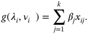
Assume that we have a random sample YT = (y1, y2, … , yn) of size n with components distributed like y, i.e. they have the same parameters λ, ν. We further assume that yi depends on regressor variables (xi0, xi1, … , xik) influencing the link function g(λi, νi), i = 1, …, n via
Without loss of generality we use the inverse link function ![]() in place of the canonical link function in the denominator. That there is no loss of generality stems from the fact that
in place of the canonical link function in the denominator. That there is no loss of generality stems from the fact that


11.8 GLM for Gamma Regression
11.9 GLM for the Multinomial Distribution
The multinomial logit model is a generalisation of the binomial logit model. It describes an (m − 1)‐dimensional response variable ![]() occurring with probabilities
occurring with probabilities ![]() . The probability (likelihood) function of the multinomial distribution is
. The probability (likelihood) function of the multinomial distribution is


The relation between the regressor variables (x0, x1, … , xk) and the probabilities pi is described by the multinomial logit function as link function

where p1 is the probability of the reference category.
The model is fitted as described in Section 11.6.1 for the Poisson model because we have an equivalence between the multinomial distribution and a Poisson distribution with fixed sum of all counts.
References
- Agresti, A. (2018). Categorical Data Analysis. New York: Wiley.
- von Bortkiewicz, L.J. (1893). Die mittlere Lebensdauer. Die Methoden ihrer Bestimmung und ihr Verhältnis zur Sterblichkeitsmessung. Jena: Gustav Fischer.
- Collett, D. (1991). Modelling Binary Data. Boca Raton: Chapman & Hall.
- Faraway, J.J. (2016). Extending the Linear Model with R: Generalized Linear, Mixed Effects and Nonparametric Regression Models, 2e. Boca Raton: Chapman & Hall/CRC Texts in Statistical Science.
- McCullagh, P. and Nelder, J.A. (1989). Generalized Linear Models. New York: Springer.
- Myers, R.H. and Montgomery, D.C. (1997). A tutorial on generalized linear models. J. Qual. Technol. 29: 274–291, (Published online: 21 Feb 2018).
- Nelder, J.A. and Wedderburn, R.W.M. (1972). Generalized linear models. J. R. Stat. Soc. 135: 370–384.
- Rasch, G. (1960). Probabilistic Models for Some Intelligence and Attainment Tests. Kopenhagen: Nissen & Lydicke.
- Rasch, G. (1980). Probabilistic Models for Some Intelligence and Attainment Tests. Danish Institute for Educational Research, Copenhagen 1960, expanded edition with foreword and afterword by B.D. Wright. Chicago: The University of Chicago Press.
- Rasch, D. and Schott, D. (2018). Mathematical Statistics. Oxford: Wiley.
- Rasch, D., Herrendörfer, G., Bock, J. et al. (1998). Verfahrensbibliothek Versuchsplanung und ‐ auswertung, 2. verbesserte Auflage in einem Band mit CD. München Wien: R. Oldenbourg Verlag.