Search in book...
Toggle Font Controls
Create new playlist

Name your new playlist

Playlist description (optional)
Sign In

Email address

Password

Forgot Password?

or

Continue with Facebook

Continue with Google
Sign Up

Full Name

Email address

Confirm Email Address

Password

or

Continue with Facebook

Continue with Google

4
Confidence Estimations – One‐ and Two‐Sample Problems

4.1 Introduction

In confidence estimation, we construct random regions in the parameter space so that this region covers the unknown parameter with a given probability, the confidence coefficient. In this book we consider special regions, namely intervals called confidence intervals. We then speak about interval estimation. We will see that there are analogies to the test theory concerning the optimality of confidence intervals, which we exploit to simplify many considerations.

A confidence interval is a function of the random sample; that is to say, it is also random in the sense of depending on chance, hence we speak of a random interval. However, once calculated based on observations, the interval has, of course, non‐random bounds. Sometimes only one of the bounds is of interest; the other is then fixed – this concerns the estimator as well as the estimate itself. At least one boundary of a confidence interval must be random; if both boundaries are random, the interval is two‐sided, and if only one boundary is random, it is one‐sided.

We make no difference between a random interval and its realisation with real boundaries but speak always about confidence intervals. What we mean in special cases will be easy to understand. When we speak about the expected length of a confidence interval, we of course mean a random interval.

Definition 4.1

Let Y = (y₁, y₂, … , y_n)^T be a random sample with realisations Y ε {Y}, whose components are distributed with a parameter θ ε Ω. Let K(Y) be a random set with realisations K(Y) in Ω. K(Y) is said to be a confidence region for θ with the corresponding confidence coefficient (confidence level) 1 − α if

4.1

In condensed form K(Y) is also said to be a (1 − α) confidence region. If Ω ⊂ R¹ and K(Y) is a connected set for all Y ε {Y}, then K(Y) is a (1 − α) confidence interval. The realisation K(Y) of a confidence region is called a realised confidence region.

Statistical tests and confidence estimations for normal distributions are extremely robust against the violation of the normality assumption, as was shown by simulation – see Rasch and Tiku (1985).

4.2 The One‐Sample Case

We start with normal distributions and confidence intervals for the expectation.

4.2.1 A Confidence Interval for the Expectation of a Normal Distribution

Problem 4.1

Construct a one‐sided (1 − α) confidence interval for the expectation of a N(μ, σ²) distribution if the variance is known.

Solution

Let the n > 1 components of a random sample Y = (y₁, y₂, … , y_n)^T be distributed as N(μ,σ²), where σ² is known. The mean follows a N(μ, ) distribution. A (1 − α) confidence interval K(Y) with respect to μ has to satisfy P[μ ε K(Y)] = 1 − α . This means (with as the random lower bound and as the random upper bound) in the case of a two‐sided (1 − α) confidence interval

Since is distributed as N(μ,), it holds that

for α₁ + α₂ = α, α₁ ≥ 0, α₂ ≥ 0. Consequently, we have

4.2

so that and is fulfilled. For 1 − α there are infinitely many confidence intervals according to the choice of α₁ and α₂ = α − α₁. If α₁ = 0 or α₂ = 0, respectively, then the confidence intervals are one‐sided (i.e. only one interval bound is random). The more the values α₁ and α₂ differ from each other, the larger the expected width = . For example, the width becomes infinite for α₁ = 0 or for α₂ = 0. Finite confidence intervals result for α₁ > 0, α₂ > 0 and an optimal choice is .

In the case of a one‐sided (1 − α) confidence interval we have either

for the left‐sided interval or
for the right‐sided interval.

From this, it follows either

4.3

4.4

Example

We construct in R a realised left‐sided and right‐sided 0.95 and a 0.99 confidence interval for the normally distributed random sample of x‐data in Table 3.4 assuming that the variance is known as σ² = 1.

 > x <- c(7.6, 13.2, 9.1, 10.6, 8.7, 10.6, 6.8, 9.9, 7.3, 10.4,
         13.3, 10.0, 9.5)
> xbar <- mean(x) 
> var <- 1
> sdx <- sqrt(var/length(x))
> conf.level <- 0.95
> z <- qnorm(1-conf.level, lower.tail=FALSE)
> xl <- xbar -z*sdx  # lower 0.95-confidence limit
> xl
[1] 9.31303
> xu <- xbar + z*sdx  # upper 0.95-confidence limit
> xu
[1] 10.22543
> conf.level <- 0.99
> z <- qnorm(1-conf.level, lower.tail=FALSE)
> xl <- xbar -z*sdx  # lower 0.99-confidence limit
> xl
[1] 9.124018
> xu <- xbar + z*sdx  # upper 0.99-confidence limit
> xu
[1] 10.41444

Problem 4.2

Construct a two‐sided (1 − α) confidence interval for the expectation of a N(μ, σ²) distribution if the variance is known.

Solution

We see from the solution of Problem 4.1 the connection between a confidence interval and a statistical test.

is the test statistic (3.1) for testing the null hypothesis H₀ : μ = μ₀ against a two‐sided alternative H_A : μ = μ₁ ≠ μ₀.

From (4.2) we find that the upper bound equals and the lower bound equals the difference is . This difference is a minimum for and then equals .

Example

We construct a realised two‐sided 0.95 and a 0.99 confidence interval using R. We assume that the sample of x‐data in Table 3.4 stems from a normal distribution with known variance σ² = 1.

 > x <- c(7.6, 13.2, 9.1, 10.6, 8.7, 10.6, 6.8, 9.9, 7.3,  10.4, +13.3, 10.0, 9.5 )
> # we make a function to construct a normal two-sided + confidence-interval 
> norm.confinterval = function(data, variance = var.data,  conf.level = conf) {  z = qnorm((1 - conf.level)/2, lower.tail = FALSE) xbar = mean(data)
     sdx = sqrt(variance/length(data)) c(xbar - z * sdx, xbar + z * sdx)  }
> # confidence interval with confidence-coefficient 0.95
> norm.confinterval(x, 1, 0.95)
[1]  9.225635 10.312827
> # confidence interval with confidence-coefficient 0.99
> norm.confinterval(x, 1, 0.99)
[1]  9.054824 10.483637

We have already used the term ‘expected length’ of a two‐sided confidence interval as the expectation of the difference between the upper and the lower bound of the interval. We give now a definition.

Problem 4.3

Determine the minimal sample size for constructing a two‐sided (1 − α) confidence interval for the expectation μ of a normally distributed random variable with known variance σ² so that the expected length L is below 2δ.

Solution

From (4.2) we find that the upper bound equals and the lower bound equals the difference is . This difference is a minimum for and then equals . This is one of the very rare cases in which the length is not random and we must not determine its expectation. Because we obtain .

Our precision requirement was or, equivalently, ; i.e.

4.6

If we compare with (3.5) images we see that (4.6) equals (3.5) for Z(β₀) = 0 and this is the case for β₀ = 0.5 (the 50%‐quantile for the standard normal distribution is 0). Therefore, we can also use formulae and R‐commands for the sample size determination of tests for the confidence estimation.

Example

For a given confidence coefficient 1 − α = 0.95 the sample size n has to be determined so that the half‐expected length is δ = 0.6 σ in the one‐ and also in the two‐sided case.

One‐sided case:

Two‐sided case:

In R we use the commands:

 > Z0.95 <- qnorm(0.95)
> Z0.95
[1] 1.644854
> n_onesided <- ceiling((Z0.95/0.6)^2)
> n_onesided
[1] 8
> Z0.975 <- qnorm(0.975)
> Z0.975
[1] 1.959964
> n_twosided <- ceiling((Z0.975/0.6)^2)
> n_twosided
[1] 11

Remark

When we construct confidence intervals for location parameters, the factor two always occurs in the formula of the expected length. We therefore replace the expected length by the half‐expected length, which is better comparable with the precision requirement for one‐sided intervals in Definition 4.2.

Problem 4.4

Determine the minimal sample size for constructing a one‐sided (1 − α) confidence interval for the expectation μ of a normally distributed random variable with known variance σ² so that the distance between the finite (random) bound of the interval and 0 is below δ.

Solution

From (4.3) and (4.4) we find that the distance of the finite bound and μ equals . The expectation of this distance is is and from this gives

4.7

Example

For a given confidence coefficient 1 − α = 0.95 the sample size n has to be determined so that the expected distance between the upper bound and μ of a one‐sided (1 − α) confidence interval is below δ = 0.6σ.

From (4.7) we obtain

In addition, this is exactly the solution of the one‐sided part given in the example of Problem 4.3.

Now we discuss the practically more interesting case that the variance is unknown. We assume that the elements of the random sample are N(μ, σ²) distributed but σ² is unknown. From (3.6) we know that

is non‐centrally t‐distributed with n − 1 degrees of freedom and non‐centrality parameter . We estimate σ by the estimator s or the realisation (the estimate) s. Analogously to (4.2) we obtain

It can be shown (Rasch and Schott (2018)) that the expected length of such an interval is minimum if we put . From this an optimal two‐sided (1 − α) confidence interval is given by

4.8

The one‐sided (1 − α) confidence intervals are given by

4.9

and

4.10

Problem 4.5

Construct a realised left‐sided 0.95 confidence interval of μ for the x‐data in Table 3.4.

Solution

Use the R command > t.test(x, alternative = "less", conf.level = 0.95).

Example

 > x <-c(7.6, 13.2, 9.1, 10.6, 8.7, 10.6, 6.8, 9.9, 7.3, 
     10.4,13)
>  t.test(x, alternative = "less", conf.level = 0.95)
      One Sample t-test data:  x
t = 17.7289, df = 12, p-value = 1
alternative hypothesis: true mean is less than 0
95 percent confidence interval:
     -Inf 10.75133
sample estimates:
mean of x
 9.769231 -Inf means -∞

Problem 4.6

Construct a realised right‐sided 0.95 confidence interval for the x‐data in Table 3.4.

Solution

Use the R command > t.test(x, alternative = "greater", conf.level = 0.95).

Example

 > t.test(x, alternative = "greater", conf.level = 0.95)
       One Sample t-test data:  x
t = 17.7289, df = 12, p-value = 2.835e-10
alternative hypothesis: true mean is greater than 0
 95 percent confidence interval:
 8.787129      Inf
sample estimates:
mean of x
 9.769231

Problem 4.7

Construct a realised two‐sided 0.95 confidence interval for the x‐data in Table 3.4.

Solution

Use the R command > t.test(x, alternative = "two.sided", conf.level = 0.95).

Example

 > t.test(x, alternative = "two.sided", conf.level = 0.95)
  One Sample t-test data:  x
t = 17.7289, df = 12, p-value = 5.67e-10
alternative hypothesis: true mean is not equal to 0
95 percent confidence interval:
  8.56863 10.96983
sample estimates:
mean of x
 9.769231

The expected length of the two‐sided (1 − α) confidence interval reads

which follows from example 2.6 in Rasch and Schott (2018).

Analogously, we obtain for the one‐sided (1 − α) confidence intervals

Now we define the following precision requirements for the construction of two‐ and one‐sided (1 − α) confidence intervals:

One‐sided (1 − α) confidence interval: determine n so that
Two‐sided (1 − α) confidence intervals: determine n so that the half expected width fulfils

From the approximate formulae, we obtain the formulae for the minimum sample size as images and , respectively.

In Table 4.1 we show how good the approximate formulae are. When the values of the table are near 1, the approximation is good.

As we can see the approximation may be used for n > 18. The approximate formula is solved iteratively by starting with a value n₀ via

Example 4.1

For i = 1 and n₀ = ∞ we obtain with and α = 0.05, n₁ = ⌈1.96²⌉ = 4, images and so on. Finally, we receive this also via the optimal design of experiments (OPDOE)‐command in R:

 > size.t.test(type="one.sample",power=0.5,delta=1,sd=1, sig.level=0.01, alternative="two.sided")
[1] 10

Thus, the final value from our iteration process is n = 10. Comparing this with the entries of Table 4.1

4.2.2 A Confidence Interval for the Variance of a Normal Distribution

We again assume that the components of the random sample Y = (y₁, … , y_n)^T are N(μ, σ²) distributed with μ and σ² unknown. To construct a two‐sided (1 − α) confidence interval for σ² we use its unbiased estimator s² and use as in Chapter 3 the test statistic which is centrally χ² ‐distributed with n − 1 degrees of freedom. Therefore

4.11

However, contrary to the tests about expectations it is not optimal to split α into equal parts as reasonable for the corresponding uniformly most powerful unbiased (UMPU) test. However, the unequal case does not always give a shorter expected length and therefore we use the split of α into equal parts. From (4.11) with α₁ = α₂ = α we obtain a (1 − α) confidence interval for σ² as

4.12

The half‐expected length of this interval is images

Problem 4.8

Construct a realised two‐sided 0.95 confidence interval for σ² for the random sample of normally distributed x‐data in Table 3.4.

Solution

Here we have a random sample X of size n from N(μ, σ²) with unknown parameters μ and σ². We want to construct a two‐sided l − α confidence interval for σ² with confidence level = clalpha. We get the solution in R using the following function > var.interval.

 > var.interval = function(data, conf.level = clalpha) {
    df = length(data) - 1
    chilower = qchisq((1 - conf.level)/2, df)
    chiupper = qchisq((1 - conf.level)/2, df, lower.tail
             = FALSE)
    v = var(data)
    c(df * v/chiupper, df * v/chilower)
   }

Example

 >x <- c(7.6, 13.2, 9.1, 10.6, 8.7, 10.6, 6.8, 9.9, 7.3, 10.4,
         13.3, 10.0, 9.5 )
> var.interval(x, 0.95)
[1]  2.029754 10.756123

Problem 4.9

Determine the sample size for constructing a (1 − α) confidence interval for the variance σ² of a normal distribution so that

(a) or
(b) .

Solution

Use the OPDOE‐command in R >size.variance.confint(alpha=,delta=) in case (a) or >size.variance.confint(alpha=,deltarel=) in case (b).

Example

We use (1 − α) = 0.9 and δ_rel = δ = 0.3 and get in case (a) with σ² = 1

 > size.variance.confint(alpha=0.1,delta=0.3)$n
[1] 67

and in case (b)

 > size.variance.confint(alpha=0.1,deltarel=0.3)$n
[1] 59

4.2.3 A Confidence Interval for a Probability

Let us presume n independent trials in each of which a certain event A occurs with the same probability p. A (1 − α) confidence interval for p can be calculated from the number of occurrences y of the event A under the n observations as [l(n,y,α); u(n,y,α)], with the lower bound l(n,y,α) and the upper bound, u(n,y,α), respectively given by:

4.13

4.14

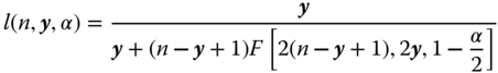
F(f₁, f₂, P) is the P‐quantile of an F‐distribution with f₁ and f₂ degrees of freedom.

For other interval estimators of a binomial proportion see Pires and Amado (2008).

To determine the minimum sample size approximately, it seems better to use the half‐expected width of a normal approximated confidence interval for p. Such an interval is given by

4.15

This interval has an approximate half‐expected width . The requirement that this is smaller than δ leads to the sample size

If nothing is known about p, we must take into account the least favourable case p = 0.5, which gives the maximum of the minimal sample size, the maximum size.

Problem 4.10

Compare the realised exact interval with the realised bounds (4.13) and (4.14) with the realised approximate interval (4.15).

Solution

Use the R‐program

 > binom.test(x,n, p=0.5, alternative = c("two.sided", "less",
      "greater"), conf.level  = 0.95)
  x          number of successes, or a vector of length 2 giving
             the numbers of successes and failures respectively.
  n          number of trials; ignored if x has length 2.
  p          hypothesized probability of success.
 alternative    indicates the alternative hypothesis and must be
                one of "two.sided", "less" or "greater". You can
                specify just the initial letter.
 conf.level  confidence level of the returned confidence interval.

Example

For n = 20, number of successes y = 5 and α = 0.05.

Exact binomial test in R:

 > binom.test(5,20,p =0.5, alternative = "two.sided" ,
        conf.level = 0.95)
        Exact binomial test
data:  5 and 20
number of successes = 5, number of trials = 20, p-value =
 0.04139
alternative hypothesis: true probability of success is not
 equal to 0.5
95 percent confidence interval:
 0.08657147 0.49104587
sample estimates:
probability of success
                  0.25

Normal approximate interval in R.

 > n <- 20
> y <- 5
> est_p <- y/n
> est_p
[1] 0.25
> z_0.975 <- qnorm(0.975)
> z_0.975
[1] 1.959964
> n <- 20
> half_width <- z_0.975* sqrt((est_p*(1-est_p)/n))
> half_width
[1] 0.1897727
> lowerCL <- est_p - half_width
> upperCL <- est_p + half_width
> CL <- c(lowerCL, upperCL)
> CL
[1] 0.0602273 0.4397727

We get with the exact result for CL (0.086 571 47; 0.491 045 87) and with the normal approximation for CL (0.060 227 3; 0.439 772 7).

Problem 4.11

Determine the sample size for the approximate interval (4.15).

Solution

Use the OPDOE‐command in R >size.prop.confint(p=,delta=,alpha=).

Example

We require a confidence interval for the probability p = P(A) of the event A: ‘an iron casting is faulty’. The confidence coefficient is specified as 0.90. How many castings should be tested if the half‐expected width of the interval is:

(a) Not greater than δ = 0.15, and nothing is known about p?
(b) Not greater than δ = 0.15, when we know that at most 10% of castings are faulty?
We use the command above and obtain:

(a) > size.prop.confint(p=0.5,delta=0.15,alpha=0.05)

[1] 43

(b) > size.prop.confint(p=0.1,delta=0.15,alpha=0.05)

[1] 16

As we can see, the maximum size is much larger than the size using prior information. Even if p = 0.3 we spare some observations.

 > size.prop.confint(p=0.3,delta=0.15,alpha=0.05)
[1] 36

4.3 The Two‐Sample Case

We discuss here only differences between location parameters of two populations; for variances we had to consider ratios but the reader can derive the corresponding intervals using the approach described for differences. We assume that the character of interest in each population is modelled by a normally distributed random variable. That is to say, we draw independent random samples of size n₁ and n₂, respectively, from populations 1 and 2. The observations of the random variables y₁₁, y₁₂, … , on the one hand and y₂₁, y₂₂, … , on the other hand will be y₁₁, y₁₂, … , and y₂₁, y₂₂, … , . We call the underlying parameters μ₁ and μ₂, respectively, and further and , respectively. The unbiased estimators are then for the expectations and , respectively, and for the variances and , respectively (according to Section 3.2).

4.3.1 A Confidence Interval for the Difference of Two Expectations – Equal Variances

If in the two‐sample case the two variances are equal, usually from the two samples y₁₁, y₁₂, … , and y₂₁, y₂₂, … , a pooled estimator of the common variance σ² is calculated.

The two‐sided confidence interval is

4.16

The lower (1 − α) confidence interval is given by

and the upper one by

Problem 4.12

Calculate the confidence interval (4.16).

Solution

In R use:

  > t.test(x, alternative= "two.sided", var.equal=TRUE,
      conf.level = 0.95)

Example

 > x <- c(7.6, 13.2, 9.1, 10.6, 8.7, 10.6, 6.8, 9.9, 7.3,  10.4, 13.3, 10.0, 9.5 )
> t.test(x, alternative= "two.sided", var.equal=TRUE,
        conf.level = 0.95)
        One Sample t-test
data:  x
t = 17.7289, df = 12, p-value = 5.67e-10
alternative hypothesis: true mean is not equal to 0
95 percent confidence interval:
  8.56863 10.96983
sample estimates:
mean of x
 9.769231

In the case of equal variances, it can be shown that optimal plans require equal sample sizes n_x and n_y. Thus n_x = n_y = n, and in the case where the half‐expected width must be less than δ, we find n iteratively from

4.17

The reader may derive the sample size needed for one‐sided intervals.

Problem 4.13

Calculate n using (4.17).

Solution

Use

 > size.t.test(power=0.5,sig.level=,delta=,sd=, type =
      "two.sample")

Example

We calculate the sample size for α = 0.05, δ = 0.5, sd = 1.

 > size.t.test(power=0.5,sig.level=0.05,delta=0.5,sd=1,type =
     "two.sample")
[1] 32

Problem 4.14

Derive the sample size formula for the construction of a one‐sided confidence interval for the difference between two expectations for equal variances.

Solution

Analogously to (4.17) we obtain the formula

and the corresponding R‐command

 > size.t.test(power=0.5,sig.level=,delta=,sd=,
    type="one.sample")

Example

We calculate the sample size for α = 0.05, δ = 0.5, sd = 1.

 > size.t.test(power=0.5,sig.level=0.05,delta=0.5,sd=1,type =
    "one.sample")
[1] 18

We see that the sample size for a one‐sided confidence interval with an analogous precision requirement as for the two‐sided case is smaller than that for the two‐sided case.

4.3.2 A Confidence Interval for the Difference of Two Expectations – Unequal Variances

If in the two‐sample case, the two variances and are unequal, sample variances and from the two independent samples y₁₁, y₁₂, … , and y₂₁, y₂₂, … , are used.

The confidence interval

4.18

is an approximate (1 − α) confidence interval (Welch 1947) with images degrees of freedom.

Example 4.2

Using R, determine a realised two‐sided 0.95 confidence interval of μ for the random samples of normally distributed x‐ and y‐data in Table 3.4. We assume that there are two independent random samples of the mice populations.

 > x <- c(7.6, 13.2, 9.1, 10.6, 8.7, 10.6, 6.8, 9.9, 7.3, 10.4, 13.3, 10.0, 9.5)
> y <- c(7.8, 11.1, 16.4, 13.7, 10.7, 12.3, 14.0, 11.9, 8.8, 7.7, 8.9, 16.4, 10.2)
> t.test(x,y,alternative = "two.sided", mu = 0,
         var.equal = FALSE, conf.level=0.95)
        Welch Two Sample t-test
data:  x and y
t = -1.7849, df = 21.021, p-value = 0.08871
alternative hypothesis: true difference in means is not
  equal to 0
95 percent confidence interval:
 -3.8137583  0.2906814
sample estimates:
mean of x mean of y
 9.769231 11.530769

To determine the necessary sample sizes n₁ and n_2, besides an upper bound for the half expected width δ, we need information about the two variances. Suppose that prior estimates and are available for the variances, which may possibly be unequal. For a two‐sided confidence interval, we can calculate n₁ and n₂ approximately (by replacing the variances by their estimates) and iteratively from

and images .

Problem 4.15

We would like to find a two‐sided 99% confidence interval for the difference of the expectations of two normal distributions with unequal variances using independent samples from each population with power = 0.90 and variance ratio σ₁²/σ₂² = 4. Given the minimum size of an experiment, we would like to find a two‐sided 99% confidence interval for the difference of the expectations of two normal distributions with unequal variances using independent samples from each population and define the precision by δ = 0.4σ_x. If we know that images , we obtain .

Solution

Use first the OPDOE‐command in R

 > power.t.test (sd = , sig.level = , delta = , power = ,  type = "two.sample", alternative = "two.sided")

This gives us the equal sample sizes due to the implementation of σ₁ = σ₂. We have assumed that / = 4, hence σ₁/σ₂ = 2.

We may conjecture that n₁ is two times as large as σ₂ because σ₁ = 2σ₂. Hence we take n₁ = 2n₂.

Example

We define the precision by α = 0.01, δ = 0.4σ, and assume that

 > power.t.test(sd=1,sig.level=0.01,delta=0.4,power = 0.9,
  type = "two.sample", alternative = "two.sided")

     Two-sample t test power calculation

              n = 187.6586
          delta = 0.4
             sd = 1
      sig.level = 0.01
          power = 0.9
    alternative = two.sided

NOTE: n is number in *each* group

Hence n₂ = 188 and n₁ = 2 * 188 = 376.

4.3.3 A Confidence Interval for the Difference of Two Probabilities

Let us say that we are interested in a certain characteristic A from the elements of a population of size N. The number of elements in this population with characteristic A is N(A). The population fraction with characteristic A is π = N(A)/N. We take a random sample of size n with replacement from this population and then the random variable k of elements with this characteristic A has a binomial distribution B(n, π) with the parameters π and n.

The sample fraction p = k/n is an unbiased estimator of π with expectation E(p) = π and variance var(p) = π(1 − π)/n. If neither k nor n − k is less than 5 and if the sample size n is large then the distribution of k can be approximated by a normal distribution with the mean μ = p, the sample fraction, and variance σ² = p(1 − p)/n.

In practice the researcher is very often interested in the difference between the population fractions with characteristic A in the two populations I and II, namely π₁ and π₂. Suppose we have a random sample of size n₁ from population I and another independent sample of size n₂ from population II. Then the unbiased estimator of π₁ − π₂ is the difference of the sample fractions p₁ − p₂. If neither k₁ nor n₁ − k₁ and k₂ nor n₂ − k₂ is less than 5 and if the sample sizes n₁ and n₂ are large then the distribution of k can be approximated by a normal distribution with mean μ = p₁ − p₂ and variance σ² = p₁(1 − p₁)/n₁ + p₂(1 − p₂)/n₂.

A confidence interval with confidence coefficient 1 − α for π₁ − π₂ is then approximated with

Example 4.3

Best et al. (1967) reported that from men aged 60–64 years at the beginning of the study, belonging to one of the two classes: (i) ‘non‐smoker’ and (ii) ‘those who reported that they smoked pipes only’, the number of deaths during the succeeding six years was obtained.

The 2 × 2 contingency table of the observations is shown in Table 4.2.

Table 4.2 Confidence table of two kinds of smokers.

	Sample 1 (non‐smokers)	Sample 2 (pipe smokers)
Dead	117	54
Alive	950	348
Total	n₁ = 1067	n₂ = 402

In R we can find the 95% confidence interval for the difference in the fraction of deceased as follows:

 > CT2x2  <- cbind(c(117, 950), c(54, 348))
> CT2x2
     [,1] [,2]
[1,]  117   54
[2,]  950  348
> n1 <- sum(CT2x2[,1])
> n1
[1] 1067
> n2 <- sum(CT2x2[,2])
> n2
[1] 402
> prop.test(x=c(117,54), n=c(1067,402))
        2-sample test for equality of proportions with continuity correction

data:  c(117, 54) out of c(1067, 402)
X-squared = 1.4969, df = 1, p-value = 0.2212
alternative hypothesis: two.sided
95 percent confidence interval:
 -0.06463259  0.01528234
sample estimates:
   prop 1    prop 2
0.1096532 0.1343284

Hence the 95% confidence interval is: −0.064 632 59 < π₁ − π₂ < 0.015 282 34.

The estimate of π₁ is p₁ = 0.109 653 2 and the estimate of π₂ is p₂ = 0.134 328 4.

Calculation with the normal approximation in R by the formula above gives:

 > p₁<-  0.1096532
> p₂<- 0.1343284
> diff <- p1- p2
> diff
[1] -0.0246752
> n1 <- 1067
> n2 <- 402
> z_0.975 = qnorm(0.975)
> z_0.975
[1] 1.959964
> width <- z_0.975*sqrt((p1*(1-p1)/n1) + (p2*(1-p2)/n2))
> width
[1] 0.03824509
> width <- z_0.975*sqrt((p1*(1-p1)/n1) + (p2*(1-p2)/n2))
> width
[1] 0.03824509
> CLlower <- diff - width
> CLlower
[1] -0.06292029
> CLupper <- diff + width
> CLupper
[1] 0.01356989

The difference in the results of the command prop.test is due to the use of Yates' continuity correction in the normal approximation, because the default command is correct = TRUE. Further defaults are alternative = "two.sided" and the default confidence level is conf.level = 0.95. The complete command is:

 > prop.test(x=c(117,54), n=c(1067,402),alternative= "two.sided",conf.level=0.95,correct=TRUE)
        2-sample test for equality of proportions with continuity correction
data:  c(117, 54) out of c(1067, 402)
X-squared = 1.4969, df = 1, p-value = 0.2212
alternative hypothesis: two.sided
95 percent confidence interval:
 -0.06463259  0.01528234
sample estimates:
   prop 1    prop 2
0.1096532 0.1343284

If we do not want to use Yates' continuity correction the command is:

 > prop.test(x=c(117,54), n=c(1067,402),alternative =
   "two.sided",  conf.level = 0.95 , correct =FALSE)
        2-sample test for equality of proportions without continuity correction
data:  c(117, 54) out of c(1067, 402)
X-squared = 1.7285, df = 1, p-value = 0.1886
alternative hypothesis: two.sided
95 percent confidence interval:
 -0.06292021  0.01356996
sample estimates:
   prop 1    prop 2
0.1096532 0.1343284

Altman et al. (2002) recommend for the two sample unpaired case a different method for the confidence interval of the difference between two population proportions.

The recommended method can also be used for small data samples. The confidence interval calculation is method 10 of Newcombe (1998). Calculate for the first random sample of size n₁ with the sample fraction p₁ the lower limit l₁ and upper limit u₁ that define the (1 − α) confidence interval for the first population proportion π₁. For the second sample of size n₂ calculate with the sample fraction p₂ the lower limit l₂ and upper limit u₂ that define the (1 − α) confidence interval for the second population proportion π₂.

The (1 − α) confidence interval for π₁ − π₂ has lower limit D − √ [(p₁ − l₁)² + (u₂ − p₂)²] and upper limit D + √ [(p₂ − l₂)² + (u₁ − p₁)²] with D = p₁ − p₂. Note that D is not generally at the midpoint of the confidence interval.

Example 4.4

Goodfield et al. (1992) reported adverse effects for dermatophyte onchomyosis (respiratory problems) for 5 patients in a random sample of 56 patients treated with terbinafine and for 0 patients in a random sample of 29 placebo treated patients.

In R we do the analysis as follows:

 > binom.test(5, 56, p =0.5, alternative = "two.sided" ,
        conf.level = 0.95)
        Exact binomial test
data:  5 and 56
number of successes = 5, number of trials = 56, p-value =
     1.17e-10
alternative hypothesis: true probability of success is not
     equal to 0.5
95 percent confidence interval:
 0.02962984  0.19619344
sample estimates:
probability of success
            0.08928571
> binom.test(0, 29, p =0.5, alternative = "two.sided" ,
   conf.level = 0.95)
        Exact binomial test
data:  0 and 29
number of successes = 0, number of trials = 29, p-value =
   3.725e-09
alternative hypothesis: true probability of success is not
   equal to 0.5
95 percent confidence interval:
 0.0000000   0.1194449
sample estimates:
probability of success
                     0

We used the results of the binom.test()in the following commands:

 > p1 <- 0.08928571
> l1 <- 0.02962984
> u1 <- 0.19619344
> p2 <-  0
> l2 <-  0.0000000
> u2 <-  0.1194449
> D <- p1-p2
> widthlower <-  sqrt((p1-l1)^2 + (u2-p2)^2)
> widthupper <- sqrt((p2-l2)^2 + (u1-p1)^2)
> CIlower <- D – widthlower
> CIupper <- D + widthupper
> CIlower
[1] -0.02970976
> CIupper
[1] 0.1961934

Hence the approximate (1 − 0.05) confidence interval is −0.029 709 76 < π₁ − π₂ < 0.196 193 4.

References

Altman, D.G., Machin, D., Bryant, T.N., and Gardner, M.J. (2002). Statistics with Confidence; Confidence Intervals and Statistical Guidelines, 2e. Bristol: British Medical Journal Books.
Best, E.W.R., Walker, C.B., Baker, P.M. et al. (1967). Summary of a Canadian Study on Smoking and Health. Can. Med. Assoc. J. 96 (15): 1104–1108.
Goodfield, M.J.D., Andrew, L., and Evans, E.G.V. (1992). Short‐term treatment of dermatophyte onchomyotis with terbinafine. BMJ 304: 1151–1154.
Newcombe, R.G. (1998). Interval estimation for the difference between independent proportions: comparison of eleven methods. Stat. Med. 17: 873–890.
Pires, A.M. and Amado, C. (2008). Interval estimators for a binomial proportion: comparison of twenty methods. RevStat Stat. J. 6 (2): 165–197.
Rasch, D. and Schott, D. (2018). Mathematical Statistics. Oxford: Wiley.
Rasch, D. and Tiku, M.L. (eds. 1985) Robustness of statistical methods and nonparametric statistics. Proc. Conf. on Robustness of Statistical Methods and Nonparametric Statistics, Schwerin (DDR), May 29 June 2, 1983. Reidel Publ. Co. Dordrecht.
Welch, B.L. (1947). The generalization of students problem when several different population variances are involved. Biometrika 34: 28–35.

..................Content has been hidden....................

You can't read the all page of ebook, please click here login for view all page.

n
2	0.797 884 6σ
3	0.886 226 9σ
4	0.921 317 7σ
5	0.939 985 6σ
6	0.951 532 9σ
7	0.959 368 8σ
8	0.965 030 5σ
9	0.972 659 3σ
10	0.972 659 3σ
11	0.975 350 1σ
12	0.977 559 4σ
13	0.979 405 6σ
14	0.980 971 4σ
15	0.982 316 2σ
16	0.983 483 5σ
17	0.984 506 4σ
18	0.985 410 0σ
19	0.986 214 1σ
20	0.986 934 3σ

Table of Contents for 4 Confidence Estimations – One‐ and Two‐Sample Problems

Create new playlist

Sign In

Sign Up

4.1 Introduction

4.2 The One‐Sample Case

4.2.1 A Confidence Interval for the Expectation of a Normal Distribution

4.2.2 A Confidence Interval for the Variance of a Normal Distribution

4.2.3 A Confidence Interval for a Probability

4.3 The Two‐Sample Case

4.3.1 A Confidence Interval for the Difference of Two Expectations – Equal Variances

4.3.2 A Confidence Interval for the Difference of Two Expectations – Unequal Variances

4.3.3 A Confidence Interval for the Difference of Two Probabilities

References

Table of Contents for
4 Confidence Estimations – One‐ and Two‐Sample Problems