6
Analysis of Variance – Models with Random Effects
6.1 Introduction
Whereas in Chapter 5 the general structure of analysis of variance models are introduced and investigated for the case that all effects are fixed real numbers (ANOVA model I), we now consider the same models but assume that all factor levels have randomly been drawn from a universe of factor levels. We call this the ANOVA model II. Therefore, effects (except the overall mean μ) are random variables and not parameters, which have to be estimated. Instead of estimating the random effects, we estimate and test the variances of these effects – called variance components. The terms main effect and the interaction effect are defined as in Chapter 5 (but these effects are now random variables).
6.2 One‐Way Classification
We characterise methods of variance component estimation for the simplest case, the one‐way ANOVA, and demonstrate most of them by some data set. For this, we assume that a sample of a levels of a random factor A has been drawn from the universe of factor levels, which is assumed to be large. In order to be not too abstract let us assume that the levels are sires. From the ith sire a random sample of ni daughters is drawn and their milk yield yij recorded. This case is called balanced if for each of the sires the same number n of daughters has been selected. If the ni are not all equal to n we called it an unbalanced design.
We consider the model
The ai are the main effects of the levels Ai. They are random variables. The eij are the errors and also random. The constant μ is the overall mean. Model (6.1) is completed by the assumptions
all random components on the right‐hand side of (6.1) are independent.
The variances ![]() and σ2 are called variance components. The total number of observations is always denoted by N, in the balanced case we have N = an. From (6.2) it follows
and σ2 are called variance components. The total number of observations is always denoted by N, in the balanced case we have N = an. From (6.2) it follows
Let us assume that all the random variables in (6.1) are normally distributed even if this is not needed for all the estimation methods. Then it follows that ai and eij are independent of each other N(0; σa2)‐ and N(0; σ2)‐distributed respectively. The yij are not independent of each other N(μ; σ2 + σa2)‐distributed. The dependence exists between variables within the same factor level (class) because
We call cov(yij, yik), i = 1, … , a; j = 1, … , n the covariance within classes.
A standardised measure of this dependence is the intra‐class correlation coefficient

The ANOVA table is that of Table 5.2 but the expected mean squares (MS) differ from those in Table 5.2 and are given in Table 6.1.
Table 6.1 Expected mean squares of the one‐way ANOVA model II.
| Source of variation | df | MS |
E(MS) Unbalanced case |
E(MS) Balanced case |
| Factor A | a − 1 | σ2 + 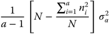 |
σ2 + |
|
| Residual | a(n − 1) | σ2 | σ2 |
6.2.1 Estimation of the Variance Components
For the one‐way classification, we describe several methods of estimation and compare them with each other. The analysis of variance method is the simplest one and stems from the originator of the analysis of variance, R. A. Fisher. In Henderson's fundamental paper from 1953, it was mentioned as method I. An estimator is defined as a random mapping from the sample space into the parameter space. The parameter space of variances and variance components is the positive real line. When realisations of such a mapping can be outside of the parameter space, we should not call them estimators. Nevertheless, this term is in use in the estimation of variance components following the citation “A good man with his groping intuitions! Still knows the path that is true and fit.” Or its German original in Goethe's Faust, Prolog. (Der Herr): “Ein guter Mensch, in seinem dunklen Drange, ist sich des rechten Weges wohl bewußt.”
We use below the notation ![]() for the vector of all observations. The variance of Y is a matrix
for the vector of all observations. The variance of Y is a matrix

6.2.1.1 ANOVA Method
The ANOVA method does not need the normal assumption; it follows in all classifications the same algorithm.
Algorithm for estimating variance components by the analysis of variance method:
- Obtain from the column E(MS) in any of the ANOVA tables (here and in the further sections) the formula for each variance component
- Replace E(MS) by MS and σ2 in the equations by the corresponding s2 to obtain the estimators or by s2 to receive the estimates of the corresponding variance components.
Because in the equations differences of MS occur it may happen that, we receive negative estimators and estimates of positive parameters of the variance components. However, the ANOVA method for estimating the variance components have for normally distributed variables Y a positive probability that negative estimators, see Verdooren (1982). Nevertheless, the estimators are unbiased and for normally distributed variables Y in the balanced case they have minimum variance (best quadratic unbiased estimators), but negative estimates are impermissible, see Verdooren (1980).
We now demonstrate that algorithm in our one‐way case.
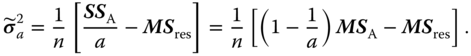
- σ2 = E(MSres),
 ,
,  , s2 = MSres;
 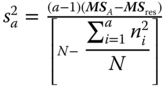 , s2 = MSres.
The estimate ![]() is negative if MSres > MSA.
is negative if MSres > MSA.
6.2.1.2 Maximum Likelihood Method
Now we use the assumption that yij in (6.1) is normally distributed with variance from (6.3). Further we assume equal sub‐class numbers, i.e. N = an because otherwise the description becomes too complicated. Those interested in the general case may read Sarhai and Ojeda (2004, 2005). Harville (1977) gives a good background of the maximum likelihood approaches.
The density function of the vector of all observations ![]() is (with ⊕ for direct sum)
is (with ⊕ for direct sum)

and this becomes

with SSres and SSA from Table 5.2.
We obtain the maximum‐likelihood – estimates ![]() ,
, ![]() , and
, and ![]() by zeroing the derivatives of ln L with respect to the three unknown parameters and obtain
by zeroing the derivatives of ln L with respect to the three unknown parameters and obtain
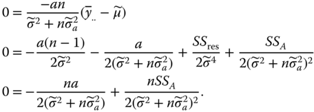
From the first equation (after transition to random variables) it follows for the estimators
and from the two other equations
and

hence
Because the matrix of the second derivatives is negative definite, we really reach maxima.
Note that for a random sample of size n from a normal variable with distribution N(μ, σ2) the maximum likelihood ML estimate of μ is the sample mean ![]() and the ML estimate for σ2 is [(n − 1)/n]s2, where s2 is the sample variance.
and the ML estimate for σ2 is [(n − 1)/n]s2, where s2 is the sample variance.
6.2.1.3 REML – Estimation
Anderson and Bancroft (1952, p. 320) introduced a restricted maximum likelihood (REML) method. There are extensions by Thompson (1962) and a generalisation by Patterson and Thompson (1971). This method uses a translation invariant restricted likelihood function depending on the variance components to be estimated only and not on the fixed effect μ. This restricted likelihood function is a function of the sufficient statistics for the variance components. The latter is then derived with respect to the variance components under the restriction that the solutions are non‐negative.
The method REML can be found in Searle et al. (1992). The method means that the likelihood function of TY is maximised in place of the likelihood function of Y. T is a (N − a − 1) × N matrix, whose rows are N − a − 1 linear independent rows of IN − X(XTX)−XT with X from 6.1 in Rasch and Schott (2018).
The (natural) logarithm of the likelihood function of TY is with V in (6.5)
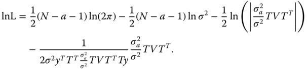
Now we differentiate this function with respect to ![]() and zeroing these derivatives. The arising equation we solve iteratively and gain the estimators.
and zeroing these derivatives. The arising equation we solve iteratively and gain the estimators.

Because the matrix of second derivatives is negative definite, we find the maxima.
Note that for a random sample of size n from a normal variable with distribution N(μ, σ2) the REML estimate of μ is the sample mean ![]() and the REML estimate for σ2 is s2, where s2 is the sample variance.
and the REML estimate for σ2 is s2, where s2 is the sample variance.
This REML method is increasingly in use in applications – especially in animal breeding; even for not normally distributed variables. Another method MINQUE (minimum norm quadratic unbiased estimator) to estimate variance components, which is not based on normally variables, needs an idea of the starting value of the variance components. Using an iterative procedure by inserting the outcomes of the previous MINQUE procedure in the next MINQUE procedure gives the same result as the REML procedure! Hence, even for not normally distributed model effects we can use the REML.
Furthermore, for balanced designs with ANOVA estimators when the estimates are not negative, the REML estimates give the same answers. If the ANOVA estimate is negative because MSA is smaller than MSres, this is an inadmissible estimate. However, the REML estimate gives in such cases the correct answer zero. Hence, in practice the REML estimators are preferred for estimating the variance components. The REML method should always be used if the data are not balanced.
Besides methods based on the frequency approach generally used in this book there are Bayesian methods of variance component estimation. In this approach, we assume that the parameters of the distribution, and by this especially the variance components, are random variables with some prior knowledge about their distribution. This prior knowledge is sometimes given by an a priori distribution, sometimes by data from an earlier experiment. This prior distribution is combined with the likelihood of the sample resulting in a posterior distribution. The estimator is used in such a way that it minimises the so‐called Bayes risk. See Tiao and Tan (1965), Federer (1968), Klotz et al. (1969), Gelman et al. (1995).
6.2.2 Tests of Hypotheses and Confidence Intervals
For the balanced one‐way random model to construct the confidence intervals for σ2a and σ2 and to tests hypotheses about these variance components we need besides (6.2) a further side condition in the model equation 6.1) about the distribution of yij. We assume now that the yij are not independent of each other ![]() ‐distributed. Then for the distribution of MSA and MSres we know from theorem 6.5 in (Rasch and Schott (2018)) that for the special case of equal sub‐class numbers (balanced case) the quadratic forms
‐distributed. Then for the distribution of MSA and MSres we know from theorem 6.5 in (Rasch and Schott (2018)) that for the special case of equal sub‐class numbers (balanced case) the quadratic forms ![]() and
and ![]() are independent of each other CS[a(n − 1)]‐ and CS[a − 1]‐ distributed, respectively. From this, it follows that
are independent of each other CS[a(n − 1)]‐ and CS[a − 1]‐ distributed, respectively. From this, it follows that

is [(σ2 + n σ2A)/σ2] F[a − 1, a(n − 1)]‐distributed. Under the null hypothesis ![]()
F is distributed as F[a − 1, a(n − 1)]. If we have for the p‐value Pr(F[a − 1, a(n − 1)] > F) ≤ α, then ![]() is rejected at significance level α.
is rejected at significance level α.
For an unbalanced design the distribution of SSA is a linear combination of (a − 1) independent CS[1] variables, where the coefficients are functions of σ2 and σ2A. Hence F is not distributed as [((σ2 + n σ2A)/σ2)]F[a − 1, a(n − 1)], but under the null hypothesis ![]() , F is distributed as F[a − 1, a(n − 1)].
, F is distributed as F[a − 1, a(n − 1)].
6.2.3 Expectation and Variances of the ANOVA Estimators
Because the estimators obtained using the ANOVA method are unbiased, we get
and
The variances and covariance of the ANOVA estimators of the variance components in the balanced case for normally distributed yij are:

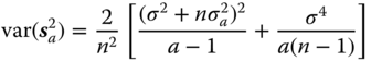

Estimators for the variances and covariance in (6.15)–(6.17) can be obtained by replacing the quantities σ2 and ![]() occurring in these formulae by their estimators s2 and
occurring in these formulae by their estimators s2 and ![]() respectively. These estimators of the variances and covariance components are biased. We get
respectively. These estimators of the variances and covariance components are biased. We get


and

6.3 Two‐Way Classification
Here and in Section 6.4, we consider mainly the estimators of the variance components with the analysis of variance method and the REML method.
6.3.1 Two‐Way Cross Classification
In the two‐way cross‐classification our model is

with side conditions that ai, bj, (a,b)ij, and eijk are uncorrelated and:

For testing and confidence intervals we additionally assume that yijk is normally distributed.
In a balanced two‐way cross‐classification (nij = n for all i, j) and normally distributed yijk the sum of squares in Table 5.7 used as a theoretical table with random variables are stochastically independent, and we have
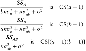
distributed.
To test the hypotheses:
we use the following facts.
The statistic

is the ![]() ‐fold of a random variable distributed as F[a − 1, (a − 1)(b − 1)]. If HA0 is true FA is F[a − 1, (a − 1)(b − 1)]‐distributed.
‐fold of a random variable distributed as F[a − 1, (a − 1)(b − 1)]. If HA0 is true FA is F[a − 1, (a − 1)(b − 1)]‐distributed.
The statistic

is the ![]() ‐fold of a random variable distributed as F[b − 1, (a − 1)(b − 1)]. If HB0 is true FB is F[b − 1, (a − 1)(b − 1)]‐distributed.
‐fold of a random variable distributed as F[b − 1, (a − 1)(b − 1)]. If HB0 is true FB is F[b − 1, (a − 1)(b − 1)]‐distributed.
The statistic

is the ![]() ‐fold of a random variable distributed as F[(a − 1)(b − 1), ab(n − 1)]. If HAB0 is true, FAB is F[(a − 1)(b − 1), ab(n − 1)]‐distributed.
‐fold of a random variable distributed as F[(a − 1)(b − 1), ab(n − 1)]. If HAB0 is true, FAB is F[(a − 1)(b − 1), ab(n − 1)]‐distributed.
The hypotheses HA0, HB0, and HAB0 are tested by the statistics FA, FB, and FAB respectively. If the observed F‐value is larger than the (1 − a)‐quantile of the central F‐distribution with the corresponding degrees of freedom we may conjecture that the corresponding variance component is positive and not zero.
6.3.2 Two‐Way Nested Classification
The two‐way nested classification is a special case of the incomplete two‐way cross‐classification, it is maximally unconnected. The formulae for the estimators of the variance components become very simple. We use the notation of Section 5.3.2, but now the ai and bj in (5.33) are random variables. The model equation (5.33) then becomes
with the conditions of uncorrelated ai, bij, and eijk and
Further, we assume for tests that the random variables ai are N(0, ![]() ), bij are N(0,
), bij are N(0, ![]() ), and eijk are N(0, σ2).
), and eijk are N(0, σ2).
We use here and in other sections the columns source of variation, sum of squares and degrees of freedom of the corresponding ANOVA tables in Chapter 5 because these columns are the same for models with fixed and random effects. The column expected mean squares and F‐test statistics must be derived for models with random effects anew. We now replace in Table 5.13 the column of E(MS) for the random model (see Table 6.6).
Table 6.6 The column E(MS) of the two‐way nested classification for model II.
| Source of variation | E(MS) |
| Between A levels | |
| Between B levels within A levels | |
| Within B levels (residual) | σ2 |
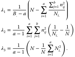
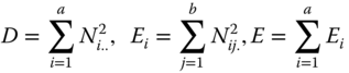
In this table the positive coefficients λi are defined by
6.4 Three‐Way Classification
We have four three‐way classifications and proceed in all sections in the same way. At first, we complete the corresponding ANOVA table of Chapter 5 using the column E(MS) for the model with random effects. Then we use the ANOVA method only and use the algorithm of the analysis of variance method in Section 6.4.1 to obtain estimators of the variance components in the balanced case.
6.4.1 Three‐Way Cross‐Classification with Equal Sub‐Class Numbers
We start with the model equation for the balanced model

with the side conditions that the expectations of all random variables of the right‐hand side of (6.27) are equal to zero and all covariances between different random variables of the right‐hand side of (6.27) vanish: var(ai) = ![]() , var(bj) =
, var(bj) = ![]() , var(ck) =
, var(ck) = ![]() , var(a,b)ij =
, var(a,b)ij = ![]() , var(a,c)ik =
, var(a,c)ik = ![]() , var(b,c)jk =
, var(b,c)jk = ![]() , var(a,b,c)ijk =
, var(a,b,c)ijk = ![]() . Further we assume for tests that the yijkl are normally distributed.
. Further we assume for tests that the yijkl are normally distributed.
Table 6.8 shows the E(MS) for this case as the new addendum of Table 5.15.
Table 6.8 The column E(MS) as supplement for model II to the analysis of variance Table 5.15.
| Source of variation | E(MS) |
| Between A levels | |
| Between B levels | |
| Between C levels | |
| Interaction A × B | |
| Interaction A × C | |
| Interaction B × C | |
| Interaction A × B × C | |
| Within the sub‐classes (residual) | σ2 |
6.4.2 Three‐Way Nested Classification
For the three‐way nested classification C ≺ B ≺ A we assume the following model equation
The conditions are: all random variables of the right‐hand side of (6.28) have expectation 0 and are pairwise uncorrelated and ![]() for all i,
for all i, ![]() for all i.j,
for all i.j, ![]() for all i, j, k and var(eijkl) = σ2 for all i, j, k, l.
for all i, j, k and var(eijkl) = σ2 for all i, j, k, l.
We find the SS, df, and MS of the three‐way nested analysis of variance in Table 5.18.
The E(MS) for the random model can be found in Table 6.11.
Table 6.11 Expectations of the MS of a three‐way nested classification for model II.
| Source of variation | E(MS) |
| Between the A levels | |
| Between the B levels within the A levels | |
| Between the C levels within the B and A levels | |
| Residual | σ2 |
In Table 6.11 we use the abbreviations:


6.4.3 Three‐Way Mixed Classifications
We consider the mixed classifications in Sections 5.5.3.1 and 5.5.3.2 but assume now random effects.
6.4.3.1 Cross‐Classification Between Two Factors Where One of Them is Sub‐Ordinated to a Third Factor ((B ≺ A)×C)
If in a balanced experiment a factor B is sub‐ordinated to a factor A and both are cross‐classified with a factor C then the corresponding model equation is given by

where μ is the general experimental mean, ai is the random effect of the ith level of factor A with E(ai) = 0, var(ai) = ![]() . Further, bij is the random effect of the jth level of factor B within the ith level of factor A, with E(bij) = 0, var(bij) =
. Further, bij is the random effect of the jth level of factor B within the ith level of factor A, with E(bij) = 0, var(bij) = ![]() and ck is the random effect of the kth level of factor C, with E(ck) = 0, var(ck) =
and ck is the random effect of the kth level of factor C, with E(ck) = 0, var(ck) = ![]() . Further, (a,c)ik and(b,c)jk(i) are the corresponding random interaction effects with E((a,c)ik) = 0, var((a,c)ik) =
. Further, (a,c)ik and(b,c)jk(i) are the corresponding random interaction effects with E((a,c)ik) = 0, var((a,c)ik) = ![]() and E((b,c)jk(i)) = 0, var ((b,c)jk(i)) =
and E((b,c)jk(i)) = 0, var ((b,c)jk(i)) = ![]() . eijkl is the random error term with E(eijkl) = 0, var (eijkl) = σ2. All the right‐hand side random effects are uncorrelated with each other.
. eijkl is the random error term with E(eijkl) = 0, var (eijkl) = σ2. All the right‐hand side random effects are uncorrelated with each other.
The ANOVA table with df and expected mean squares E(MS) is as follows, (N = abcn).
6.4.3.2 Cross‐Classification of Two Factors in Which a Third Factor is Nested (C ≺ (A×B))
The model equation for this type is
where μ is the general experimental mean, ai is the effect of the ith level of factor A with E(ai) = 0, var(ai) = ![]() . Further, bj is the effect of the jth level of factor B with E(bj) = 0, var (bj) =
. Further, bj is the effect of the jth level of factor B with E(bj) = 0, var (bj) = ![]() ; cijk is the effect of the kth level of factor C within the combinations of A × B, with E(cijk) = 0, var (cijk) =
; cijk is the effect of the kth level of factor C within the combinations of A × B, with E(cijk) = 0, var (cijk) = ![]() . Further (a,b)ij is the corresponding random interaction effect with E((a,b)ij) = 0, var ((a,b)ij) =
. Further (a,b)ij is the corresponding random interaction effect with E((a,b)ij) = 0, var ((a,b)ij) = ![]() and eijkl is the random error term with E(eijkl) = 0, var (eijkl) = σ2. The right‐hand side random effects are uncorrelated with each other.
and eijkl is the random error term with E(eijkl) = 0, var (eijkl) = σ2. The right‐hand side random effects are uncorrelated with each other.
The ANOVA table with df and expected mean squares E(MS) is as follows, (N = abcn).
References
- Anderson, R.L. and Bancroft, T.A. (1952). Statistical Theory in Research. New York: McGraw‐Hill.
- Federer, W.T. (1968). Non‐negative estimators for components of variance. Appl. Stat. 17: 171–174.
- Gaylor, D.W. and Hopper, F.N. (1969). Estimating the degree of freedom for linear combinations of mean squares by Satterthwaite's formula. Technometrics 11: 691–706.
- Gelman, A., Carlin, J.B., Stern, H.S., and Rubin, D.B. (1995). Bayesian Data Analysis. New York: Chapman and Hall.
- Hammersley, J.M. (1949). The unbiased estimate and standard error of the interclass variance. Metron 15: 189–204.
- Hartley, H.O. (1967). Expectations, variances and covariances of ANOVA mean squares by “synthesis”. Biometrics 23: 105–114.
- Harville, D.A. (1977). Maximum‐likelihood approaches to variance component estimation and to related problems. J. Am. Stat. Assoc. 72: 320–340.
- Henderson, C.R. (1953). Estimation of variance and covariance components. Biometrics 9: 226–252.
- Klotz, J.H., Milton, R.C., and Zacks, S. (1969). Mean square efficiency of estimators of variance components. J. Am. Stat. Assoc. 64: 1383–1402.
- Kuehl, R.O. (1994). Statistical Principles of Research Design and Analysis. Belmont, California: Duxbury Press.
- Patterson, H.D. and Thompson, R. (1971). Recovery of inter‐block information when block sizes are unequal. Biometrika 58: 545–554.
- Rasch, D. and Schott, D. (2018). Mathematical Statistics. Oxford: Wiley.
- Sarhai, H. and Ojeda, M.M. (2004). Analysis of Variance for Random Models, Balanced Data. Basel/Berlin: Birkhäuser, Boston.
- Sarhai, H. and Ojeda, M.M. (2005). Analysis of Variance for Random Models, Unbalanced Data. Basel/Berlin: Birkhäuser, Boston.
- Satterthwaite, F.E. (1946). An approximate distribution of estimates of variance components. Biom. Bull. 2: 110–114.
- Searle, S.R., Casella, G., and McCulloch, C.E. (1992). Variance Components. New York/Chichester/Brisbane/Toronto/Singapore: Wiley.
- Seely, J.F. and Lee, Y. (1994). A note on Satterthwaite confidence interval for a variance. Commun. Stat. 23: 859–869.
- Thompson, W.A. Jr. (1962). Negative estimates of variance components. Ann. Math. Stat. 33: 273–289.
- Tiao, G.C. and Tan, W.Y. (1965). Bayesian analysis of random effects models in the analysis of variance I: posterior distribution of variance components. Biometrika 52: 35–53.
- Townsend, E.C. (1968) Unbiased estimators of variance components in simple unbalanced designs. PhD thesis, Cornell Univ., Ithaca, USA.
- Verdooren, L.R. (1980). On estimation of variance components. Stat. Neerl. 34: 83–106.
- Verdooren, L.R. (1982). How large is the probability for the estimate of variance components to be negative? Biom. J. 24: 339–360.
- Williams, J.S. (1962). A confidence interval for variance components. Biometrika 49: 278–281.