Appendix A
List of Problems
This part of the Appendix shows the problems formulated in the chapters of this book. If we write ‘calculate’ or ‘determine’ we mean that the operations should be done using R.
Problem 1.1
Calculate the value ϕ(z) of the density function of the standard normal distribution for a given value z.Problem 1.2
Calculate the value Φ(z) of the distribution function of the standard normal distribution for a given value z.Problem 1.3
Calculate the value of the density function of the log‐normal distribution whose logarithm has mean equal tomeanlog = 0and standard deviation equal tosdlog = 1for a given value z.Problem 1.4
Calculate the value of the distribution function of the lognormal distribution whose logarithm has mean equal tomeanlog = 0and standard deviation equal tosdlog = 1for a given value z.Problem 1.5
Calculate the P%‐quantile of the t‐distribution with df degrees of freedom and optional non‐centrality parameterncp.Problem 1.6
Calculate the P%‐quantile of the χ2‐distribution with df degrees of freedom and optional non‐centrality parameterncp.Problem 1.7
Calculate the P%‐quantile of the F‐distribution with df1 and df2 degrees of freedom and optional non‐centrality parameterncp.Problem 1.8
Draw a pure random sample without replacement of size n < N from N given objects represented by numbers 1,…, N without replacing the drawn objects. There are M = possible unordered samples having the same probability p =
  to be selected.
Problem 1.9
Draw a pure random sample with replacement of size n from N given objects represented by numbers 1,…,N with replacing the drawn objects. There are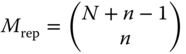 possible unordered samples having the same probability
  to be selected.
Problem 1.10
From a set of N objects systematic sampling with random start should choose a random sample of size n.Problem 1.11
By cluster sampling from a population of size N decomposed into s disjoint subpopulations, so‐called clusters of sizes N1, N2, . . , Ns a random sample should be drawn.Problem 1.12
Draw a random sample of size n in a two‐stage procedure by selecting first from the s primary units having sizes Ni (i = 1,…,s) exactly r units.Problem 2.1
Calculate the arithmetic mean of a sample.Problem 2.2
Calculate the extreme values y(1) = min(y) and y(n) = max(y) of a sample.Problem 2.3
Order a vector of numbers by magnitude.Problem 2.4
Calculate the ‐trimmed mean of a sample.
Problem 2.5
Calculate the ‐Winsorised mean of a sample of size n.
Problem 2.6
Calculate the median of a sample.Problem 2.7
Calculate the first and the third quartile of a sample.Problem 2.8
Calculate the geometric mean of a sample.Problem 2.9
Calculate the harmonic mean of a sample.Problem 2.10
Calculate from n observations (x1, x2, … , xn) of a lognormal distributed random variable the maximum‐likelihood (ML) estimate of the expectation .
.Problem 2.11
Estimate the parameter p of a binomial distributionProblem 2.12
Estimate the parameter λ of a Poisson distribution.Problem 2.13
Estimate the expectation and the variance of the initial N(μ, σ2)‐distribution after an ‘ in a’ left‐sided and after an ‘ in b’ right‐sided truncation.Problem 2.14
Estimate the expectation of a N(μ, σ2)‐distribution based on a left sided or a right‐sided censored sample of type I.Problem 2.15
The expectation μ of a of finite population is to be estimated from the realisation of a pure random sample or a systematic sampling with random start. Give the estimates of the unbiased estimator for μ and of the estimator of the standard error of the estimator of μ.Problem 2.16
A universe of size N is subdivided into s disjoint clusters of size Ni (i = 1, 2, … , s). ni sample units are drawn from stratum i by pure random sampling with a total sample size in the universe. Estimate the expectation of the universe if the ni/n are chosen proportional to Ni/N.
Problem 2.17
Estimate the expectation of a universe with N elements in s primary units (strata) having sizes Ni (i = 1,…,s) by two‐stage sampling, drawing at first r < s strata and then from each of the selected strata m elements.Problem 2.18
Calculate the range R of a sample.Problem 2.19
Calculate the interquartile range IQR(y) of a sample Y.Problem 2.20
Calculate for an observed sample the estimate (realisation) of the square root s of s2 in (2.21).Further give the estimate
 .
.Problem 2.21
Calculate the sample skewness g1 from a sample y for the data with weight 1.Problem 2.22
Calculate the sample kurtosis from a sample Y.Problem 2.23
Calculate the association measure Q in (2.26) for Example CT2x2.Problem 2.24
Calculate the association measure Y in (2.27) for Example CT2x2.Problem 2.25
Calculate the association measure H in (2.28) for Example CT2x2.Problem 2.26
Calculate χ2 and the association measure C in (2.30) for Example 2.2.Problem 2.27
Calculate the association measure Cadj in (2.31) for Example 2.2.Problem 2.28
Calculate the association measure T in (2.29) for Example 2.3.Problem 2.29
Calculate the association measure V in (2.33) for Example 2.3.Problem 3.1
Determine the P‐quantile Z(P) of the standard normal distribution.Problem 3.2
Calculate the power function of the one‐sided test for (3.3) case (a).Problem 3.3
To test H0 : μ = μ0 for a given risk of the first kind α the sample size n has to be determined so that the second kind risk β is not larger than β0 as long as μ1 − μ0≥ δ with σ = 1 in the one‐ and two‐sided case described above.Problem 3.4
Calculate the minimal sample size for testing the null hypothesis with σ = 1:- H0 : μ = μ 0 against one of the following alternative hypotheses:
- HA : μ > μ0 (one‐sided alternative),
- HA : μ ≠ μ0 (two‐sided alternative).
- H0 : μ = μ 0 against one of the following alternative hypotheses:
Problem 3.5
Let y be binomially distributed (as B(n,p)). Describe an α‐test for H0 : p = p0 against HA : p = pA < p0 and for H0 : p = p0 against HA : p = pA > p0.Problem 3.6
Let P be the family of Poisson distributions and Y = (y1, … ,yn)T a realisation of a random sample Y = (y1, … ,yn)T. The likelihood function is
How can we test the pair Ho: λ = λo, HA : λ ≠λo of hypotheses with a first kind risk α?
Problem 3.7
Perform a Wilcoxon's signed‐ranks test for a sample y.Problem 3.8
Perform a Wilcoxon's signed‐ranks test for two paired samples X and Y.Problem 3.9
Show how, based on sample values Y, the null hypothesis can be tested.
Problem 3.10
Show how a triangular sequential test can be calculated.Problem 3.11
How can we calculate the minimum sample size n per sample for the two‐sample t‐test for a risk of the first kind α and a risk of the second kind not larger than β as long as |μ1 − μ2| > δ with σ = 1?Problem 3.12
Use the Welch test based on the approximate test statistic to test- H0 : μ1 = μ2 = μ; against one of the alternative hypotheses:
- HA : μ1 < μ2,
- HA : μ1 > μ2,
- HA : μ1 ≠ μ2.
- H0 : μ1 = μ2 = μ; against one of the alternative hypotheses:
Problem 3.13
Test for two continuous distributions- H0 : m1 = m2 = m; against one of the alternative hypotheses:
- HA : m1 < m2,
- HA : m1 > m2,
- HA : m1 ≠ m2..
- H0 : m1 = m2 = m; against one of the alternative hypotheses:
Problem 3.14
Show how a triangular sequential two‐sample test is calculated.Problem 4.1
Construct a one‐sided (1 − α)‐confidence interval for the expectation of a N(μ, σ2)‐distribution if the variance is known.Problem 4.2
Construct a two‐sided (1 − α)‐confidence interval for the expectation of a N(μ, σ2)‐distribution if the variance is known.Problem 4.3
Determine the minimal sample size for constructing a two‐sided (1 − α)‐confidence interval for the expectation μ of a normally distributed random variable with known variance σ2 so that the expected length L is below 2δ.Problem 4.4
Determine the minimal sample size for constructing a one‐sided (1 − α)‐confidence interval for the expectation μ of a normally distributed random variable with known variance σ2 so that the distance between the finite (random) bound of the interval and 0 is below δ.Problem 4.5
Construct a realised left‐sided 0.95‐confidence interval of μ for the x‐data in Table 3.4.Problem 4.6
Construct a realised right‐sided 0.95‐confidence interval for the x‐data in Table 3.4.Problem 4.7
Construct a realised two‐sided 0.95‐confidence interval for the x‐data in Table 3.4.Problem 4.8
Construct a realised two‐sided 0.95‐confidence interval for σ2 for the random sample of normally distributed x‐data in Table 3.4.Problem 4.9
(a) (b) Determine the sample size for constructing a (1 − α)‐confidence interval for the variance σ2 of a normally distribution so that- (a)
 or
or - (b)
 .
.
- (a)
Problem 4.10
Compare the realised exact interval with the realised bounds (4.13) and (4.14) with the realised approximate interval (4.15).Problem 4.11
Determine the sample size for the approximate interval (4.15).Problem 4.12
Calculate the confidence interval (4.16).Problem 4.13
Calculate n with (4.17).Problem 4.14
Derive the sample size formula for the construction of a one‐sided confidence interval for the difference between two expectations for equal variances.Problem 4.15
We would like to find a two‐sided 99% confidence interval for the difference of the expectations of two normal distributions with unequal variances using independent samples from each population with power = 0.90 and variances /
/ = 4. Given the minimum size of an experiment, we would like to find a two‐sided 99% confidence interval for the difference of the expectations of two normal distributions with unequal variances using independent samples from each population and define the precision by δ = 0.4σx. If we know that
  , we obtain
  .
.Problem 5.1
Determine in a balanced design the sub‐class number n in a one‐way ANOVA for a precision determined by α = 0.05, β = 0.05 and δ = 2σ, and a test with (5.14).Problem 5.2
Calculate the entries in the ANOVA Table 5.3 and calculate estimates of (5.9) and (5.10).Problem 5.3
Test the null hypothesis H0 : a1 = a2 = a3 = 0 with significance level α = 0.05.Problem 5.4
Determine the (1 − α)‐quantile of the central F‐distribution with df1 and df2 degrees of freedom.Problem 5.5
Determine the sample size for testing HA0 : a1 = a2 = … = aa = 0.Problem 5.6
Calculate the entries of Table 5.11 and give the commands for Table 5.12.Problem 5.7
Calculate the sample size for testing HAA0 : (a, b)11 = (a, b)12 = … = (a, b)ab = 0.Problem 5.8
Calculate the ANOVA table with the realised sum of squares of Table 5.14.Problem 5.9
Determine the sub‐class number for fixed precision to test HA0 : a1 = a2 = … = aa = 0 and HB0 : b1 = b2 = … = bb = 0.Problem 5.10
Calculate the ANOVA‐table of a three‐way cross‐classification for model (5.30).Problem 5.11
Calculate the minimal sub‐class number to test hypotheses of main effect and interactions in a three‐way cross classification under model (5.30).Problem 5.12
Calculate the ANOVA table for the data of Table 5.20.Problem 5.13
Determine the minimal sub‐class numbers for the three tests of the main effects.Problem 5.14
Calculate the empirical ANOVA‐table and perform all possible F‐tests for Example 5.20.Problem 5.15
Determine the minimin and maximin sample sizes for testing HA0 : ai = 0 (for all i).Problem 5.16
Determine the minimin and maximin sample sizes for testing HC0 : ck = 0 (for all k).Problem 5.17
Determine the minimin and maximin sample sizes for testing HAxC0 : (ac)ik = 0 (for all i and k).Problem 5.18
Calculate the ANOVA table and the F‐tests for Example 5.21.Problem 5.19
Determine the minimin and maximin sample sizes for testing HA0 : ai = 0 (for all i).Problem 5.20
Determine the minimin and maximin sample sizes for testing HAxC0 : (ac)ik = 0 (for all i and k).Problem 6.1
Estimate the variance components with the ANOVA method.Problem 6.2
Estimate the variance components with the ML method.Problem 6.3
Estimate the variance components using the REML method.Problem 6.4
Test the null hypothesis for the balanced case with significance level α = 0.05.
Problem 6.5
Test the null hypothesis for the unbalanced case with significance level α = 0.05.
Problem 6.6
Construct a (1 − α)‐confidence interval for and a (1 − α)‐confidence interval for the intra‐class correlation coefficient (ICC)
  with α = 0.05.
Problem 6.7
Estimate the variance of the ANOVA estimators of the variance components σ2 and .
.Problem 6.8
Test for the balanced case the hypotheses:
with significance level α = 0.05 for each hypothesis.
Problem 6.9
Derive the estimates of the variance components with the ANOVA method and using the REML.Problem 6.10
Derive the ANOVA estimates for all variance components; give also the REML estimates.Problem 6.11
Test the hypotheses and
and  with α = 0.05 for each hypothesis.
Problem 6.12
Use the analysis of variance method to obtain the estimators for the variance components by solving
Problem 6.13
Derive the F‐tests with significance level α = 0.05 for testing each of the null hypotheses .
.Problem 6.14
Derive the approximate F‐tests with significance level α = 0.05 for testing each of the null hypotheses .
.Problem 6.15
Derive by the analysis of variance method the ANOVA estimates of the variance components in Table 6.11 and also the REML estimates.Problem 6.16
Derive by the analysis of variance method the ANOVA estimates of the variance components in Table 6.13 and also the REML estimates.Problem 6.17
Derive by the analysis of variance method the ANOVA estimates of the variance components in Table 6.15 and also the REML estimates.Problem 7.1
Derive the analysis of variance (ANOVA) estimators of all variance components using case I in the fourth column of Table 7.1.Problem 7.2
Derive the ANOVA estimators of all variance components using Case II in the last column of Table 7.1.Problem 7.3
Test H01 :“All ai are equal” against HA1 : “Not all ai are equal” with significance level α = 0.05.Problem 7.4
Show the F‐statistics and their degrees of freedom to test H02: ‘ = 0’ and H03: ‘
 = 0’, each with significance level α = 0.05.
Problem 7.5
Estimate the variance components in an unbalanced two‐way mixed model for Example 7.2.Problem 7.6
Determine the minimin and maximin number of levels of the random factor to test H01: ‘all ai are zero’ if no interactions are expected for given values of α, β, δ/σ, a and n.Problem 7.7
Determine the minimin and maximin number of levels of the random factor to test H01: “all ai are equal” if interactions are expected.Problem 7.8
Estimate the variance components if the nested factor B is random by the ANOVA method.Problem 7.9
How can we test the null hypothesis that the effects of all the levels of factor A are equal, H0A: “all ai are equal” against HaA: “not all ai are equal”, with significance level α = 0.05?Problem 7.10
How can we test the null hypothesis against HBA:
  > 0 with significance level α = 0.05?
Problem 7.11
Find the minimum size of the experiment which for a given number a of levels of the factor A will satisfy the precision requirements given by α; β, δ, σ.Problem 7.12
Estimate the variance components σ2 and by the analysis of variance method.
Problem 7.13
Test the null hypothesis HB0:“the effects of all the levels of factor B are equal” against HB0: “the effects of all the levels of factor B are not equal” with significance level α = 0.05.Problem 7.14
Test the null hypothesis against HAA:
  > 0 with significance level α = 0.05.
Problem 7.15
Show how we can determine the minimin and the maximin sample size to test the null hypothesis .
.Problem 7.16
Use the algorithm above to find the test statistic for testing HA0 : ai = 0, ∀ i against HAA : “at least one ai ≠ 0” for model III.Problem 7.17
Use the algorithm above to find the test statistic for testing HB0 : bj = 0, ∀ j against HBA : “at least one bj ≠ 0” for model III.Problem 7.18
Use the algorithm above to find the test statistic for testing HAB0 : (ab)ij = 0, ∀ i, j against HABA : “at least one (ab)ij ≠ 0” for model III.Problem 7.19
The minimin and maximin number of levels of the random factor C to test HA0 : ai = 0, ∀ i against HAA : “at least one ai ≠ 0” has to be calculated for model III of the three‐way analysis of variance – cross‐classification.Problem 7.20
Calculate the minimin and maximin number of levels of the random factor C to test HB0 : bj = 0, ∀ j against HBA : “at least one bj ≠ 0” for model III of the three‐way analysis of variance – cross‐classification.Problem 7.21
The minimin and maximin number of levels of the random factor C to test HAB0 : (ab)ij = 0, ∀ i, j against HABA : “at least one (ab)ij ≠ 0” has to be calculated for model III of the three‐way analysis of variance – cross‐classification.Problem 7.22
Estimate the variance components for model III and model IV of the three‐way analysis of variance – cross‐classification.Problem 7.23
Calculate the minimin and the maximin sub‐class number n to test HB0:bj(i) = 0 ∀ j, i; HBA: “at least one bj(i) ≠ 0” for model III of the three‐way analysis of variance –nested classification.
Problem 7.24
Estimate the variance components for model III of the three‐way analysis of variance – nested classification.Problem 7.25
Calculate the minimin and the maximin sub‐class number n to test HA0 : a = 0 ∀ ifor model IV of the three‐way analysis of variance – nested classification.
Problem 7.26
Calculate the minimin and the maximin sub‐class number n to testH0 : ck(ij) = 0 ∀ k, j, i; HA: “at least one ck(ij) ≠ 0” for model IV of the three‐way analysis of variance – nested classification.
Problem 7.27
Estimate the variance components for model IV of the three‐way analysis of variance – nested classification.Problem 7.28
Calculate the minimin and maximin number c of C levels for testing the null hypotheses H0 : ai = 0 ∀ i; against HA: “at least one ai ≠ 0” for model V of the three‐way analysis of variance – nested classification.Problem 7.29
Calculate the minimin and maximin number c of C levels for testing the null hypotheses H0 : bj(i) = 0 ∀ j, i; against HA: “at least one bj(i) ≠ 0” for model V of the three‐way analysis of variance – nested classification.Problem 7.30
Estimate the variance components for model V of the three‐way analysis of variance – nested classification.Problem 7.31
Calculate the minimin and maximin number c of C ‐levels for testing the null hypotheses for Model VI of the three‐way analysis of variance ‐ nested classification.Problem 7.32
Estimate the variance components for model VI of the three‐way analysis of variance – nested classification.Problem 7.33
Calculate the minimin and maximin number b of B levels for testing the null hypotheses H0 : bj(i) = 0 ∀ j, i; against HA: “at least one bj(i) ≠ 0” for model VII of the three‐way analysis of variance – nested classification.Problem 7.34
Estimate the variance components for model VII of the three‐way analysis of variance – nested classification.Problem 7.35
Calculate the minimin and maximin sub‐class numbers for testing the null hypotheses H0 : ck(ij) = 0 ∀ k, j, i; against HA: “at least one ck(ij) ≠ 0” for model VIII of the three‐way analysis of variance – nested classification.Problem 7.36
Estimate the variance components for model VIII of the three‐way analysis of variance – nested classification.Problem 7.37
Calculate the minimin and maximin sub‐class numbers for testing the null hypotheses H0 : ai = 0 ∀ i; against HA: “at least one ai ≠ 0” for model III of the three‐way analysis of variance – mixed classification (AxB) ≻ C.Problem 7.38
Calculate the minimin and maximin sub‐class numbers for testing the null hypotheses H0 : ck(ij) = 0 ∀ k, j, i; against HA: “at least one ck(ij) ≠ 0” for model III of the three‐way analysis of variance – mixed classification (AxB) ≻ C.Problem 7.39
Estimate the variance components for model III of the three‐way analysis of variance – mixed classification (AxB) ≻ C.Problem 7.40
Calculate the minimin and maximin sub‐class numbers for testing the null hypotheses H0 : ck(ij) = 0 ∀ k, j, i; against HA: “at least one ck(ij) ≠ 0” has to be calculated for model IV of the three‐way analysis of variance – mixed classification (AxB) ≻ C.Problem 7.41
Estimate the variance components for model IV of the three‐way analysis of variance – mixed classification (AxB) ≻ C.Problem 7.42
Calculate the minimin and maximin sub‐class numbers for testing the null hypotheses H0 : ai = 0 ∀ i; against HA: “at least one ai ≠ 0” for model V of the three‐way analysis of variance – mixed classification (AxB) ≻ C.Problem 7.43
Calculate the minimin and maximin sub‐class numbers for testing the null hypotheses HB0 : bj = 0 ∀ j against HBA: “at least one bj ≠ 0” for model V of the three‐way analysis of variance – mixed classification (AxB) ≻ C.Problem 7.44
Calculate the minimum and maximum number of levels of factor C for testing the null hypothesis HAB0: (a,b)ij = 0 for all j, against HABA: “at least one (a,b)ij ≠ 0” for model V of the three‐way analysis of variance – mixed classification (A × B) > C.Problem 7.45
Estimate the variance components for model V of the three‐way analysis of variance – mixed classification (A × B) > C.Problem 7.46
Calculate the minimin and maximin sub‐class numbers for testing the null hypotheses H0 : bj = 0 ∀ j; HA “at least one bj ≠ 0” for model VI of the three‐way analysis of variance – mixed classification (AxB) ≻ C.Problem 7.47
Estimate the variance components for model VI of the three‐way analysis of variance – mixed classification (AxB) ≻ C.Problem 7.48
Calculate the minimin and maximin sub‐class numbers for testing the null hypotheses H0 : bj(i) = 0 ∀ j, i; against HA: “at least one bj(i) ≠ 0” for model III of the three‐way analysis of variance – mixed classification (A ≻ B)xC.Problem 7.49
Estimate the variance components for model VI of the three‐way analysis of variance – mixed model classification (A × B) ≻ C.Problem 7.50
Calculate the minimin and maximin number sub‐class numbers for testing the null hypotheses H0 : ck(ij) = 0 ∀ k, j, i; against HA: “at least one ck(ij) ≠ 0” for model III of the three‐way analysis of variance – mixed classification (A ≻ B)xC.Problem 7.51
Estimate the variance components for model III of the three‐way analysis of variance – mixed classification (A ≻ B)xC.Problem 7.52
Calculate the minimin and maximin number of levels of the factor B for testing the null hypotheses H0 : ai = 0 ∀ i against HA : “ai ≠ 0 for at least one i” calculated for model IV of the three‐way analysis of variance – mixed classification (A ≻ B)xC.Problem 7.53
Calculate the minimin and maximin number of levels of the factor B for testing the null hypotheses H0 : ck(ij) = 0 ∀ k, j, i; against HA: “at least one ck(ij) ≠ 0” for model IV of the three‐way analysis of variance – mixed classification (A ≻ B)xC.Problem 7.54
Calculate the minimin and maximin number of levels of the factor B for testing the null hypotheses HAC0 : (ac)jk = 0 ∀ j, k against HACA: “at least one (ac)jk ≠ 0” for model IV of the three‐way analysis of variance – mixed classification (A ≻ B)xC.Problem 7.55
Estimate the variance components for model IV of the three‐way analysis of variance – mixed classification (A ≻ B)xC.Problem 7.56
Calculate the minimin and maximin number of levels of the factor C for testing the null hypotheses H0 : ai ∀ i against HA: “at least one ai is unequal 0” for model V of the three‐way analysis of variance – mixed classification (A ≻ B)xC.Problem 7.57
Calculate the minimin and maximin number of levels of the factor C for testing the null hypotheses H0 : bj(i) = 0 ∀ j, i against HA: “at least one bj(i) ≠ 0” for model V of the three‐way analysis of variance – mixed classification (A ≻ B)xC.Problem 7.58
Estimate the variance components for model V of the three‐way analysis of variance – mixed classification (A ≻ B)xC.Problem 7.59
Calculate the minimin and maximin number of levels of the factor C for testing the null hypotheses H0 : bj(i) = 0 ∀ j, i against HA: “at least one bj(i) ≠ 0” for model VII of the three‐way analysis of variance – mixed classification (A ≻ B)xC.Problem 7.60
Estimate the variance components for model VII of the three‐way analysis of variance – mixed classification (A ≻ B)xC.Problem 7.61
Estimate the variance components for model VIII of the three‐way analysis of variance – mixed classification (A ≻ B)xC.Problem 8.1
Draw the scatter plot of Example 8.3.Problem 8.2
Write down the general model of quasilinear regression.Problem 8.3
What are the conditions in the cases 1,…, 4 in the example of Problem 8.2 to make sure that rank(X) = k + 1 ≤ n?Problem 8.4
Determine the least squares estimator of the simple linear regression (we assume that at least two of the xi are different). We call β0 the intercept and β1 the slope of the regression line.Problem 8.5
Calculate the estimates of a linear, quadratic, and cubic regression.Problem 8.6
Write down the normal equations of case 2 in the example of Problem 8.2.Problem 8.7
Calculate the determinant D of the covariance matrix of .
.Problem 8.8
Show that the matrix of second derivatives with respect to β0 and β1 in Problem 8.4 is positive definite.Problem 8.9
Estimate the elements of the covariance matrix of the vector of estimators of all regression coefficients from data.Problem 8.10
Show how parameters of a general linear regression functiony = f(xi, β) = β0 + β1 x1 + … + βk xk can be estimated.
Problem 8.11
Draw a scatter plot with the regression line and a 95%‐confidence belt.Problem 8.12
Test for a simple linear regression function H0: β1 = −0.1 against HA: β1 ≠ −0.1 with a significance level α = 0.05.Problem 8.13
(a) (b) (c) To test the null hypothesis H0, 1 : β1 = , the sample size n is to be determined so that for a given risk of the first kind α, the risk of the second kind has at least a given value β so long as, according to the alternative hypothesis, one of the following holds:
- (a)
β1 −
 ≤ δ,
≤ δ, - (b)
β1 −
 ≤ − δ, or
 - (c)
| β1 −
 | ≤ δ.
- (a)
β1 −
Problem 8.14
Test the two regression coefficients in a simple linear regression against zero with one‐ and two‐sided alternatives.Problem 8.15
Test the hypothesis that the slopes in the two types of storage in Example 8.4 are equal with significance level α = 0.05 using the Welch test.Problem 8.16
Determine the estimates of the Michaelis–Menten regression and draw a plot of the estimated regression line.Problem 8.17
Test the hypotheses for the parameters of fM(x).Problem 8.18
Construct (1 − α*)‐confidence intervals for the parameters of fM(x).Problem 8.19
Show how the parameters of fE(x) can be estimated.Problem 8.20
Determine the determinant (8.44) of the matrix FTF.Problem 8.21
Test the hypotheses for all three parameters of fE(x) with significance level α = 0.05.Problem 8.22
Construct 0.95‐confidence intervals for all three parameters of fE(x).Problem 8.23
Show how the parameters of fL(x) can be estimated.Problem 8.24
Derive the asymptotic covariance matrix of the logistic regression function.Problem 8.25
Test the hypotheses with significance α* = 0.05 for each of the three parameters of fL(x) with R. The null‐hypotheses values are respectively α0 = 15, β0 = 7, and γ0 = −0.05.Problem 8.26
Estimate the asymptotic covariance matrix for this example.Problem 8.27
Construct (1 − α*) confidence intervals for all three parameters of fL(x).Problem 8.28
Show how the parameters of fB(x) can be estimated.Problem 8.29
Test the hypotheses with significance level α = 0.05 for each of the three parameters of fB(x) with R. The null‐hypotheses values are respectively α0 = 3, β0 = −1, and γ0 = −0.1.Problem 8.30
Construct (1 − α*) confidence intervals for all three parameters of fB(x).Problem 8.31
Show how the parameters of fG(x) can be estimated with the least squares method.Problem 8.32
Test the hypotheses with significance level α = 0.05 for each of the three parameters of fG(x) using R. The null‐hypothesis values are respectively α0 = 15, β0 = −2 and γ0 = −0.3.Problem 8.33
Construct ‐confidence intervals for all three parameters of fG(x).
Problem 8.34
Determine the exact D‐ and G‐optimal design in [xl = 1, xu = 303] with n = 5.Problem 8.35
Estimate the parameters of a linear and a quadratic regression for the data of Example 8.2 and test the hypothesis that the factor of the quadratic term is zero.Problem 9.1
Test the null hypothesis HB0: β1 = … = βa against the alternative hypothesis HBA: “there is at least one βi different from another βj with i ≠ j” with a significance level α = 0.05 using model (9.7) in Example 9.1.Problem 9.2
Test in Example 9.1 with the ANCOVA model (9.1) the null hypothesis Hβ0: β = 0 against the alternative hypothesis HβA: β ≠ 0 with significance level α = 0.05.Problem 9.3
Test in Example 9.1 with the ANCOVA model (9.1) the null hypothesis HA0: “all ai are equal” against the alternative hypothesis HAA: “at least one ai is different from the other” with significance level α = 0.05.Problem 9.4
Estimate the adjusted machine means at the overall mean of the diameter.Problem 9.5
Draw the estimated regression lines for the machines M1, M2, and M3.Problem 9.6
Give the difference of the adjusted means M1 − M2, M1 − M3, and M2 − M3.Give for these expected differences the (1 − 0.05)‐confidence limits.
Problem 9.7
Test in Example 9.2 the null hypothesis HB0: β1 = … = βa against the alternative hypothesis HBA: “there is at least one βi different from another βj with i ≠ j” with a significance level α = 0.05 using the model of (9.8).Problem 9.8
Test in Example 9.2 with the ANCOVA model (9.8) the null hypothesis HB: β = 0 against the alternative hypothesis HBA: β ≠ 0 with significance level α = 0.05.Problem 9.9
Test in Example 9.2 with the ANCOVA model (9.8) the null hypothesis HA0: “all ai are equal” against the alternative hypothesis HAA: “at least one ai is different from the other” with significance level α = 0.05.Problem 9.10
Estimate the adjusted group means at the overall mean of x.Problem 9.11
Give the difference of the adjusted means at the overall mean of x of group 1 − group 2.Give for this expected difference the (0.95)‐confidence limits.
Problem 9.12
Give the estimated regression lines for the groups Fibralo = group 1 and Gemfibrozil = group 2 and make a scatter plot of the data with the two regression lines.Problem 9.13
Test in Example 9.3 the null hypothesis HB0: β1 = …= βa against the alternative hypothesis HBA: “there is at least one βi different from another βj with i ≠ j” with a significance level α = 0.05 using the model (9.16).Problem 9.14
Test in Example 9.3 with the ANCOVA model (9.15) the null hypothesis HB0: β = 0 against the alternative hypothesis HBA: β ≠ 0 with significance level α = 0.05.Problem 9.15
Test in Example 9.3 with the ANCOVA model (9.15) the null hypothesis HA0: “all ai are equal” against the alternative hypothesis HAA: “at least one ai is different from the other” with significance level α = 0.05.Problem 9.16
Estimate the adjusted variety means at the overall mean of x.Problem 9.17
Give the difference of the adjusted means at the overall mean of x of V1 − V2. Give for the expected difference of the adjusted means at the overall mean of x of V1 − V2 the (0.95) ‐Confidence Limits.Problem 10.1
Determine the minimal sample size n so that for given a and δ the probability of a correct selection of the largest expectation PC in (10.5) is at least 1 − β.Problem 10.2
Determine the minimal sample size n so that for given a and δ = rσ the probability of a correct selection of the t largest expectation PC in (10.5) is at least 1 − β.Problem 10.3
Determine in a balanced design the sub‐class number n for the multiple comparison (MC) Problem 5.7 for a precision determined by αe = 0.05, β = 0.1, and δ/σ = 2.Problem 10.4
Use Scheffé's method to test the null hypothesis of MC Problem 5.7. We consider all linear contrasts Lr in the μi.Problem 10.5
Write the confidence interval down for the multiple comparisons of the expectations of a normal distributions with equal variances.
Problem 10.6
Construct confidence intervals for differences μi − μj of a expectations of random variables yi; i = 1, … , a, which are independent of each other normally distributed with expectations μi and common, but unknown, variance σ2. From a populations independent random samples of equal size n are drawn.
Problem 10.7
Construct confidence intervals for differences μi − μj of a expectations of random variables yi; i = 1, … , a which are independently from each other normally distributed with expectations μi and common, but unknown, variance σ2. From a populations independent random samples of size n are drawn.
Problem 10.8
Determine the minimal sample size for testing H0, ij; μi = μj i ≠ j, i, j = 1, … , a for a first kind risk α, a second kind risk β, an effect size δ and a standard deviation sd.Problem 10.9
Determine the minimal sample size for testing H0, ia; μi = μa, i = 1, … , a − 1 with an approximate overall significance level α* [hence we use for the test a first kind risk α = α*/(a − 1)], a second kind risk β, an effect size δ and a standard deviation sd.Problem 10.10
Determine the minimal sample size for simultaneously testing H0, i; μi = μa; i = 1, … , a − 1 for a first kind risk α, a second kind risk β, an effect size δ and a standard deviation sd.Problem 11.1
Show that the binomial distributions are an exponential family.Problem 11.2
Show that the Poisson distributions are an exponential family.Problem 11.3
Show that the gamma distributions are an exponential family.Problem 11.4
Fit a generalised linear model (GLM) with an identical link to the data of Example 5.9.Problem 11.5
Show the stochastic and systematic component and the link function for the binary logistic regression.Problem 11.6
Analyse the proportion of damaged o‐rings from the space shuttle Challenger data. The data can be found in Faraway (2016).Problem 11.7
Analyse the infection probabilities of Example 11.4.Problem 11.8
Analyse the infection probabilities of Example 11.5 where the dispersion parameter (scale‐parameter) must be estimated.Problem 11.9
Calculate the ML estimate for the Poisson parameter λ and calculate the chi‐square test statistic for the fit of the data of Example 11.6 for the Poisson distribution with .
.Problem 11.10
Analyse the data of Example 11.7 using the GLM for the Poisson distribution.Problem 11.11
Analyse the data of Table 11.8 using the GLM for the Poisson distribution with overdispersion.Problem 11.12
Analyse the data of Example 11.8 with a GLM with the gamma distribution and the log link (multiplicative arithmetic mean model).Problem 11.13
Analyse the data of Example 11.8 with a GLM with the gamma distribution and the identity link (additive arithmetic mean model).Problem 11.14
Analyse the data of Example 11.9 with a GLM with the gamma distribution with x = log(u) and the inverse link for lot 1 and lot 2.Problem 11.15
Analyse the infection data of Example 11.10.Problem 12.1
Calculate estimates of the semi‐variogram function and show graphs.Problem 12.2
Calculate the estimate of the semi‐variogram function.Problem 12.3
Show how the parameters of a Matern semi‐variogram can be estimated.Problem 12.4
Measurements y(x1, x2) are taken at four locations:- y(10; 20) = 40
- y(30; 280) = 130
- y(250; 130) = 90
- y(360; 120) = 160.
Predict the value at y(180; 120) by ordinary kriging. Use as covariance function

and the distance
 .
.Problem 12.5
Show how to calculate predicted values.