8
Regression Analysis
8.1 Introduction
The term regression stems from Galton (1885) who described biological phenomena. Later Yule (1897) generalised this term. It describes the relationship between two (or more) characters, which at this early stage were considered as realisations of random variables. Nowadays regression analysis is a theory within mathematical statistics with broad applications in empirical research.
Partially, we take notations from those of functions in mathematics. A mathematical function describes a deterministic relation between variables. So is the circumference c of a circle dependent on the radius r of this circle, c = 2rπ.
Written in this way the circumference is called the dependent variable and the radius is called the independent variable or more generally in a function
where x is called the independent variable and y the dependent variable. The role of these variables can be interchanged under some mathematical assumptions by using the (existence assumed) inverse function
In contrast to mathematics, in empirical sciences such functional relationships seldom exist. For instance, let us consider height at withers and age, or height at withers and chest girth of cattle. Although there is obviously no formula by which one can calculate the chest girth or the age of cattle from the height at withers, nevertheless there is obviously a connection between both. When both measurements are present and a point represents the value pair of each animal in a coordinate system. All these points are not, as in the case of a functional dependency, on a curve; it is rather a point cloud or as we say a scatter plot. In such a cloud, a clear trend is frequently recognisable, which suggests the existence of a relationship. We demonstrate this by examples.
Let us discuss the figures and examples. The scatter‐plot in Figure 8.3 shows us that the relation between height and age is not linear. We shall therefore fit quasilinear and intrinsically non‐linear functions to these data.

Figure 8.3 Scatter‐plot of the data in Example 8.3.
In Example 8.1 the age when hemp plants were measured was chosen by the experimenter – a situation discussed in more detail in Section 8.2 and of course the age is plotted on the x‐axis. The corresponding scatter plot in Figure 8.1 shows a strong relation between both variables and it seems that they lie on an S‐shaped (sigmoid) curve.
In Example 8.2 both variables are collected at the same time – a situation discussed in more detail in Section 8.3 and here any of the two variables could be plotted on the x‐axis. The corresponding scatter plot in Figure 8.2 shows no clear relation between both variables and it is uncertain which curve could be drawn through the scatter plot.
Relationships that are not strictly functional are stochastic, and their investigation is the main object of a regression analysis. We call the variable(s) used to explain another variable the regressor(s) and the dependent variable the regressand. In Example 8.1, clearly, the age is the regressor, but in Example 8.2 the shoe size as well as the body height can be used as regressor.
In the style of mathematics, the terms dependent and independent variables are also used for stochastic relations in regression analysis – even if this sometimes makes no sense. If we consider the body height and the shoe size of students in Example 8.2 neither is independent of the other. In contrast, in the pair (height of hemp plants, age) in Example 8.1 the first depends on the second and not the other way around. We have here two very different situations. In the first case, we could model each of the two characteristics by a random variable; both measured on the animal at the same time. In the second case, the experimenter determines at which ages the height of plants should be measured. As we see later the choice of age leads to a part of optimal experimental designs.
We use two different models for such situations. In regression model I the regressor is not a stochastic variable; its values are fixed before observation (given by the experimenter). In regression model II both variables are observed together and only in this case may we interchange the regressor – regressand – role of both variables.
In all cases, a function of the regressor variables is considered the regression function, and its parameters are estimated. In a narrower sense, regression may refer specifically to the estimation of continuous response variables, as opposed to the discrete response variables used in Chapter 11. The sample is representative of the population for inference prediction. The basic of regression analysis is the regression function; this is a mathematical function within a regression model. Let the regression function depend on a fixed or random vector of regressors x or x and a parameter vector β. In addition, the regression model contains a random error term e. We write either the model for the regressand y as
for model I or as
for model II respectively.
For both models, the following assumptions must be fulfilled.
The error term is a random variable with expectation zero.
- The regressor variables are measured without error. (If this is not so, modelling may be done instead using error‐in‐variables models not discussed in this book).
- The regressor variables are linearly independent.
- The error terms are uncorrelated for several observations yi.
- The variance of the error is equal for all observations.
Regressor and regressand variables often refer to values measured at point locations. There may be spatial trends and spatial autocorrelation in the variables that violate statistical assumptions of regression. We discuss such problems in Chapter 12.
We start with linear and non‐linear regression models with non‐random regressors in Section 8.2 and continue with regression models with random regressors in Section 8.3.
8.2 Regression with Non‐Random Regressors – Model I of Regression
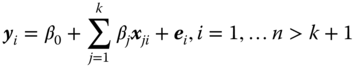
In this section, we use the regression model
with n larger than the number of unknown components of β. The xi may be vectors ![]() , if k = 1 we speak about simple regression, and if k > 1 about multiple regression. For (8.1) the assumptions 1–4 are given above.
, if k = 1 we speak about simple regression, and if k > 1 about multiple regression. For (8.1) the assumptions 1–4 are given above.
8.2.1 Linear and Quasilinear Regression
8.2.1.1 Parameter Estimation
When we know nothing about the distribution of the error terms, we use the least squares method, which gives the same results as the maximum likelihood method for normally distributed y. An estimator ![]() of the regression coefficient β using the least squares method is an estimator where its realisations
of the regression coefficient β using the least squares method is an estimator where its realisations ![]() fulfil
fulfil
This leads to the estimators ((XTX)−1 existing because rank (X) = k + 1 ≤ n)
The variance var(b) of the vector b is
From the Gauss–Markow theorem (Rasch and Schott (2018)), Theorem 4.3) we know that the least squares method gives in linear models linearly unbiased estimators with minimal variance – so‐called best linear unbiased estimators (BLUE).
We write (XTX)−1 = (cij), i, j = 0, 1, … , k and use this later in the testing part.
For those not familiar with matrix notation we can use the following way.
Determine the minimum of

We obtain the minimum by deriving to β and zeroising the derivatives, and checking that the solution gives a minimum. The solution we call ![]() , the least squares estimate and switching to random variables yi gives the least squares estimator
, the least squares estimate and switching to random variables yi gives the least squares estimator ![]() .
.
The components of β in (8.5) are called regression coefficients, the components of (8.3) are the estimated regression coefficients.
We consider the special case of simple linear regression
Zeroising these derivatives gives the so‐called normal equations.
The values of β0 and β1, minimising S = ![]() are denoted by b0 and b1. We obtain the following equations by putting the partial derivatives with respect to β0 and β1 above equal to zero and replacing all yi by the random variable yi. (We check the fact that we really obtain a minimum by showing that the matrix of the second partial derivatives of S is positive definite). When S is a convex function, the solution of the first partial derivatives of S equal to zero gives a minimum.
are denoted by b0 and b1. We obtain the following equations by putting the partial derivatives with respect to β0 and β1 above equal to zero and replacing all yi by the random variable yi. (We check the fact that we really obtain a minimum by showing that the matrix of the second partial derivatives of S is positive definite). When S is a convex function, the solution of the first partial derivatives of S equal to zero gives a minimum.
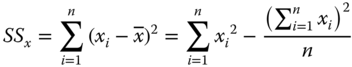
We write with SS the sum of squares and SP the sum of products:
and

and obtain

and
8.2.1.2 Confidence Intervals and Hypotheses Testing
For confidence estimation and hypotheses testing we must assume that the error terms e of the corresponding regression models are independent and normally distributed (N(0, σ2)).We construct confidence intervals for the regression coefficients and confidence, and prediction intervals for the regression line for the simple linear regression only.
If t(f;P) is the P‐quantile of the t‐distribution with f degrees of freedom and CS(f;P) the P‐quantile of the chi‐squared distribution with f degrees of freedom we obtain the following (1−α)100% confidence intervals for βj, j = 0, 1 based on n > 2 data pairs
and σ 2
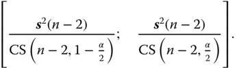
Equation (8.23) is not the best solution, there is a shorter interval obtained by α = α1 + α2 as a sum of positive components α1 and α2 different from α1 = α2 = α/2 and then replacing α/2 by α1 and 1 − α/2 by 1 − α2 in (8.23). The reason for this is the asymmetry of the chi‐squared distribution.
For E(y) = β0 + β1x for any x in the experimental region we need the value of the following quantity Kx:

and then the (1 − α) confidence interval for E(y) = β0 + β1x is:
If we calculate (8.24) for each x‐value in the experimental region, and draw a graph of the realised upper and lower limits, the included region is called a confidence belt.
8.2.2 Intrinsically Non‐Linear Regression
In this section, we give estimates for parameters in such regression functions, which are non‐linear in x and in the parameter vector β.
8.2.2.1 The Asymptotic Distribution of the Least Squares Estimators
For the asymptotic distribution of the least squares estimators, i.e. the distribution of the estimators if the number of observation n tends to infinity, we use results of an important theorem of Jennrich (1969). We need some notation – readers with a less mathematical background may skip the next part.
We assume that the function f(x, β) in Definition 8.2 is twice continuously differentiable with respect to β. For the n regressor values we obtain f(xi, β), i = 1, …, n. We consider the abbreviations:
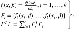
We assume that FTF is positive definite and ![]() is the asymptotic information matrix.
is the asymptotic information matrix.
Jennrich (1969) showed that ![]() is asymptotically
is asymptotically
distributed.
We call
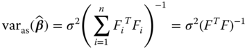
for each n the asymptotic covariance matrix of ![]() (a bit strange but generally in use).
(a bit strange but generally in use).
We estimate ![]() by
by

In ![]() we replace the parameters by their estimators and
we replace the parameters by their estimators and ![]() is given by (8.30).
is given by (8.30).
Based on the estimated asymptotic covariance matrix we can derive test statistics to test the hypothesis that a component βj of β equals βj0 as

and this statistic is asymptotically t‐distributed with n − k degrees of freedom.
Analogous to (8.22) we obtain asymptotic confidence intervals for a component βj as
From now on we write in the special functions below ![]() or
or ![]() .
.
How good the corresponding tests (or confidence intervals) for small n are was investigated by simulation studies, which followed the scheme below:
For the role simulations play in statistics, see Pilz et al. (2018).
For simulations reported for special functions resulting from a research project of Rasch at the University of Rostock during the years 1980 to 1990, see Rasch and Schimke (1983) and Rasch (1990).
The hypothesis Hj0 : βj = βj0 is tested against Hj0 : βj ≠βj0 with the test statistic (8.32). For each of 10 000 runs we added pseudorandom numbers ei from a normal distribution with expectation 0 and variance σ2 to the values of the function f(xi, θ) at n fixed support points inxi [xl, xu]. Then for each i
is a simulated observation. We calculate then from the n simulated observation the least squares estimates ![]() , the estimate
, the estimate ![]() of σ2 and the realisation
of σ2 and the realisation ![]() of the test statistic (8.34). We then calculated 10 000 test statistic tj and counted how often tj fulfilled
of the test statistic (8.34). We then calculated 10 000 test statistic tj and counted how often tj fulfilled
where αnom is the nominal confidence coefficient (risk of the first kind) and αact is the actual confidence coefficient (risk of the first kind) reached by the simulation
respectively (the null hypothesis in the simulation was always correct), divided by 10 000 giving an estimate of αact. Further 10 000 runs to test ![]() with three Δj values have been performed to get information about the power.
with three Δj values have been performed to get information about the power.
We now consider a two‐parametric and four three‐parametric intrinsically non‐linear regression functions important in applications and report the corresponding simulation results, changing the parameter symbols as mentioned above.
8.2.2.2 The Michaelis–Menten Regression
Michaelis–Menten kinetics is one of the best‐known models of enzyme kinetics. It is named after German biochemist Michaelis and Canadian physician Menten. The model takes the form of an equation relating reaction rate y

with the concentration x of a substrate. Michaelis and Menten (1913) published the data of Example 8.5 and an equation of the form
8.2.2.3 Exponential Regression
The model
is an exponential regression model where γ is the non‐linearity parameter. αβγ ≠ 0 implies that no parameter is zero. Brody (1945) used it as a growth function – therefore model (8.42) is sometimes called Brody's model.
The least squares estimates a, b, c of α, β, γ are found by solving the first partial derivatives of y equal to zero and solve the simultaneous equations
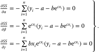
For the solution of these simultaneous equations we check whether there is a minimum. This means that the matrix of the second partial derivatives must have positive eigenvalues.
From Rasch and Schott (2018, Chapter 9) we know that

We will not use this way in this section because R finds the minimum directly, as shown in Problem 8.19
Minimising  gives us the estimates a, b, c of α, β, γ.
8.2.2.4 The Logistic Regression
The model

is the model of a logistic regression where γ is the non‐linearity parameter. αβγ ≠ 0 implies that no parameter is zero. The term logistic regression is not uniquely used – see Chapter 11 for another use of this term.
The first and second derivative to x are

and

At the inflection point (xω, ηω), the numerator of the second derivative has to be zero so that
The second derivative ![]() changes at xω its sign and we really obtain an inflection point.
changes at xω its sign and we really obtain an inflection point.
Now we show that the same curve is described by more than one function. The transition from one function to another is called reparametrisation.
Because ![]() we have
we have

The logistic regression function is written as the three‐parametric hyperbolic tangent‐regression function.
8.2.2.5 The Bertalanffy Function
The regression function fB(x) of the model
is called the Bertalanffy function and was used by Bertalanffy (1929) to describe the growth of the body weight of animals. This function has two inflection points if α and β have different signs and are located at

respectively
8.2.2.6 The Gompertz Function
The regression function fG(x, θ) of the model
is the Gompertz‐Function. In Gompertz (1825) it was used to describe the population growth. The function has an inflection point at

8.2.3 Optimal Experimental Designs
In a model I of regression, we determine the values of the predictor variable in advance. Clearly, we would wish to do this so that a given precision can be reached using a minimal number of observations. In this context, any selection of the x‐values is called an experimental design. The value of the precision requirement is called the optimality criterion, and an experimental design that minimises the criterion for a given sample size is called an optimal experimental design.
Most optimal experimental designs are concerned with estimation criteria. Thus, the xi values are often chosen in such a way that the variance of an estimator is minimised (for a given number of measurements) amongst all possible allocations of xi values for linear or quasilinear regression functions. In the case of an intrinsically non‐linear regression function, the asymptotic variance of an estimator is minimised.
First we have to define the so‐called experimental region (xl, xu) in which measurements can or will be taken. Here xl is the lower bound and xu the upper bound of an interval on the x‐axis.
A big disadvantage of optimal designs is their dependence on the accuracy of the chosen model, they are only certain to be optimal if the assumed model is correct.
8.2.3.1 Simple Linear and Quasilinear Regression
8.2.3.2 Intrinsically Non‐linear Regression
For intrinsically non‐linear regression models, the covariance matrix cannot be used for defining optimal design because it is unknown. We therefore use the asymptotic covariance matrix, but it unfortunately depends on at least one of the unknown parameters. Even if Rasch (1993) could show that the position of the support points often only slightly depends on θ we must check this for each special regression function separately. We therefore can find optimal designs only depending on at least one of the function parameters, we call such designs therefore locally optimal. We denote the part of θ which occurs in the formula of ![]() in (8.33) by θ0 and write θ0 as an argument of the asymptotic covariance matrix as
in (8.33) by θ0 and write θ0 as an argument of the asymptotic covariance matrix as ![]() . At first, some general results are presented and later locally optimal designs for the functions in Section 8.2.3.1 are given.
. At first, some general results are presented and later locally optimal designs for the functions in Section 8.2.3.1 are given.
The asymptotic covariance matrix ![]() can now be written in dependency on θ0 and Vn, m ∈ V (V is the set of all admissible designs) as
can now be written in dependency on θ0 and Vn, m ∈ V (V is the set of all admissible designs) as
and ![]() is called a locally D‐, G‐ or C‐optimal m‐point design at θ = θ0, if
is called a locally D‐, G‐ or C‐optimal m‐point design at θ = θ0, if
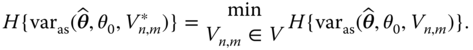
Here H means any of the criteria D, G or C.
If Vm is the set of concrete m‐point designs, then ![]() is called concrete locally H‐optimal m‐point design, if
is called concrete locally H‐optimal m‐point design, if

For some regression functions and optimality criteria analytical solutions in closed form of the problems could be found. Otherwise, search methods are applied.
The first analytical solution we find in Box and Lucas 1959 in Theorem 8.1.
8.2.3.3 The Michaelis‐Menten Regression
The locally D‐optimum design of the function ![]() in [a,b] is for even n = 2t given by (Ermakov and Zigljavski 1987):
in [a,b] is for even n = 2t given by (Ermakov and Zigljavski 1987):

For odd n = 2 t + 1 we have two locally D‐optimum designs namely  and
and  respectively.
In the interval [0, 1440], which was used in Table 8.6 we had n = 10 and by this t = 5. With the parameter estimated the locally D‐optimum design is given as

with the criterium value 6.445. The original design of Michaelis and Menten in the form
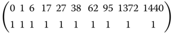
has the criterion value 16.48.
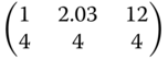
Rasch (2008) found by search procedures the locally C1‐optimal design  and the locally C2‐optimal design
 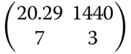 .
.
8.2.3.4 Exponential Regression
By constructing locally optimal designs in the class of m‐point designs (m ≥ 3) only such optimal designs have been found which are three‐point designs as derived by Box and Lucas (1959) for n = 3.
In Table 8.11 we list for rounded estimated parameter values found in the example of Problem 8.19 (oil palm data) and smaller and larger values of these parameters the locally D‐ and Ci(i = 1, 2, 3)‐optimal designs.
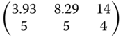
Table 8.11 Locally optimal designs for the exponential regression.
| Criterion | (α,β,γ) = (14,−18, −0.2) | (α,β,γ) = (16.5, −16.7, −0.14) | (α,β,γ) = (18, −17, −0.097) |
| D |  |
 |
 |
| C1 |  |
 |
 |
| C2 | 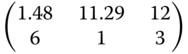 |
 |
 |
| C3 |  |
 |
 |
We compare the criterion value 0.00015381σ6 of the D‐optimal design  with the criterion value of the design
  used in the experiment, which is 0.0004782σ6.
8.2.3.5 The Logistic Regression
By constructing locally optimal designs in the class of m‐point designs (m ≥ 3) only three‐point designs have been found.
In Table 8.12 we list for rounded estimated parameter values found in the example of Problem 8.23 (hemp data) and smaller and larger values of these parameters the locally D‐ and Ci (i = 1, 2, 3)‐optimal designs.
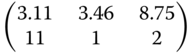
Table 8.12 Locally optimal designs for the logistic regression.
| Criterion | (α,β,γ) = (123,16, −0.5) | (α,β,γ) = (126,20, −0.46) | ((α,β,γ) = (130,23, −0.42) |
| D |  |
 |
 |
| Cα |  |
 |
 |
| Cβ |  |
 |
 |
| Cγ | 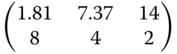 |
 |
 |
8.2.3.6 The Bertalanffy Function
By constructing locally optimal designs in the class of m‐point designs (m ≥ 3) only three‐point designs have been found.
In Table 8.13 we list for rounded estimated parameter values found in the example of Problem 8.28 (oil palm data) and smaller and larger values of these parameters the locally D‐ and Ci (i = 1, 2, 3)‐optimal designs.
Table 8.13 Locally optimal designs for the Bertalanffy regression.
| Criterion | (α,β,γ) = (2.35, −1.63, −0.31) | (α,β,γ) = (2.44, −1.43, −0.24) | (α,β,γ) = (2.54, −1.23, −0.17) |
| D |  |
 |
 |
| C1 |  |
 |
 |
| C2 |  |
 |
 |
| C3 |  |
 |
 |
8.2.3.7 The Gompertz Function
By constructing locally optimal designs in the class of m‐point designs (m ≥ 3) only three‐point designs have been found.
In Table 8.14 we list for rounded estimated parameter values found in the example of Problem 8.31 and smaller and larger values of these parameters the locally D‐ and Ci (i = 1, 2, 3)‐optimal designs.
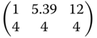
Table 8.14 Locally optimal designs for the Gompertz regression.
| Criterion | (β,γ) = (−17,−0.14) | (β,γ) = (−19,−0.2) | (β,γ) = (−14,−0.08) |
| D |  |
 |
 |
| Cα |  |
 |
 |
| Cβ |  |
 |
 |
| Cγ |  |
 |
 |
8.3 Models with Random Regressors
We consider mainly the linear or quasilinear case for model II of the regression analysis where not only the regressand but also the regressor is a random variable. As mentioned at the top of this chapter we use the regression model
where the following assumptions must be fulfilled:
- The error terms ei are random variables with expectation zero.
- The variance of the error terms ei is equal for all observations.
- For hypotheses testing and confidence estimation we assume that the ei are N(0, σ2) distributed.
- The error terms ei are independent of the regressor variables xi.
 .
.
Intrinsically non‐linear regression models with random regressors are more the exception than the rule and play a minor role. An exception is the relative growth of a part of a body to the whole body or another part, we speak about allometry and consider this in Section 8.3.2.
8.3.1 The Simple Linear Case
The model
with the additional assumptions (1) to (5) is called a model II of the (if k > 1, multiple) linear regression. Correlation coefficients are defined, as long as (8.79) holds and the distribution has finite second moments.
We first discuss the case with k = 1 and
is the simple linear model II. Of course, we may interchange regressor and regressand and consider the model
Instead of discussing both models we simply rename the two variables and come back to (8.80).
The two‐dimensional density distribution of  may have existing second moments so that

In model I we had E(yi) = β0 + β1xi but now from (8.81) we see that E(yi) = β0 + β1μx ∀ i and does not depend on the regressor variable. The estimator of (8.81) is

We consider the conditional expectation (i.e. the expectation of the conditional distribution of y for given x = x).
and the right‐hand side of (8.82) equals (8.6) for model I.
Because the parameter estimation in model II is done for this conditional expectation (8.82) the formulae for the estimates are identical for both models. This is a reason why program packages like IBM SPSS‐Statistics and SAS in regression analysis do not ask which model is assumed for the data as in the analysis of variance.
The estimators are

and
Graybill (1961) showed with lemma 10.1 that  . Further
Even if the  are (independently) normally distributed,
  is not normally distributed.
The ratio
is called the correlation coefficient between x and y.
By replacing ![]() and
and ![]() by their unbiased estimators
by their unbiased estimators ![]() and
and ![]() we get the (biased) estimator
we get the (biased) estimator
of the correlation coefficient.
To test the hypothesis H0: ρ ≤ ρ0 against the alternative hypothesis HA: ρ > ρ0 (respectively H0: ρ ≥ ρ0 against HA: ρ < ρ0). we replace r by the modified Fisher transform
which is approximately normally distributed even if n is rather small. Cramér (1946) proved that for n = 10 the approximation is actually sufficient as long as −0.8 ≤ ρ ≤ 0.8. The expectation E of z, being a function ζ of ρ, amounts to

The statistic z in (8.87) can be used to test the hypothesis H0: ρ ≤ ρ0 against the alternative hypothesis HA: ρ > ρ0 (respectively H0: ρ ≥ ρ0 against HA: ρ < ρ0). H0: ρ ≤ ρ0 is rejected with a first kind risk α, if z ≥ ζ(ρ0)+ z1‐α ·![]() (respectively for H0: ρ ≥ ρ0. if z ≥ ζ(ρ0) – z1‐α ·
(respectively for H0: ρ ≥ ρ0. if z ≥ ζ(ρ0) – z1‐α ·![]() ); z1‐α is the (1 − α)‐quantile of the standard normal distribution).
); z1‐α is the (1 − α)‐quantile of the standard normal distribution).
We use a sequential triangular test (Whitehead 1992; Schneider 1992). We split the sequence of data pairs into sub‐samples of length, say k > 3 each. For each sub‐sample j (j = 1, 2, … m) we calculate a statistic of which distribution is only a function of ρ and k.
A triangular test must be based on a statistic with expectation 0, given the null‐hypothesis, therefore we transform z into a realisation of a standardised variable

which has the expectation 0 if the null‐hypothesis is true.
The parameter

is used as a test parameter. For ρ = ρ0 the parameter θ is zero (as demanded). For ρ = ρ1 we obtain:
The difference δ = ρ1 − ρ0 is the practical relevant difference which should be detected with power 1 − β.
From each sub‐sample j we now calculate the sample correlation coefficient rj as well as its transformed values ![]() (j = 1, 2, …, m).
(j = 1, 2, …, m).
Now by ![]() and Vm = m the sequential path is defined by points (Vm, Zm) for m = 1, 2, … up to the maximum of V below or exactly at the point where a decision can be made. The continuation region is a triangle whose three sides depend on α, β, and θ1via
and Vm = m the sequential path is defined by points (Vm, Zm) for m = 1, 2, … up to the maximum of V below or exactly at the point where a decision can be made. The continuation region is a triangle whose three sides depend on α, β, and θ1via

and

with the percentiles zP of the standard normal distribution. That is, one side of the looked‐for triangle lies between –a and a on the ordinate of the (V, Z) plane (V = 0). The two other borderlines are defined by the lines L1: Z = a + cV and L2: Z = −a + 3cV, which intersect at
The maximum sample size is of course k·Vmax. The decision rule now is: Continue sampling as long as −a + 3cVm < Zm < a + cVm if θ1 > 0 or −a + 3cVm > Zm > a + cVm if θ1 < 0. Given θ1 > 0, accept HA in case that Zm reaches or exceeds L1 and accept H0 in case that Zm reaches or underruns L2, Given θ1 < 0, accept HA in the case Zm reaches or underruns L1 and accept H0 in the case Zm reaches or exceeds L2. If the point ![]() is reached, HA to be accepted.
is reached, HA to be accepted.
What values must be chosen for k? The answer was found by a simulation experiment in Rasch et al. (2018) where
- (a) the optimal size of subsamples (kopt), where the actual type‐I‐risk (αact) is below but as close as possible to the nominal type‐I‐risk (αnom) was determined and
- (b) the optimal nominal type‐II‐risk (βopt), where the corresponding actual type‐II‐risk (βact) is below but as close as possible to the nominal type‐II‐risk (βnom) was determined.
Starting from k = 4, the size of the subsample was systematically increased with an increment of 1 for each parameter combination until the actual type‐I‐risk (αact) fell below the nominal type‐I‐risk (αnom). This optimal size of subsample (kopt) was found in the next step to determine the optimal nominal type‐II‐risk (βopt). That is, the nominal type‐II‐risk (βnom) was systematically increased with an increment of 0.005 until the actual type‐II‐risk (βact) fell below the nominal type‐II‐risk (αnom).
Paths (Z, V) were generated by bivariate normally distributed random numbers x and y with means μx = μy = 0, variances ![]() =
= ![]() = 1, and a correlation coefficient σxy = ρ.
= 1, and a correlation coefficient σxy = ρ.
Using the seqtest package version 0.1‐0 (Yanagida 2016) simulations can be performed for any αnom, βnom, and δ =ρ1 − ρ0. We present here results for nominal risks αnom = 0.05 and 0.01, βnom = 0.1 and 0.2, values of ρ0 ranging 0.1–0.9 with an increment of 0.1, and δ =ρ1 − ρ0= 0.05, 0.10, 0.15, and 0.20.
For each parameter, combination 1 000 000 runs (paths) were generated. As criteria, we calculated:
- (a) the relative frequency of wrongly accepting H1, given ρ = ρ0, which is an estimate of the actual type‐I‐risk (αact),
- (b) the relative frequency of keeping H0, given ρ = ρ1 which is an estimate of the actual type‐II‐risk (βact),
- (c) the average number of sample pairs (x, y), i.e. average sample number (ASN), is the mean (Table 8.15).
Table 8.15 Optimal size of sub‐samples (k) and optimal nominal type‐II‐risk (βopt) values for αnom = 0.05.
| Given values of the test problem | Optimal values | ||||
| ρ0 | ρ1 | β | kopt | βopt | ASN | ρ1 |
| 0.2 | 0.25 | 0.1 | 78 | 0.125 | 1909 |
| 0.2 | 65 | 0.235 | 1532 | ||
| 0.30 | 0.1 | 33 | 0.130 | 491 | |
| 0.2 | 27 | 0.245 | 396 | ||
| 0.35 | 0.1 | 20 | 0.135 | 224 | |
| 0.2 | 16 | 0.250 | 183 | ||
| 0.40 | 0.1 | 14 | 0.140 | 129 | |
| 0.2 | 12 | 0.260 | 106 | ||
| 0.3 | 0.35 | 0.1 | 76 | 0.125 | 1710 |
| 0.2 | 79 | 0.240 | 1364 | ||
| 0.40 | 0.1 | 38 | 0.135 | 428 | |
| 0.2 | 32 | 0.250 | 348 | ||
| 0.45 | 0.1 | 23 | 0.140 | 193 | |
| 0.2 | 19 | 0.255 | 158 | ||
| 0.50 | 0.1 | 16 | 0.150 | 109 | |
| 0.2 | 13 | 0.270 | 90 | ||
| 0.5 | 0.55 | 0.1 | 102 | 0.140 | 1122 |
| 0.2 | 83 | 0.245 | 916 | ||
| 0.60 | 0.1 | 41 | 0.145 | 278 | |
| 0.2 | 33 | 0.265 | 224 | ||
| 0.65 | 0.1 | 23 | 0.155 | 120 | |
| 0.2 | 19 | 0.275 | 98 | ||
| 0.70 | 0.1 | 16 | 0.165 | 66 | |
| 0.2 | 13 | 0.285 | 54 | ||
| 0.7 | 0.75 | 0.1 | 73 | 0.145 | 503 |
| 0.2 | 61 | 0.265 | 403 | ||
| 0.80 | 0.1 | 28 | 0.165 | 115 | |
| 0.2 | 23 | 0.285 | 94 | ||
| 0.85 | 0.1 | 15 | 0.180 | 46 | |
8.3.2 The Multiple Linear Case and the Quasilinear Case
In the case k = 2 random variable (x1, x2, x3) is assumed to be three‐dimensional normally distributed with existing second moments. Any of these three random variables may be use as regressand y in the regression model and the other renamed as x1, x2
as special case of (8.79) [with assumptions (1) to (5)].
Unbiased estimators of β0, β1, β2 can be received analogous to (8.83) and (8.84).
The three conditional two‐dimensional distributions are two‐dimensional distributions with correlation coefficients

Here ρij,ρik and ρjk are the correlation coefficients of the three two‐dimensional marginal distributions of (xi,xj,xk). It can easily be shown that these marginal distributions are two‐dimensional normal distributions if (x1,x2,x3) is normally distributed.
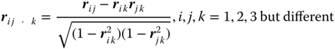
The correlation coefficient (8.89) of the conditional two‐dimensional normal distribution of (xi,xj) for given xk, i, j, k = 1, 2, 3 but different is called the partial correlation coefficient between (xi,xj) after fixing xk at xk.
We obtain estimators ri j · k for partial correlation coefficients by replacing the simple correlation coefficients in (8.87) by their estimators and obtain the biased estimators
For the general parameter estimation, we use the formulae in Section 8.2
8.3.2.1 Hypotheses Testing ‐ General
Bartlett (1933) showed that all the tests in 8.2.1.2 could be applied also for model II, but the power of the tests differ between both models.
8.3.2.2 Confidence Estimation
An approximate (1 − α) 100%‐confidence interval for ϱ is

with the ![]() ‐quantile
‐quantile ![]() of the standard normal distribution
of the standard normal distribution ![]() .
.
To interpret the value of ϱ (and also of r), we again consider the regression function f(x) = E(y|x) = β0 + β1x.
ϱ2 can now be explained as a measure of the proportion of the variance of y, explainable by the regression on x. The conditional variance of y is
and

is the proportion of the variance of y, not explainable by the regression on x, and by this the statement above follows. We call ϱ2 = B measure of determination.
To construct confidence intervals for β0 and β1 or to test hypotheses about these parameters seems to be difficult but the methods for model I can also be applied for model II. We demonstrate this for the example of the confidence interval for β0. The argumentation for confidence intervals for other parameters and for the statistical tests is analogous.
The probability statement

leading to the confidence interval (8.58) for j = 0 is true, if for fixed values x1, … , xn samples of y values are selected repeatedly. Using the frequency interpretation, β0 is covered in about (1 − α) 100% of the cases by the interval (8.58). This statement is valid for each arbitrary n‐tuple xi l, … , xin, also for an n‐tuple xi l, … , xin, randomly selected from the distribution because (8.58) is independent of x1, … , xn, if the conditional distribution of the yj is normal. However, this is the case, because (y, x1, … , xk) was assumed to be normally distributed. By this the construction of confidence intervals and testing of hypotheses can be done by the methods and formulae given above. However, the expected width of the confidence intervals and the power function of the tests differ for both models.
That ![]() is really a confidence interval with a confidence coefficient 1 − α also for model II, can of course be proven exactly, using a theorem of Bartlett (1933) by which
is really a confidence interval with a confidence coefficient 1 − α also for model II, can of course be proven exactly, using a theorem of Bartlett (1933) by which

is t(n − 2)‐distributed.
8.3.3 The Allometric Model
In model II we discuss only one intrinsically non‐linear model, the allometric model
first used by Snell (1892) to describe the dependency between body mass and brain mass.
The allometric model is mainly used to describe relative growth of one part of a growing individual (plant or animal) to the total mass or the mass of another part see Huxley (1972). Nowadays this model is also used in technical applications.
8.3.4 Experimental Designs
The experimental design for model II of the regression analysis differs fundamentally from that of model I. Because x in model II is a random variable, the problem of the optimal choice of x does not occur. Experimental design in model II means only the optimal choice of n in dependency of given precision requirements. A systematic description about that is given in Rasch et al. (2008). We repeat this in the following.
At first we restrict in (8.59) on k = 1, and consider the more general model of the regression within of ![]() groups with the same slope β1
groups with the same slope β1
We estimate β1 for a > 1 not by 8.9, but by

with ![]() for each of the a groups as defined in Example 8.1.
for each of the a groups as defined in Example 8.1.
If we look for a minimal  so that
 ![]() we find in Bock (1998)
we find in Bock (1998)

If k = 1 for the expectation E(y|x) = β0 + β1x (1 − α)− confidence interval should be given so that the expectation of the square of the half width of the interval does not exceed δ, then

must be chosen.
References
- Atkinson, A.C. and Hunter, W.G. (1968). The design of experiments for parameter estimations. Technometrics 10: 271–289.
- Barath, C.S., Rasch, D., and Szabo, T. (1996). Összefügges a kiserlet pontossaga es az ismetlesek szama kozött. Allatenyesztes es takarmanyozas 45: 359–371.
- Bartlett, M.S. (1933). On the theory of statistical regression. Proc. Royal Soc. Edinburgh 53: 260–283.
- Bertalanffy, L. von (1929). Vorschlag zweier sehr allgemeiner biologischer Gesetze. Biol. Zbl. 49: 83–111.
- Bock, J. (1998). Bestimmung des Stichprobenumfanges für biologische Experimente und kontrollierte klinische Studien. München Wien: R. Oldenbourg Verlag.
- Box, G.E.P. and Lucas, H.L. (1959). Design of experiments in nonlinear statistics. Biometrics 46: 77–96.
- Brody, S. (1945). Bioenergetics and Growth. N.Y: Rheinhold Pub. Corp.
- Cramér, H. (1946). Mathematical Methods of Statistics. Princeton: Princeton University Press.
- Ermakov, S.M. and Zigljavski, A.A. (1987). Математическая теория оптималных экспериметов (Mathematical Theory of Optimal Experiments). Moskwa: Nauka.
- Galton, F. (1885). Opening address as President of the Anthropology Section of the British Association for the Advancement of Science, September 10th, 1885, at Aberdeen. Nature 32: 507–510.
- Gompertz, B. (1825). On the nature of the function expressive of the law of human mortality, and on a new method determining the value of life contingencies. Phil. Trans. Roy. Soc. (B), London 513–585.
- Graybill, A.F. (1961). An Introduction to Linear Statistical Models. New York: Mc Graw Holl.
- Huxley, J.S. (1972). Problems of Relative Growth, 2e. New York: Dover.
- Jennrich, R.J. (1969). Asymptotic properties of nonlinear least squares estimation. Ann. Math. Stat. 40: 633–643.
- Michaelis, L. and Menten, M.L. (1913). Die Kinetik der Invertinwirkung. Biochem. Z. 49: 333–369.
- Pilz, J., Rasch, D., Melas, V.B., and Moder, K. (eds.) (2018). Statistics and Simulation: IWS 8, Vienna, Austria, September 2015, Springer Proceedings in Mathematics & Statistics, vol. 231. Heidelberg: Springer.
- Pukelsheim, F. (1993). Optimal Design of Experiments. New York: Wiley.
- Rasch, D. (1968). Elementare Einführung in die Mathematische Statistik. Berlin: VEB Deutscher Verlag der Wissenschaften.
- Rasch, D. (1990). Optimum experimental design in nonlinear regression. Commun. Stat. Theory and Methods 19: 4789–4806.
- Rasch, D. (1993). The robustness against parameter variation of exact locally optimum experimental designs in growth models ‐ a case study. In: Techn. Note 93‐3. Department of Mathematics, Wageningen Agricultural University.
- Rasch, D. (2008) Versuchsplanung in der nichtlinearen Regression ‐ Michaelis‐Menten gestern und heute. Vortrag an der Boku Wien, Mai 2008.
- Rasch, D. and Schimke, E. (1983). Distribution of estimators in exponential regression – a simulation study. Skand. J. Stat. 10: 293–300.
- Rasch, D. and Schott, D. (2018). Mathematical Statistics. Oxford: Wiley.
- Rasch, D., Herrendörfer, G., Bock, J. et al. (eds.) (2008). Verfahrensbibliothek Versuchsplanung und ‐ auswertung, 2. verbesserte Auflage in einem Band mit CD. München Wien: R. Oldenbourg Verlag.
- Rasch, D., Yanagida, T., Kubinger, K.D., and Schneider, B. (2018). Determination of the optimal size of subsamples for testing a correlation coefficient by a sequential triangular test. In: Statistics and Simulation: IWS 8, Vienna, Austria, September 2015, Springer Proceedings in Mathematics & Statistics, vol. 231 (ed. J. Pilz, D. Rasch, V.B. Melas and K. Moder).
- Schlettwein, K. (1987). Beiträge zur Analyse von vier speziellen Wachstumsfunktionen. Rostock: Dipl.Arbeit, Sektion Mathematik, Univ.
- Schneider, B. (1992). An interactive computer program for design and monitoring of sequential clinical trials. In Proceedings of the XVIth international biometric conference (pp. 237–250), Hamilton, New Zealand.
- Snell, O. (1892). Die Abhängigkeit des Hirngewichts von dem Körpergewicht und den geistigen Fähigkeiten. Arch. Psychiatr. 23: 436–446.
- Steger, H. and Püschel, F. (1960). Der Einfluß der Feuchtigkeit auf die Haltbarkeit des Carotins in künstlich getrocknetem Grünfutter. Die Deutsche Landwirtschaft 11: 301–303.
- Whitehead, J. (1992). The Design and Analysis of Sequential Clinical Trials, 2e. Chichester: Ellis Horwood.
- Yanagida, T. (2016). seqtest: Sequential triangular test, R package version 0.1‐0. http://CRAN.R‐project.org/package=seqtest.
- Yule, G.U. (1897). On the theory of correlation. J. R. Stat. Soc. 60 (4): 812–854, Blackwell Publishing.