
Chapter 8. Drawing Elevations, Sections, and Details
• Correctly use the following commands and settings:
Edit Hatch
HATCH
MIRROR
Multileader
Multileader Style
OTRACK
Point Filters
STRETCH
UCS
UCS Icon
Introduction
The AutoCAD program makes it possible to produce clear, accurate, and impressive drawings of elevations, sections, and details. Many of the commands you have already learned are used in this chapter, along with some new commands.
EXERCISE 8-1 Tenant Space: Elevation of Conference Room Cabinets
In Exercise 8-1, an elevation of the south wall of the tenant space conference room is drawn. The south wall of the tenant space conference room has built-in cabinets that include a refrigerator and a sink. When you have completed Exercise 8-1, your drawing will look similar to Figure 8-1.

Figure 8-1 Exercise 8-1: Tenant space, elevation of conference room cabinets (scale: 1/2′ = 1′-0″)
Step 1. Use your workspace to make the following settings:
1. Use Save As... to save the drawing on the hard drive with the name CH8-EXERCISE1.
2. Set drawing units: Architectural
3. Set drawing limits: 25′,24′
5. Set grid: 12″
6. Set snap: 6″
7. Create the following layers:

8. Set layer a-elev-lwt1 current.
9. Use Zoom-All to view the limits of the drawing.
UCS
While you were drawing with AutoCAD in previous chapters the UCS icon was located in the lower left corner of your drawings. A coordinate system is simply the X, Y, and Z coordinates used in your drawings. For 2D drawings, only the X and Y coordinates are meaningful. The Z coordinate is used for a three-dimensional model.
Notice that the 2D UCS icon (Figure 8-2) has a W on it. The W stands for world coordinate system. This is the AutoCAD fixed coordinate system, which is common to all AutoCAD drawings. Your version of AutoCAD uses the 3D icon by default, showing only X- and Y-axes, so the W is not visible.

The UCS command is used to set up a new user coordinate system. When UCS is typed from the command prompt, the prompt is Specify origin of UCS or [Face NAmed OBject Previous View World X Y Z ZAxis] <World>:. The Z coordinate is described and used extensively in the chapters that cover 3D modeling. The UCS command options that apply to two dimensions are listed next.

user coordinate system: A user-defined variation of the world coordinate system. Variations in the coordinate system range from moving the default drawing origin (0,0,0) to another location to changing orientations for the X-, Y-, and Z-axes. It is possible to rotate the world coordinate system on any axis to make a UCS with a different two-dimensional XY plane.
Specify origin of UCS: Allows you to create a new UCS by selecting a new origin and a new X-axis. If you select a single point, the origin of the current UCS moves without changing the orientation of the X- and Y-axes.
NAmed: When this option is entered, the prompt Enter an option [Restore Save Delete?] appears. It allows you to restore, save, delete, and list named user coordinate systems.
OBject: Allows you to define a new UCS by pointing to a drawing object such as an arc, point, circle, or line.
Previous: Makes the previous UCS current.
World: The AutoCAD fixed coordinate system, which is common to all AutoCAD drawings. In most cases you will want to return to the world coordinate system before plotting any drawing.
Step 2. Use the UCS command to change the origin of the current UCS, as described next:
Prompt |
Response |
Type a command: |
Type UCS <Enter> |
Specify origin of UCS or [Face NAmed OBject Previous View World X Y Z ZAxis] <World> |
Type: 8′,12′ <Enter> |
Specify point on X-axis or <Accept>: |
<Enter> |
Note
You can change the UCS so you can move 0,0 to any point on your drawing to make it more convenient to locate points.
The origin for the current user coordinate system is now 8′ in the X direction and 12′ in the Y direction. The UCS icon may not have moved from where 0,0 was originally located. The UCS Icon command, described next, is used to control the orientation and visibility of the UCS icon.
UCS Icon
There are two model space UCS icons that you can choose to use: one for 2D drawings and one for 3D drawings. The default is the 3D icon, which you will probably use for both 2D and 3D. The UCS Icon command is used to control the visibility and orientation of the UCS icon (Figure 8-2). The UCS icon appears as lines (most often located in the lower left corner of an AutoCAD drawing) that show the orientation of the X-, Y-, and Z-axes of the current UCS. It appears as a triangle in paper space. The UCS Icon command options are ON OFF All Noorigin ORigin Properties:. The UCS Icon command options follow.
ON: Allows you to turn on the UCS icon if it is not visible.
OFF: Allows you to turn off the UCS icon when it gets in the way. This has nothing to do with the UCS location—only the visibility of the UCS icon.
All: Allows you to apply changes to the UCS icon in all active viewports. (The Viewports command, which allows you to create multiple viewports, is described in Chapter 12.)
Noorigin: When Noorigin is current, the UCS icon is displayed at the lower left corner of the screen.
ORigin: Forces the UCS icon to be displayed at the origin of the current UCS. For example, when USC Icon - Origin is clicked, the new UCS that you just created will appear in its correct position. If the origin of the UCS is off the screen, the icon is still displayed in the lower left corner of the screen.
Properties: When Properties is selected, the UCS Icon dialog box apppears (Figure 8-3). This box allows you to select the 2D or 3D model space icon and to change the size and color of model space and paper space (Layout tab) icons.

Note
The Coordinates panel is hidden in the Ribbon View tab by default. Right-click on the View tab to show the Coordinates panel.
Step 3. If the UCS icon did not move, use the UCS Icon command to force the UCS icon to be displayed at the origin of the new, current UCS, as described next:

Prompt |
Response |
Type a command: |
Type UCSICON <Enter> |
Enter an option [ON OFF All Noorigin ORigin Selectable Properties] <ON>: |
Type OR <Enter> (the UCS icon moves to the 8′,12′ coordinate location) |
Draw the Upper Cabinets
Step 4. Using absolute coordinates, draw a rectangle forming the first upper cabinet door. Start the drawing at 2, 2 (two inches above and two inches to the right of the new UCS), Figure 8-4, as described next:
Response |
|
Type a command: |
Rectangle (or type REC <Enter>) |
Specify first corner point or [Chamfer Elevation Fillet Thickness Width]: |
Type 2,2 <Enter> |
Specify other corner point or [Area Dimensions Rotation]: |
Type 19,44 <Enter> |

Step 5. Use Polyline to draw the door hardware using absolute coordinates (Figure 8-4), as described next:
Prompt |
Response |
Type a command: |
Polyline (or type PL <Enter>) |
Specify start point: |
Type 16,4 <Enter> |
Specify next point or [Arc Halfwidth Length Undo Width]: |
Type W <Enter> |
Specify starting width <0′-0″>: |
Type 1/4 <Enter> |
Specify ending width <0′-0 1/4″>: |
<Enter> |
Specify next point or [Arc Halfwidth Length Undo Width]: |
Type 16,9 <Enter> |
Specify next point or [Arc Close Halfwidth Length Undo Width]: |
<Enter> |
Step 6. Set layer a-elev-hdln current and draw the dashed lines of the door using absolute coordinates (Figure 8-4), as described next:
Prompt |
Response |
Type a command: |
Line (or type L <Enter>) |
Specify first point: |
Type 19,3′8 <Enter> |
Specify next point or [Undo]: |
Type 2,23 <Enter> |
Specify next point or [Undo]: |
Type 19,2 <Enter> |
Specify next point or [Close Undo]: |
<Enter> |
Step 7. Change the linetype scale of the Hidden linetype to make it appear as dashes, change the linetype to Hidden2, or both. A large linetype scale such as 12 is needed. (Type LTSCALE <Enter>, then type 12 <Enter>.)
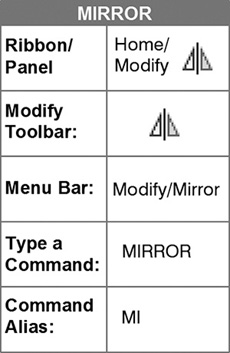
Mirror
The MIRROR command allows you to mirror about an axis any entity or group of entities. The axis can be at any angle.
Step 8. Draw the second upper cabinet door, using the MIRROR command to copy the cabinet door just drawn (Figure 8-5), as described next:
Prompt |
Response |
Type a command: |
Mirror (or type MI <Enter>) |
Select objects: |
P1→ |
Specify opposite corner: |
P2→ |
Select objects: |
<Enter> |
Specify first point of mirror line: |
P3→ (with ORTHO and OSNAP-INTERSECTION on) |
Specify second point of mirror line: |
P4→ |
Erase source objects? [Yes No] <N>: |
<Enter> (to complete command) |

Note
If you want to mirror a part of a drawing containing text but do not want the text to be a mirror image, change the MIRRTEXT system variable setting to 0. This allows you to mirror the part and leave the text “right reading.” When MIRRTEXT is set to 1, the text is given a mirror image. To change this setting, type MIRRTEXT <Enter>, then type 0 <Enter>.
Step 9. Set layer a-elev-lwt1 current. Using relative coordinates, draw a rectangle forming the outside of the upper cabinet. Start the rectangle at the 0,0 location of the new UCS (Figure 8-6), as described next:
Prompt |
Response |
Type a command: |
Rectangle (or type REC <Enter>) |
Specify first corner point or [Chamfer Elevation Fillet Thickness Width]: |
Type 0,0 <Enter> |
Specify other corner point or [Area Dimensions Rotation]: |
Type @9′,3′10 <Enter> |

Step 10. Copy the first two upper cabinet doors 2′11″ and 5′10″ to the right (Figure 8-6) as described next:
Prompt |
Response |
Type a command: |
Copy (or type CP <Enter>) |
Select objects: |
Use a window to select the first two upper cabinet doors |
Select objects: |
<Enter> |
Specify base point or [Displacement mOde] <Displacement>: |
Click any point |
Specify second point or [Array] <use first point as displacement>: |
With ORTHO on, move your mouse to the right and type 2′11 <Enter> |
Specify second point or [Array Exit Undo] <Exit>: |
Move the mouse to the right and type 5′10 <Enter> |
Specify second point or [Exit Undo] <Exit>: |
<Enter> |
Draw the Lower Cabinets
Step 11. Use the MIRROR command to draw the first lower cabinet door (Figure 8-7), as described next:
Response |
|
Type a command: |
Mirror (or type MI <Enter>) |
Select objects: |
P2→ (left to right) |
Specify opposite corner: |
P1→ |
Select objects: |
<Enter> |
Specify first point of mirror line: |
P3→ (with ORTHO and SNAP on; the lower cabinets will be moved to the accurate location later) |
Specify second point of mirror line: |
P4→ |
Erase source objects? [Yes No] <N>: |
<Enter> (the lower cabinet is now too high and too narrow) |

Stretch
The STRETCH command can be used to stretch entities to make them longer or shorter. It can also be used to move entities that have other lines attached to them without removing the attached lines (described later in this exercise). STRETCH requires you to use a crossing window to select objects. As with many other Modify commands, you may select objects initially, then remove or add objects to the selection set before you perform the stretch function.

Step 12. Use the STRETCH command to change the height of the first lower cabinet door just drawn (Figure 8-8), as described next:

Prompt |
Response |
Type a command: |
Stretch (or type S <Enter>) |
Select objects to stretch by crossing-window or crossing-polygon... Select objects: |
P1→ |
Specify opposite corner: |
P2→ |
Select objects: |
<Enter> |
P3→ (any point) |
|
Specify second point or <use first point as displacement>: |
Type @9<270 <Enter> (or with ORTHO on move your mouse down and type 9 <Enter>) (the upper door height, 3′6″, minus the lower door height, 2′, divided by 2; take half off the top of the door and half off the bottom) |
Type a command: |
Stretch (or press <Enter>) |
Select objects to stretch by crossing-window or crossing-polygon... Select objects: |
P4→ |
Specify opposite corner: |
P5→ |
Select objects: |
<Enter> |
Specify base point or [Displacement] <Displacement>: |
P3→ (any point) |
Specify second point or <use first point as displacement>: |
Type @9<90 <Enter> (or move your mouse up and type 9 <Enter>). The lower cabinet door should now be 18″ shorter than the upper cabinet door from which it was mirrored (3′6″ minus 18″ equals 2′, the cabinet door height) |
Step 13. Use the STRETCH command to change the width of the first lower cabinet door (Figure 8-9), as described next:

Prompt |
Response |
Type a command: |
Stretch |
Select objects to stretch by crossing-window or crossing-polygon... Select objects: |
P1→ |
Specify opposite corner: |
P2→ |
Select objects: |
<Enter> |
P3→ (any point) |
|
Specify second point or <use first point as displacement>: |
Type @1-1/2<0 <Enter> (or move the mouse to the right and type 1-1/2 <Enter>) (the upper door width, 1′5″, plus 1-1/2″, equals the lower door width, 1′6-1/2″) |
Step 14. Save the current UCS used to draw the upper cabinets, as described next:
Prompt |
Response |
Type a command: |
Type UCS <Enter> |
Specify origin of UCS or [Face NAmed OBject Previous View World X Y Z ZAxis] <World>: |
Type S <Enter> |
Enter name to save current UCS or [?]: |
Type UPPER <Enter> |
Step 15. Create a new UCS origin for drawing the lower cabinets by moving the existing UCS origin –4′2-1/2″ in the Y direction, as described next.
Prompt |
Response |
Type a command: |
<Enter> (repeat UCS) |
Specify origin of UCS or [Face NAmed OBject Previous View World X Y Z ZAxis] <World>: |
Type O <Enter> |
Specify new origin point <0,0,0>: |
Type 0,-4′2-1/2 <Enter> (be sure to include the minus) |
Step 16. Move the lower cabinet door to a point 2″ above and 2″ to the right of the origin of the current UCS (Figure 8-10), as described next:
Prompt |
Response |
Type a command: |
Move (or type M <Enter>) |
Select objects: |
P1→ (Figure 8-10) |
P2→ |
|
Select objects: |
<Enter> |
Specify base point or [Displacement] <Displacement>: |
Osnap-Intersection |
of |
P3→ |
Specify second point or <use firstpoint as displacement>: |
Type 2,2 <Enter> |

Figure 8-10 Move the lower cabinet door to a point 2″ above and 2″ to the right of the origin of the current UCS
Step 17. Using relative coordinates, draw a rectangle forming the drawer above the lower cabinet door (Figure 8-11), as described next:
Prompt |
Response |
Type a command: |
Rectangle (or type REC <Enter>) |
Specify first corner point or [Chamfer Elevation Fillet Thickness Width]: |
Type FRO <Enter> Osnap-Intersection |
Base point: |
Click the upper left corner of the lower cabinet door. |
<Offset>: |
Type @1-1/2<90 <Enter> |
Specify other corner point or [Area Dimensions Rotation]: |
Type @1′6-1/2,6 <Enter> |

Step 18. Copy the door handle from the handle midpoint to the midpoint of the bottom line of the drawer, rotate it 90°, and move it up 3″ as shown in Figure 8-12.

Step 19. Explode the upper cabinet outer rectangle. Offset the bottom line of the rectangle several times and change two lines to other layers (Figure 8-13) as described next:
Offset the bottom line of the rectangle down 10″ and change it to the a-elev-lwt2 layer.
Offset the bottom line of the rectangle down 14″.
Offset that line down 1-1/2″.
Offset that line down 2′11″.
Offset that line down 3-1/2″ and change the offset line to the a-elev-otln layer.

Step 20. Use zero radius Fillet to extend lines on both sides of the cabinets as described next:
Prompt |
Response |
Type a command: |
Fillet (or type F <Enter>) |
Select first object or [Undo Polyline Radius Trim Multiple]: |
Type M <Enter> |
Select first object or [Undo Polyline Radius Trim Multiple]: |
Click P1→ (Figure 8-14) |
Select second object or shift-select to apply corner or [Radius]: |
Click P2→ |
Select first object or [Undo Polyline Radius Trim Multiple]: |
Click P3→ |
Select second object or shift-select to apply corner or [Radius]: |
Click P4→ |
Select first object or [Undo Polyline Radius Trim Multiple]: |
<Enter> |

Step 21. Use the MIRROR command to draw the door and drawer on the right side of the lower cabinet (Figure 8-15).

Step 22. Use the COPY command to copy the door and drawer on the left 3′10-1/2″ to the right (Figure 8-16).

Step 23. Use the COPY command to copy the door and drawer on the far right 1′7-1/2″ to the left.
Step 24. Offset the cabinet line on the far left, 1′10-1/2″ to the right. Offset that line 2′0″ to the right to form the refrigerator. Trim lines as needed (Figure 8-16).
Step 25. Set layer a-elev-lwt2 current. Draw the sink in the approximate location shown in Figure 8-17 (the STRETCH command will be used later to move the sink to the correct location), as described next:

Step 26. Trim out the line of the backsplash where it crosses the faucet.
Step 27. You can use the STRETCH command to move entities that have other lines attached to them without removing the attached lines. Use STRETCH to move the sink to its correct location (Figure 8-18), as described next:
Prompt |
Response |
Type a command: |
Stretch (or type S <Enter>) |
Select objects to stretch by crossing-window or crossing-polygon... Select objects: |
P2→ |
Specify opposite corner: |
P1→ |
Select objects: |
<Enter> |
Specify base point or [Displacement], Displacement: |
Osnap-Midpoint |
of |
P3→ |
Specify second point or <use first point as displacement>: |
P4→ (with ORTHO on, pick a point directly above the space between the two center doors, Figures 8-18 and 8-19) |


Complete the Drawing
Step 28. Use the OFFSET and EXTEND commands to draw the ceiling line above the cabinets (Figure 8-19). Change the ceiling line to the a-elev-otln layer.
Step 29. Use the UCS command to save the current UCS, and name it LOWER. Set the UCS to World.
Step 30. Set the drawing annotation scale to 1/2″ = 1′-0″.
Step 31. Set layer a-elev-text current.
Step 32. Change the text style to Standard with the simplex font.
Step 33. In the Text Style dialog box, select the box beside Annotative under Size to make sure the annotative property is set to on.
Step 34. Use DTEXT, height 1/16″ to place the note on the refrigerator.
Step 35. Use DTEXT, height 1/8″ to type your name, class, and the current date in the upper right area.
Step 36. Use DTEXT, height 1/8″ to type the underlined text CONFERENCE ROOM CABINET ELEVATION.
Step 37. Add the elevation and section symbols to the elevation drawing, as shown in Figure 8-19. Use a 4″ radius circle and 3/32″ high text.
Step 38. Use DTEXT, height 3/32″ to type the drawing scale.
Step 39. Set layer a-elev-dims current.
Step 40. Set the dimensioning variables.
Step 41. Add the dimensions as shown in Figure 8-19.
Step 42. When you have completed Exercise 8-1, save your work in at least two places.
Step 43. Print Exercise 8-1 at a scale of 1/2″ = 1′-0″.
Step 44. Add the elevation symbol, as shown in Figure 8-20, to your tenant space floor plan drawing. Use a 1′-radius circle and 1/16″-high text (annotative).

EXERCISE 8-2 The Multileader Command
The Multileader command can be used in a variety of ways. With Multileader you can draw a leader arrowhead first, tail first, or content first. You can align the text or balloons after you have drawn them. You can gather balloons so you have several balloons on the same leader, and you can add or delete leaders. In Exercise 8-2, all these options are used.
multileader: A leader with multiple leader lines. These leaders can be customized to show index numbers inside circles, hexagons, and other polygons.
Step 1. Use your workspace to make the following settings:
1. Set drawing units: Architectural
2. Set drawing limits: 8-1/2,11
3. Set GRIDDISPLAY: 0
4. Set grid: 1/2″
5. Set snap: 1/8″
6. Create the following layers:

7. Set the Circles layer current.
8. Use the Standard text style with the Arial font.
9. Make sure ATTDIA is set to 0.
10. Save the drawing as CH8-EXERCISE2.
Circles to Be Used with Multileaders
Step 2. Draw all the 1/4″-radius circles shown in Figure 8-21 in the approximate locations shown. Space the circles 1″ apart so you have space for the leaders. Draw the concentric circles as shown in the lower left. Radii for the concentric circles are 1/4″, 3/8″, 1/2″, and 5/8″.

Step 3. Set the Leaders layer current.
Multileader Style
Step 4. Open the Multileader Style dialog box and make the settings for the Standard style as described next:

Prompt |
Response |
Type a command: |
Multileader Style (or type MLS <Enter>) |
The Multileader Style Manager appears with the Standard style current: |
Click Modify... |
The Modify Multileader Style: Standard dialog box appears: |
Click the Content tab. Make the settings shown in Figure 8-22 if they are not there already: Multileader type: Mtext Text height: 3/16 |

Response |
|
Left attachment: Middle of top line Right attachment: Middle of top line Landing gap: 3/32 (The landing is the horizontal line of the leader, and the landing gap is the distance between the landing and the text.) Click the Leader Structure tab (Figure 8-23) and make the following settings: Landing distance: 3/8″ Scale: 1 Click the Leader Format tab (Figure 8-24), and make the following settings: Type: Straight Arrowhead Symbol: Closed filled Arrowhead Size: 3/16″ Click OK |
|
The Multileader Style Manager with the Standard style highlighted appears: |
Click Set Current Click Close |


Multileader
Step 5. Draw four multileaders using the Standard multileader style. Draw two leaders arrowhead first, one leader landing first, and one leader content first, as described next:

Prompt |
Response |
Type a command: |
Multileader (or type MLEADER <Enter>) |
Specify leader arrowhead location or [leader Landing first Content first Options] <Options>: |
Osnap-Nearest (The arrow should touch the outside of the circle but point toward the center of the circle.) |
to |
P1→(Figure 8-25) |
Specify leader landing location: |
P2→ |
The Multiline Text Editor appears: |
Type CIRCLE1 Click Close Text Editor (on the ribbon) |
Type a command: |
<Enter> |
Specify leader arrowhead location or [leader Landing first Content first Options] <Options>: |
Osnap-Nearest |
to |
P3→ (Figure 8-25) |
Specify leader landing location: |
P4→ |
The Multiline Text Editor appears: |
Type CIRCLE2 Click Close Text Editor |
Type a command: |
<Enter> |

Prompt |
Response |
Specify leader arrowhead location or [leader Landing first Content first Options] <Options>: |
Type L <Enter> (to select Landing first) |
Specify leader landing location or [leader arrowHead first Content first Options] <Content first>: |
P2→ (Figure 8-26) |

Response |
|
Specify leader arrowhead location: |
P1→ (Osnap-Nearest) |
The Multiline Text Editor appears: |
Type CIRCLE3 Click Close Text Editor |
Type a command: |
<Enter> |
Specify leader landing location or [leader arrowHead first Content first Options] <Options>: |
Type C <Enter> |
Specify first corner of text or [leader arrowHead first leader Landing first Options] <Options>: |
P3→ |
Specify opposite corner: |
P4→ |
The Multiline Text Editor appears: |
Type CIRCLE4 Click Close Text Editor |
Specify leader arrowhead location: |
P5→ (Osnap-Nearest) |
Multileader Align
Step 6. Align the leaders so all the text starts at the same distance from the left, as described next:

Prompt |
Response |
Type a command: |
Align Multileaders (or type MLA <Enter>) |
Select multileaders: |
Use a window to select all four leaders (The window can include the circles also.) |
Specify opposite corner: 4 found |
|
Select multileaders: |
<Enter> |
Current mode: Use current spacing Select multileader to align to or [Options]: |
Click the top leader (CIRCLE1) |
Specify direction: |
With ORTHO on, click a point below the bottom leader (CIRCLE4) |
The leaders are aligned (Figure 8-27). |

Change Multileader Style
Step 7. Set a multileader style so the text appears inside a circle, as described next:
Prompt |
Response |
Type a command: |
Multileader Style (or type MLS <Enter>) |
The Multileader Style Manager appears: |
Click New... |
The Create New Multileader Style dialog box appears: |
Type BALLOON in the New style name: text box (Figure 8-28) Click Continue |
The Modify Multileader Style: BALLOON dialog box appears: |
Click the Content tab Click Block in the Multileader type: list Click Circle in the Source block: list (Figure 8-29) |


Response |
|
Type 2 in the Scale: text box Click the Leader Structure tab Click the Specify scale: option button Type 1 in the Specify scale: text box (Figure 8-30) |

Response |
|
Click the Leader Format tab and change the arrowhead size to 3/16 (Figure 8-30) Click OK |
|
The Multileader Style Manager appears with the BALLOON Style highlighted: |
Click Set Current Click Close |
Step 8. Draw four multileaders using the BALLOON multileader style. Draw all four with the content first (Figure 8-31), as described next:
Prompt |
Response |
Type a command: |
Multileader (or type MLEADER <Enter>) |
Specify insertion point for block or [leader arrowHead first leader Landing first Options] <Options>: |
A circle appears on your cursor Click a snap point on the drawing to locate the center point of the circle, containing the number 1 (Figure 8-31) |
Enter attribute values Enter tag number <TAGNUMBER>: |
Type 1 <Enter> |
Specify leader arrowhead location: |
Osnap-Nearest |
to |
Click a point on the 1/4″-radius circle (the arrow should touch the outside of the circle but point toward the center of the circle) |
Type a command: |
<Enter> |
Specify insertion point for block or [leader arrowHead first leader Landing first Options] <Options>: |
Click a snap point to locate the center point of the circle containing the number 2 (Figure 8-31) |
|
Enter tag number <TAGNUMBER>: |
Type 2 <Enter> |
Specify leader arrowhead location: |
Osnap-Nearest |
to |
Click a point on the 3/8″-radius circle (pointing toward the center is not important on the circles containing the numbers 2, 3, and 4) |
Type a command: |
<Enter> |
Specify insertion point for block or [leader arrowHead first leader Landing first Options] <Options>: |
Click the center point of the circle containing the number 3 (Figure 8-31) |
Enter attribute values Enter tag number <TAGNUMBER>: |
Type 3 <Enter> |
Specify leader arrowhead location: |
Osnap-Nearest |
to |
Click a point on the 1/2″-radius circle |
Type a command: |
<Enter> |
Specify insertion point for block or [leader arrowHead first leader Landing first Options] <Options>: |
Click the center point of the circle containing the number 4 (Figure 8-31) |
Enter attribute values Enter tag number <TAGNUMBER>: |
Type: 4 <Enter> |
Specify leader arrowhead location: <Osnap on> |
Osnap-Nearest |
to |
Click a point on the 5/8″-radius circle |
Type a command: |
<Enter> |

Multileader Collect
Step 9. Collect the four leaders so all the balloons are attached to one leader, as described next (Figure 8-31):

Prompt |
Response |
Type a command: |
Collect multileaders (or type MLC <Enter>) |
Select multileaders: |
Select all four leaders |
Select multileaders: |
<Enter> |
Specify collected multileader location or [Vertical Horizontal Wrap] <Horizontal>: |
Type V <Enter> |
Specify collected multileader location or [Vertical Horizontal Wrap] <Vertical>: |
Move your mouse so you can see one leader attached to the number 1 balloon. Click a point to locate the balloons as shown in Figure 8-31 |
Step 10. Set a running Osnap-Nearest.
Multileader Add
Step 11. Draw a multileader and add three leaders to it, as described next, Figures 8-32 and 8-33:

Prompt |
Response |
Type a command: |
Multileader (or type MLEADER <Enter>) |
Specify insertion point for block or [leader arrowHead first leader Landing first Options] <Options>: |
A circle appears on your cursor. Click a snap point on the drawing to locate the center point of the circle containing the number 5 (Figure 8-32) |
Enter attribute values Enter tag number <TAGNUMBER>: |
Type 5 <Enter> |
Specify leader arrowhead location: |
Click a point on the top circle, Osnap-Nearest (Figure 8-32) |
Type a command: |
Add Leader (or Type AIMLEADEREDITADD<Enter>) |
Select a multileader: |
Click the multileader you just drew |
1 found Specify leader arrowhead location or [Remove leaders]: |
Click a point on the next circle, Osnap-Nearest (Figure 8-33) |
Specify leader arrowhead location or [Remove leaders]: |
Click a point on the next circle, Osnap-Nearest |
Specify leader arrowhead location or [Remove leaders]: |
Click a point on the last circle, Osnap-Nearest <Enter> |


Step 12. Make a new multileader style with the following settings:
1. Name it HEX (start with a copy of BALLOON).
2. Change the Source block: to a Hexagon.
3. Set the HEX style current.
Step 13. Draw one leader with a 6 in the hexagon and add two leaders to it as shown in Figure 8-34.

Figure 8-34 Exercise 8-2 Complete
Step 14. Save your drawing in two places.
Step 15. Print the drawing at a scale of 1:1.
EXERCISE 8-3 Tenant Space: Section of Conference Room Cabinets with Hatching
In Exercise 8-3, a sectional view of the built-in cabinets on the south wall of the tenant space conference room is drawn. The sectional view of the south wall of the cabinets (Figure 8-35) shows many construction details that elevation and plan views cannot. Sectional views are imaginary cuts through an area. Hatched lines are used to show where the imaginary saw used to make these imaginary cuts touches the cut objects.

Figure 8-35 Exercise 8-3: Tenant space, section of conference room cabinets with hatching (scale: 3/4″ = 1′-0″)
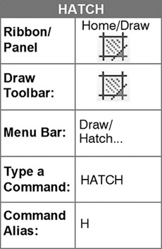
This crosshatching is done in AutoCAD by drawing hatch patterns. Exercise 8-3 will describe the HATCH command, used to draw hatch patterns.
When you have completed Exercise 8-3, your drawing will look similar to Figure 8-35.
Step 1. Begin drawing CH8-EXERCISE3 on the hard drive or network drive by opening existing drawing CH8-EXERCISE1 and saving it to the hard drive or network drive with the name CH8-EXERCISE3. You can use all the settings and text created for Exercise 8-1.
Step 2. Reset drawing limits, grid, and snap as needed.
Step 3. Create the following layers by renaming the existing layers and adding the a-sect-fixt layer.

Step 4. After looking closely at Figure 8-36, you may want to keep some of the conference room elevation drawing parts. Use Erase to eliminate the remainder of the drawing.

Figure 8-36 Exercise 8-3: Tenant space, section of conference room cabinets before hatching (scale: 3/4″ = 1′-0″)
Step 5. Change the underlined text to read CONFERENCE ROOM CABINET SECTION, change the top number in the balloon, and change the drawing scale to read as shown in Figure 8-36.
Step 6. Set the drawing annotation scale to ¾″ = 1′-0″.
Step 7. Use the correct layers and the dimensions shown in Figure 8-36 to draw the sectional view of the south wall of the tenant space conference room cabinets before using the HATCH command. Draw the section full size (measure features with an architectural scale of ¾″ = 1′ to find the correct size). Include the text and the dimensions. Your drawing will look similar to Figure 8-36 when it is completed prior to adding hatch patterns.
Step 8. When the cabinet section is complete with text and dimensions, freeze the a-sect-dims layer so it will not interfere with drawing the hatch patterns.
Prepare to Use the Hatch Command with the Add: Select Objects Boundary Option
When using the HATCH command there are two options for selecting the boundary of the area you will hatch; those two options are Add: Pick points and Add: Select objects. The Add: Select objects option requires additional preparation.
The most important aspect of using the HATCH command when you use Select Objects to create the boundary is to define clearly the boundary of the area to be hatched. If the boundary of the hatching area is not clearly defined, some of the hatch pattern may go outside the boundary area, or the boundary area may not be completely filled.
Before you use the HATCH command in this manner, all areas to which hatching will be added must be prepared so that none of their boundary lines extend beyond the area to be hatched. When the views on which you will draw hatching have already been drawn, it is often necessary to use the BREAK command to break the boundary lines into line segments that clearly define the hatch boundaries.
Step 9. Use the BREAK command to help clearly define the right edge of the horizontal plywood top of the upper cabinets (Figure 8-37), as described next:
Prompt |
Response |
Type a command: |
Break (or type BR <Enter>) |
Select object: |
P1→ (to select the vertical line) |
Specify second break point or [First point]: |
Type F <Enter> |
Specify first break point: |
P2→ (use Osnap-Intersection) |
Specify second break point: |
Type @ <Enter> (places the second point exactly at the same place as the first point, and no gap is broken out of the line) |
Type a command: |
<Enter> (repeat BREAK) |
Select object: |
P3→ (to select the vertical line) |
Specify second break point or [First point]: |
Type F <Enter> |
Specify first break point: |
P4→ (use Osnap-Intersection) |
Specify second break point: |
Type @ <Enter> |

Figure 8-37 Use the BREAK command to define clearly the right edge of the horizontal top area of the upper cabinets
You have just used the BREAK command with the @ option to break the vertical line so that it is a separate line segment that clearly defines the right edge of the plywood top area.
Tip
You can also use the Break at Point command from the Modify panel on the ribbon and eliminate typing F for first point.
Step 10. Use the BREAK command to define the bottom left edge of the plywood top boundary. Break the vertical line at the intersection of the bottom of the left edge (Figure 8-38).

Step 11. When the boundary of the plywood top is clearly defined, the top, bottom, right, and left lines of the top are separate line segments that do not extend beyond the boundary of the plywood top. To check the boundary, pick and highlight each line segment. Use the BREAK command on the top horizontal line of the plywood top, if needed (Figure 8-38).
Step 12. Use the BREAK command to prepare the three plywood shelves and the plywood bottom of the upper cabinet boundaries for hatching (Figure 8-38).
Step 13. The HATCH command will also not work properly if the two lines of an intersection do not meet, that is, if there is any small gap. If you need to check the intersections of the left side of the plywood shelves to make sure they intersect properly, do this before continuing with the HATCH command.
Tip
You may prefer to draw lines on a new layer over the existing ones to form the enclosed boundary area instead of breaking, as described in this procedure. These additional lines may be erased easily with a window after you turn off all layers except the one to be erased. This is sometimes faster and allows the line that was to be broken to remain intact.
Tip
If there is a small gap at the intersection of two lines, change the gap tolerance (HPGAPTOL) system variable. Type HPGAPTOL <Enter> at the command prompt. Any gaps equal to or smaller than the value you specify in the hatch pattern gap tolerance are ignored, and the boundary is treated as closed. You can also use the CHAMFER command (0 distance) or the FILLET command (0 radius) to connect two lines to form a 90° angle.
Use the Hatch Command with the Add: Select Objects Boundary Option
Step 14. Set layer a-sect-patt current.
Step 15. Use the HATCH command with the Add: Select objects boundary option to draw a uniform horizontal-line hatch pattern on the plywood top of the upper cabinets (Figure 8-39), as described next:
Prompt |
Response |
Type a command: |
Hatch (or type H <Enter>, |
Pick internal point or [Select objects seTtings]: |
T <Enter>) |
Click User-defined in the Type: area of Type and pattern: Angle: 0 Spacing: 1/4″ Click Add: Select objects |
|
Select objects or [picK internal point setTings]: |
(Figure 8-39) Click P1→ |
Specify opposite corner: |
Click P2→ |
Select objects or [picK internal point seTtings]: (A preview of your hatching appears): |
<Enter> (if the correct hatch pattern was previewed; if not, click <Esc> and fix the problem) |

Figure 8-39 Use the Hatch command with the Select Objects <Boundary> option to draw a uniform horizontal-line hatch pattern on the plywood top of the upper cabinets
Note
Although the Pick points method of creating hatch boundaries is often much easier, you must know how to use Select objects as well. There are instances when Pick points just does not work.
The plywood top of the upper cabinet is now hatched.
Step 16. Use the same hatching procedure to draw a hatch pattern on the three plywood shelves and the plywood bottom of the upper cabinet, as shown in Figure 8-40.

Figure 8-40 Draw a hatch pattern on the three plywood shelves and the plywood bottom of the upper cabinet
Tip
Turn off or freeze the text and dimension layers if they interfere with hatching.
Use the Hatch Command with the Add: Pick Points Boundary Option
When you use the Add: Pick points boundary option to create a boundary for the hatch pattern, AutoCAD allows you to pick any point inside the area, and the boundary is automatically created. You do not have to prepare the boundary of the area as you did with the Select objects boundary option, but you have to make sure there are no gaps in the boundary.
Step 17. Use the HATCH command with the Pick points boundary option to draw a uniform vertical-line hatch pattern on the upper cabinet door (Figure 8-41), as described next:
Prompt |
Response |
Type a command: |
Hatch (or type H <Enter> |
Pick internal point or [Select objects seTtings]: |
Type T |
The Hatch and Gradient dialog box appears: |
Click User-defined in the Type: area of Type and pattern: Angle: 90 Spacing: 1/4″ Click Add: Pick points |
Click P1 → (inside the door symbol) |
|
Pick internal point or [Select objects seTtings]: (A preview of your hatching appears): |
<Enter> (if the correct hatch pattern was previewed; if not, click <Esc> and fix the problem) |

Figure 8-41 Use the HATCH command with the Pick points boundary option to draw a uniform vertical-line hatch pattern on the upper cabinet door
Tip
You may have to draw a line across the top of the 5/8″ gypsum board to create the hatch pattern on the gypsum board.
Step 18. Use the HATCH command with the Pick points boundary option to draw the AR-SAND hatch pattern on the 5/8″ gypsum board (Figures 8-42, 8-43, and 8-44), as described next:
Prompt |
Response |
Type a command: |
Hatch |
Pick internal point or [select objects seTtings]: |
Type T<Enter> |
The Hatch and Gradient dialog box appears: |
Click Predefined (in the Type: area) Click ... (to the right of the Pattern: list box) |
The Hatch Pattern Palette appears: |
Click the Other Predefined tab Click AR-SAND (Figure 8-42) Click OK |


Note
When Associative is checked in the Hatch and Gradient dialog box, pick any point on the hatch pattern to erase it.
Response |
|
The Hatch and Gradient dialog box appears (Figure 8-43): |
Click 0 (in the Angle box) Type 3/8″ (in the Scale: box) Click Add: Pick points |
Pick internal point or [Select objects seTtings]: |
Click any point inside the lines defining the 5/8″ gypsum board boundary (Figure 8-44) |
Pick internal point or [Select objects seTtings]: |
<Enter> |
The 5/8″ gypsum board is now hatched. (If you get an error message, try 1/2″ for scale in the Scale: box or draw a line across the top of the gypsum board.)
Hatch; Hatch and Gradient Dialog Box; Hatch Tab
Type and Pattern
When the HATCH command is activated (type H <Enter>, then T <Enter>) the Hatch and Gradient dialog box with the Hatch tab selected appears (Figure 8-45). As listed in the Type and pattern: list box, the pattern types can be as follows:

Note
When you type H <Enter>, the Hatch Creation panel appears on the ribbon with most of the same features as the Hatch and Gradient dialog box. You may use either of these to define a hatch pattern.
Predefined: Makes the Pattern... button available.
User-defined: Defines a pattern of lines using the current linetype.
Custom: Specifies a pattern from the ACAD.pat file or any other PAT file.
To view the predefined hatch pattern options, click the ellipsis (...) to the right of the Pattern: list box. The Hatch Pattern Palette appears (Figure 8-46). Other parts of the Hatch and Gradient dialog box are as follows:
Pattern: Specifies a predefined pattern name.
Color: Allows you to use the current color or to choose another color for the hatch.
Background color: The area to the right of the Color box allows you to specify a background color for a hatch. The default color is none.
Custom pattern: This list box shows a custom pattern name. This option is available when Custom is selected in the Type: area.

Angle and Scale
Angle: Allows you to specify an angle for the hatch pattern relative to the X-axis of the current UCS.
Scale: This allows you to enlarge or shrink the hatch pattern to fit the drawing. It is not available if you have selected User-defined in the Type: list box.
Double: When you check this box, the area is hatched with a second set of lines at 90° to the first hatch pattern (available when User-defined pattern type is selected).
Relative to paper space: Scales the pattern relative to paper space so you can scale the hatch pattern to fit the scale of your paper space layout.
Spacing: Allows you to specify the space between lines on a user-defined hatch pattern.
ISO pen width: If you select one of the 14 ISO (International Organization for Standardization) patterns at the bottom of the list of hatch patterns and on the ISO tab of the Hatch Pattern Palette, this option scales the pattern based on the selected pen width. Each of these pattern names begins with ISO.
Hatch Origin
Controls where the hatch pattern originates. Some hatch patterns, such as brick, stone, and those used as shingles, need to start from a particular point on the drawing. By default, all hatch origins are the same as the current UCS origin.
Use current origin: Uses 0,0 as the origin by default. In most cases this will be what you want.
Specified origin: Specifies a new hatch origin. When you click this option, the following options become available.
Click to set new origin: When you click this box, you are then prompted to pick a point on the drawing as the origin for the hatch pattern.
Default to boundary extents: This option allows you to select a new origin based on the rectangular extents of the hatch. Choices include each of the four corners of the extents and its center.
Store as default origin: This option sets your specified origin as the default.
Preview button: Allows you to preview the hatch pattern before you apply it to a drawing.
Boundaries
Add: Pick points: Allows you to pick points inside a boundary to specify the area to be hatched.
Add: Select objects: Allows you to select the outside edges of the boundary to specify the area to be hatched.
Remove boundaries: Allows you to remove from the boundary set objects defined as islands by the Pick Points option. You cannot remove the outer boundary.
Recreate boundary: Allows you to create a polyline or a region around the hatch pattern.
View Selections: Displays the currently defined boundary set. This option is not available when no selection or boundary has been made.
Options
Annotative: You can make the hatch annotative by selecting the box beside Annotative under Options in the dialog box. To add the annotative hatch to your drawing, first, set the desired annotation scale for your drawing. Second, hatch the object (using type, pattern, angle, and scale) so you can see that the hatch is the correct size and appearance. If you change the plotting scale of your drawing, you can change the size of the hatch pattern by changing the annotation scale, located in the lower right corner of the status bar.
Associative: When a check appears in this button, the hatch pattern is a single object and stretches when the area that has been hatched is stretched.
Create separate hatches: When this button is clicked so that a check appears in it, you can create two or more separate hatch areas by using the HATCH command only once. You can erase those areas individually.
Draw order: The Draw order: list allows you to place hatch patterns on top of or beneath existing lines to make the drawing more legible.
Layer: Allows you to use the current layer for the hatch or to choose any other predefined layer.
Transparency: Allows you to use the current transparency setting for the hatch or to choose another setting.
Inherit Properties: Allows you to pick an existing hatch pattern to use on another area. The pattern picked must be associative (attached to and defined by its boundary).
More Options
When the More Options arrow in the lower right corner is clicked, the following options (Figure 8-47) appear.

Islands
The following Island display style options are shown in Figure 8-47:
Normal: When clicked (and a selection set is composed of areas inside other areas), alternating areas are hatched, as shown in the Island display style: area.
Outer: When clicked (and a selection set is composed of areas inside other areas), only the outer area is hatched, as shown in the Island display style: area.
Ignore: When clicked (and a selection set is composed of areas inside other areas), all areas are hatched, as shown in the Island display style: area.
Boundary Retention
Retain boundaries: Specifies whether the boundary objects will remain in your drawing after hatching is completed.
Object type: Allows you to select either a polyline or a region if you choose to retain the boundary.
Boundary Set
List box: This box allows you to select a boundary set from the current viewport or an existing boundary set.
New: When clicked, the dialog box temporarily closes and you are prompted to select objects to create the boundary set. AutoCAD includes only objects that can be hatched when it constructs the new boundary set. AutoCAD discards any existing boundary set and replaces it with the new boundary set. If you don’t select any objects that can be hatched, AutoCAD retains any current set.
Gap Tolerance
Allows a gap tolerance of between 0 and 5000 units to hatch areas that are not completely enclosed.
Inherit Options
Allows you to choose either the current hatch origin or the origin of the inherited hatch for the new hatch pattern.

Note
When you double-click on a hatch pattern, Hatch Editor appears on the ribbon. The Hatch Editor has most of the features of the Hatch Edit dialog box.
Edit Hatch
Select Edit Hatch... or type HE <Enter> and click on a hatch pattern to access the Hatch Edit dialog box (Figure 8-49). You can edit the pattern, angle, scale, origin, and draw order of the hatch pattern.


If you have an associative hatch pattern on a drawing that has one or two lines extending outside the hatch area, explode the hatch pattern. You may then trim the lines, because they are individual lines.
Step 19. Using the patterns described in Figure 8-50, draw hatch patterns by using the Pick points option on the lower cabinets and the end views of wood in the upper cabinets.

Step 20. Thaw frozen layers.
Step 21. When you have completed Exercise 8-3 (Figure 8-51), save your work in at least two places.

Figure 8-51 Exercise 8-3: Completed section drawing (scale: 3/4″ = 1′-0″)
Step 22. Print Exercise 8-3 at a scale of 3/4″ = 1′-0″.
Step 23. Add the section symbol as shown in Figure 8-52 to your TENANT SPACE FLOOR PLAN drawing. Use a 1′-radius circle and 1/16″-high text (annotative). You may need to move two dimensions as shown and add a layer for the cutting plane line below the symbol. Use PHANTOM 2 linetype and .004″ lineweight, color red.

EXERCISE 8-4 Detail of Door Jamb with Hatching
In Exercise 8-4, a detail of a door jamb is drawn. When you have completed Exercise 8-4, your drawing will look similar to Figure 8-53.

Figure 8-53 Exercise 8-4: Detail of a door jamb with crosshatching (scale: 3″ = 1′-0″)
Step 1. Use your workspace to make the following settings:
1. Use Save As... to save the drawing on the hard drive with the name CH8-EXERCISE4.
2. Set drawing units, limits, grid, and snap.
3. Create the following layers:

4. Set layer a-detl-lwt1 current.
Step 2. Using the dimensions shown in Figure 8-53, draw all the door jamb components. Drawing some of the components separately and copying or moving them into place will be helpful. Measure any dimensions not shown with a scale of 3″ = 1′-0″.
Step 3. Set layer a-detl-patt current, and draw the hatch patterns as described in Figure 8-54. Use a spline and array it to draw the curved wood grain pattern.

Figure 8-54 Exercise 8-4: Hatch patterns
Step 4. Set layer a-detl-dims current, set the dimensioning variables, and draw the dimensions as shown in Figure 8-53.
Step 5. Set layer a-detl-text current, and add the name of the detail as shown in Figure 8-53. Add your name, class, and current date in the upper right.
Step 6. Save the drawing in two places.
Step 7. Print the drawing at a scale of 3″ = 1′-0″.
EXERCISE 8-5 Use Point Filters and OTRACK to Make an Orthographic Drawing of a Conference Table
In Exercise 8-5, the AutoCAD features called point filters and OTRACK are used. These features are helpful when you are making 2D drawings showing the top, front, and side views of an object. All the features in these views must line up with the same features in the adjacent view. When you have completed Exercise 8-5, your drawing will look similar to Figure 8-55.

Figure 8-55 Exercise 8-5: Use point filters and OTRACK to draw three views of a dining table (scale: 1/2″ = 1′-0″)
point filters: A method of entering a point by which the X, Y, and Z coordinates are given in separate stages. Any one of the three coordinates can be first, second, or third.
OTRACK: A setting that allows you to specify points by hovering your pointing device over osnap points.
Step 1. Use your workspace to make the following settings:
1. Set drawing units: Architectural
2. Set drawing limits: 16′,14′
3. Set GRIDDISPLAY: 0
4. Set grid: 2″
5. Set snap: 1″
6. Create the following layers:

7. Set Layer2 current.
8. Set LTSCALE: 16.
9. Save the drawing as CH8-EXERCISE5.
Step 2. Draw the base and column of the table (hidden line), as shown in the top view (Figure 8-56), as described next:
Prompt |
Response |
Type a command: |
Circle-Center, Diameter (not Radius) |
Specify center point for circle or [3P 2P Ttr (tan tan radius)]: |
Type 4′,9′<Enter> |
Type 2′2 <Enter> |
|
Type a command: |
Circle-Center, Diameter (not Radius) |
Specify center point for circle or [3P 2P Ttr (tan tan radius)]: |
Type 4′,9′ (the same center as the first circle) |
Specify diameter of circle <default>: |
Type 2 <Enter> |

Step 3. Set Layer1 current.
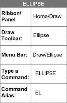
Step 4. Draw the elliptical top of the table (continuous linetype), as shown in the top view (Figure 8-56), as described next:
Prompt |
Response |
Type a command: |
Ellipse-Center |
Specify center of ellipse: |
Osnap-Center |
of |
P1→ |
Specify endpoint of axis: |
With ORTHO on, move your mouse up and type 2′ <Enter> |
Specify distance to other axis or [Rotation]: |
Type 39 <Enter> |
Point Filters
Step 5. Use point filters to draw the front view of the top of this elliptical table (Figure 8-57), as described next:
Response |
|
Type a command: |
Line |
Specify first point: |
Type .X <Enter> |
of |
Osnap-Quadrant |
of |
P1→ (Figure 8-57) |
(need YZ): |
P2→ (with SNAP on, pick a point in the approximate location shown in Figure 8-57) |
Specify next point or [Undo]: |
Type .X <Enter> |
of |
Osnap-Quadrant |
of |
P3→ |
(need YZ): |
P4→ (with ORTHO on, pick any point to identify the Y component of the point; ORTHO makes the Y component of the new point the same as the Y component of the previous point) |
Specify next point or [Close Undo]: |
With ORTHO on, move your mouse straight down, and type 1 <Enter> |
Specify next point or [Close Undo]: |
Type .X <Enter> |
of |
Osnap-Endpoint |
of |
(Figure 8-57) P2→ |
(need YZ): |
With ORTHO on, move your mouse to the right, and pick any point |
Specify next point or [Close Undo]: |
Type C <Enter> |

OTRACK
Step 6. Set running Osnap modes of Endpoint, Quadrant, and Intersection and turn OSNAP and OTRACK on.
Step 7. Use OTRACK and Offset to draw the front view of the column (Figure 8-58), as described next:
Prompt |
Response |
Type a command: |
Line |
Specify first point: |
Move your mouse to the right quadrant shown as P1→ (Figure 8-58) but do not click |
Hold it until the quadrant symbol appears, then move your mouse straight down until the dotted line shows the intersection symbol on the bottom line of the tabletop as shown, then click the intersection point (Figure 8-58) |
|
Specify next point or [Undo]: |
With ORTHO on, move your mouse straight down and type 27 <Enter> |
Specify next point or [Undo]: |
<Enter> |
Type a command: |
Offset (or type O <Enter>) |
Specify offset distance or [Through Erase Layer] <Through>: |
Type 2 <Enter> |
Select object to offset or [Exit Undo] <Exit>: |
Click P1→ (Figure 8-59) |
Specify point on side to offset or [Exit Multiple Undo] <Exit>: |
Click P2→ (any point to the left of the 27″ line) |
Select object to offset or [Exit Undo] <Exit>: |
<Enter> |


Step 8. Use OTRACK to draw the front view of the base (Figure 8-59), as described next:
Prompt |
Response |
Type a command: |
Line |
Specify first point: |
Move your mouse to the quadrant shown as P3→ (Figure 8-59) but do not click Hold it until the quadrant symbol appears, then move your mouse to P4→ (do not click) (the dotted line shows the endpoint symbol), then move your mouse back to the vertical dotted tracking line and click |
Specify next point or [Undo]: |
With ORTHO on, move your mouse straight down and type 1 <Enter> |
Specify next point or [Undo]: |
With ORTHO on, move your mouse to the left and type 26 <Enter> |
Specify next point or [Close Undo]: |
With ORTHO on, move your mouse straight up, and type 1 <Enter> |
Specify next point or [Close Undo]: |
Type C <Enter> |
Step 9. Use OTRACK to draw the right-side view of the table with the LINE and COPY commands (Figure 8-60). Be sure to get depth dimensions from the top view.

Figure 8-60 Draw the right-side view using COPY, LINE, and OTRACK. Complete front and right-side views with a 5″ no trim radius and the TRIM command
Step 10. Use a 5″-radius fillet (no trim) and trim to complete front and right-side views.
Step 11. Set Layer3 current. Label the drawing as shown in Figure 8-55. Add your name, class, and current date in the upper right.
Step 12. Save your drawing in two places.
Step 13. Print the drawing at a scale of 1/2″ = 1′-0″.
Chapter Summary
This chapter provided you the information necessary to set up and draw interior elevations, sections, and details. The UCS and UCS Icon commands were used extensively in drawing the elevations. In addition, the Multileader command was explored in detail, and point filters and OTRACK were used to draw 2D views. Now you have the skills and information necessary to produce elevations, sections, and drawing details that can be used in interior design sales pieces, information sheets, contract documents, and other similar types of documents.
Chapter Test Questions
Multiple Choice
Circle the correct answer.
1. The W on the 2D UCS icon indicates which of the following?
a. face
b. view
c. world
d. object
2. Which of the following angles produces the user-defined pattern shown in Figure 8-61?
a. 45
b. 90
c. 0
d. 135

3. Which of the following angles produces the user-defined pattern shown in Figure 8-62?
a. 45
b. 90
c. 0
d. 135

4. Which of the following commands can be used to correct a hatch pattern that extends outside a hatch boundary, after it has been exploded?
a. ARRAY
b. COPY
c. MOVE
d. TRIM
5. When the Noorigin option of the UCS Icon is selected, where is the UCS Icon displayed?
a. The lower left corner of the screen.
b. It is turned off.
c. It moves to the new UCS origin.
d. It rotates.
6. Which of the following tabs is used to set the landing distance of a multileader?
a. Leader Format
b. Leader Structure
c. Content
d. Attachment
7. The Multileader Collect command can be used to:
a. Align leaders
b. Add leaders
c. Change a circle to a hexagon
d. Attach multiple balloons to one leader
8. Which setting allows an image to be mirrored without mirroring the text?
a. MIRRTEXT = 1
b. MIRRTEXT = 0
c. MIRRTEXT = 3
d. DTEXT-STYLE = 0
9. The STRETCH command is best used for:
a. Stretching an object in one direction
b. Moving an object along attached lines
c. Shrinking an object on one direction
d. All of the above
10. Which of the following is an option in the Boundaries area of the Hatch and Gradient dialog box?
a. Find boundaries
b. Subtract boundaries
c. Remove boundaries
d. Define boundaries
Matching
Write the number of the correct answer on the line.

True or False
Circle the correct answer.
1. True or False: The Coordinates panel is hidden in the View tab of the ribbon by default.
2. True or False: A multileader can be drawn with content first only.
3. True or False: You must clearly define the boundary of the area to be hatched when you use the Add: Select Objects option of the Hatch command.
4. True or False: Origin is the name of the UCS Icon command option that forces the UCS icon to be displayed at the 0,0 point of the current UCS.
5. True or False: Picking any point on an associative 35-line hatch pattern with the ERASE command and then pressing <Enter> will erase it.
2. Five commands of the Modify panel under the Draw Ribbon tab.
3. Five options of the Lengthen command.
4. Five options of the Osnap menu that begin with M or N.
5. Five options available once the UCS command is launched.
6. Five ways of accessing the Multileader Style dialog box.
7. Five ways of accessing the Multileader command.
8. Five options of the Multileader Style Manager/Modify dialog box.
9. Five options under the Multileader command.
10. Five options of the Hatch and Gradient dialog box.
Questions
1. What is a user coordinate system and how is it used?
2. What are predefined hatch patterns and how are they used?
3. How are point filters and OTRACK similar?
4. When would you use multileaders?
5. How were the STRETCH and MIRROR commands used in this chapter, and how could you use them in the future?
Chapter Projects
Project 8-1: Detail Drawing of a Bar Rail [BASIC]
1. Draw the bar rail detail shown in Figure 8-63. Measure the drawing with an architectural 1/2 scale and draw it full size (1:1) using AutoCAD.

Figure 8-63 Project 8-1: Bar rail detail
2. Set your own drawing limits, grid, and snap. Create your own layers with varying lineweights as needed.
3. Label the drawing as shown in Figure 8-63 in the City Blueprint font. Add your name, class, and the current date in the upper right.
4. Save the drawing in two places and print the drawing at a scale of 1:2.
Project 8-2: Wheelchair-Accessible Commercial Restrooms Elevation [INTERMEDIATE]
Figure 8-64 shows the floor plan of the commercial restrooms with the elevations indicated. The line of text at the bottom of Figure 8-65 shows where the House Designer drawing is located in the AutoCAD DesignCenter. The front view of the toilets, urinals, sinks, grab bars, faucets, and toilet paper holders are blocks contained within this drawing and in Autodesk Seek design content online. Just double-click on any of these blocks to activate the INSERT command and insert these blocks into your elevation drawing as needed. You may need to modify the sink, and you will have to draw the mirror and paper towel holder.

Figure 8-64 Project 8-2: Floor plan of the wheelchair-accessible commercial restrooms (scale: 3/16″ = 1′-0″)

Figure 8-65 Project 8-2: House Designer blocks in the DesignCenter
Draw elevation 1 of the commercial wheelchair-accessible restrooms as shown in Figure 8-66. Use the dimensions shown or use an architectural scale of 3/16″ = 1′0″ to measure elevation 1, and draw it full scale without dimensions. Use lineweights to make the drawing more attractive and a solid hatch pattern with a gray color to make the walls solid. Use the same gray color for the layer on which you draw the ceramic tile. When you have completed Project 8-2, your drawing will look similar to Figure 8-66. You may locate drawings of the sinks and urinal that are a little different from those shown on this drawing. If so, use them. Just be sure they are located correctly. Add dimensions as required. Save the drawing in two places and print the drawing to scale.

Figure 8-66 Project 8-2: Wheelchair-accessible commercial restrooms elevation (scale: 3/16″ = 1′-0″)
Project 8-3: Drawing a Mirror and Sections of a Mirror from a Sketch [ADVANCED]
1. Use the dimensions shown to draw the mirror in Figure 8-67 using AutoCAD.

Figure 8-67 Project 8-3: Mirror
2. Set your own drawing limits, grid, and snap. Create your own layers as needed.
3. Do not place dimensions on this drawing, but do show the cutting plane lines and label them as shown.
4. Do not draw Detail A. This information is shown so you can draw that part.
5. Draw and label sections A-A, B-B, and C-C in the approximate locations shown on the sketch. Use the ANSI31 hatch pattern for the sectional views, or draw splines and array them to show wood. Do not show dimensions.
6. Save the drawing in two places and print the drawing to scale.
Project 8-4, Part 1: Log Cabin Kitchen Elevation 1 [BASIC]
Figure 8-68 shows the floor plan of the log cabin kitchen with two elevations indicated. The line of text at the bottom of Figure 8-69 shows where the Kitchen drawing is located in the AutoCAD DesignCenter. The front view of the dishwasher, faucet, range-oven, and refrigerator are blocks contained within this drawing. Just double-click on any of these blocks to activate the INSERT command, and insert these blocks into your elevation drawing as needed.

Figure 8-68 Project 8-4: Plan view of the log cabin kitchen

Figure 8-69 Project 8-4: DesignCenter with the Kitchen drawing blocks displayed
Draw elevation 1 of the log cabin kitchen as shown in Figure 8-70. Use the dimensions shown or use an architectural scale of 1/2″ = 1′0″ to measure elevation 1, and draw it full scale with dimensions. Use lineweights to make the drawing more attractive and a solid hatch pattern with a gray color to make the walls solid.

Figure 8-70 Project 8-4, Part 1: Log cabin kitchen elevation 1 (scale: 1/2″ = 1′–0″)
When you have completed Project 8-4, Part 1, your drawing will look similar to Figure 8-70 with dimensions. Save the drawing in two places and print the drawing to scale.
Project 8-4, Part 2: Log Cabin Kitchen Elevation 2 [BASIC]
Figure 8-68 shows the floor plan of the log cabin kitchen with arrows indicating the line of sight for two elevations of this room. The line of text at the bottom of Figure 8-69 shows where the Kitchen drawing is located in the AutoCAD DesignCenter. The front view of the dishwasher, faucet, range-oven, and refrigerator are blocks contained within this drawing. Just double-click on any of these blocks to activate the INSERT command, and insert these blocks into your elevation drawing as needed.
Draw elevation 2 of the log cabin kitchen as shown in Figure 8-71. Use the dimensions shown or use an architectural scale of 1/2″ = 1′0″ to measure elevation 2, and draw it full scale with dimensions. Use lineweights to make the drawing more attractive and a solid hatch pattern with a gray color to make the walls solid.

Figure 8-71 Project 8-4, Part 2: Log cabin kitchen elevation 2 (scale: 1/2″ = 1′–0″)
When you have completed Project 8-4, Part 2, your drawing will look similar to Figure 8-71 with dimensions. Save the drawing in two places and print the drawing to scale.
Project 8-5: Family Room, House 1 Elevation [ADVANCED]
Project 8-5 is an elevation of the family room, house 1, Figure 8-72, Sheet 1. When you have completed Project 8-5, your drawing will look like that figure with dimensions added.

Figure 8-72 Sheet 1 of 2 Project 8-5: House 1 family room elevation (scale: 3/8″ = 1′-0″)
Measure the features in the elevation using the scale indicated and draw them full scale.
Use the dimensions in Figure 8-72, Sheet 2 for some of the details. Add dimensions to the elevation as required. Save the drawing in two places and plot or print the drawing to scale.

Figure 8-72 Sheet 2 of 2 Dimensions for Project 8-5