Chapter 12
Keeping In Control with Constraints
Constraints are specific restrictions applied to objects that allow for design exploration while maintaining object shape and/or size within predefined limits. In this chapter, you will create three types of constraints in the AutoCAD® 2014 program: geometric, dimensional, and user-created. Once the design has been sufficiently constrained, you will make a host of geometric and dimensional changes simply by changing a single parameter.
- Working with geometric constraints
- Applying dimensional constraints and creating user parameters
- Constraining objects simultaneously with geometry and dimensions
- Making parametric changes to constrained objects
Working with Geometric Constraints
Geometric constraints allow you to force specific 2D objects to be coincident, collinear, concentric, parallel, perpendicular, horizontal, vertical, tangent, smooth, and symmetric; to have equal lengths; or to be fixed in world space. In the following steps, you will assign sufficient geometric constraints to ensure that a rectangle will always remain square even when it is stretched:
The AutoCAD LT® program cannot create constraints. However, AutoCAD LT users can view and edit constraints that were created in AutoCAD 2014.
The sample files in this chapter use generic units so that they can be used by both Imperial and metric users.
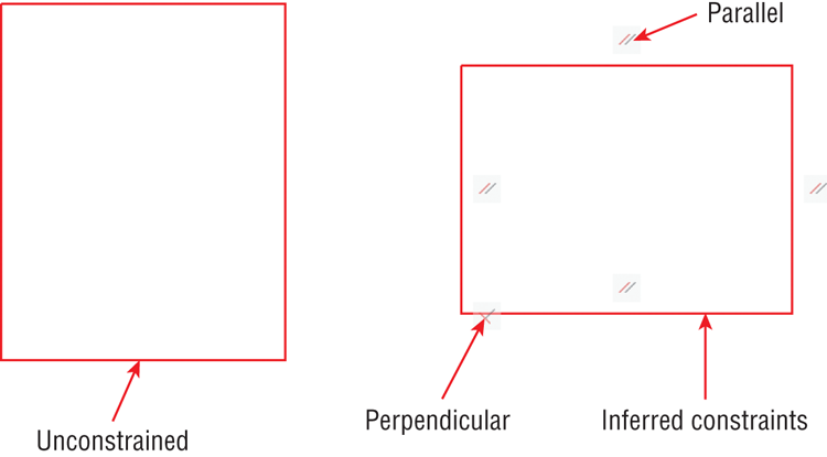
2. Select the Rectangle tool on the Draw panel. Click two points on the drawing canvas to create an arbitrarily sized rectangle.
3. Toggle Infer Constraints mode on in the status bar.
4. Press the spacebar to repeat the
RECTANG (for Rectangle) command, and then click two more points to draw another arbitrarily sized rectangle adjacent and to the right of the first one (see
Figure 12-1). AutoCAD automatically infers perpendicular and parallel constraints from the geometry of the second rectangle.
Parallel, collinear, concentric, and equal constraints always appear in pairs.
5. Toggle off Infer Constraints mode by pressing Ctrl+Shift+I.
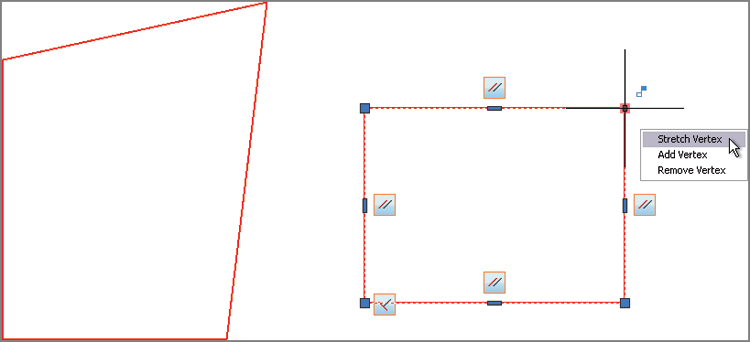
6. Select both rectangles with a crossing selection window. Hover the cursor over the upper-right grip of the left rectangle, select Stretch Vertex from the grip menu that appears, and stretch it up and to the right so that the rectangle deforms. Hover the cursor over the upper-right grip of the right rectangle, select Stretch Vertex from the grip menu, stretch it up and to the right, and click to set its new location. The rectangle remains a rectangle because of the constraints (see
Figure 12-2). Press Esc to deselect.
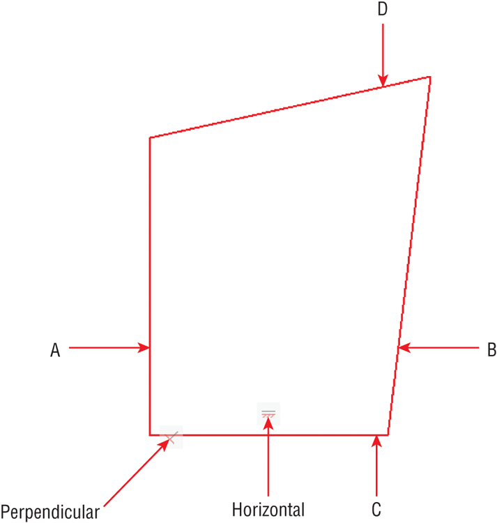
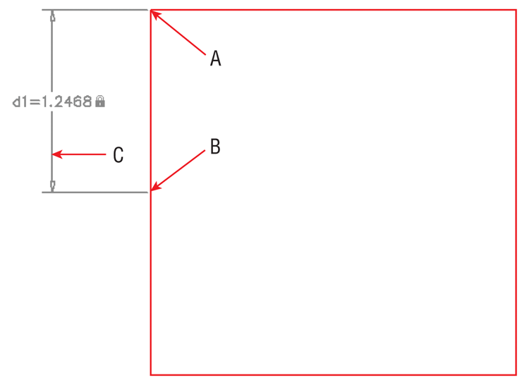
7. Select the Parametric tab on the ribbon, and select the Auto Constrain tool in the Geometric panel. Select the unconstrained rectangle on the left and press Enter. Two constraints are applied: perpendicular and horizontal (see
Figure 12-3).
Objects are never repositioned when inferring constraints or when using the Auto Constrain tool. Objects can be repositioned when applying constraints manually.
8. Select the Parallel constraint tool in the Geometric panel. Click lines A and B, as shown in
Figure 12-3. Line B is automatically repositioned to conform to the parallel constraint applied to line A.
The order in which you select objects can be significant when you apply constraints. The second object will be repositioned in some cases, depending on the constraint that is applied and the shape and position of the objects.
9. Press the spacebar to repeat the
GCPARALLEL (for Geometric Constraint Parallel) command. Click lines C and D, as shown in
Figure 12-3.
10. The left rectangle not only has parallel and perpendicular constraints like the right rectangle, but it also has a horizontal constraint that was applied by the Auto Constrain tool. Select the right rectangle, and press the Delete key.
11. Select the Equal constraint tool in the Geometric panel. Click lines A and C, as shown in
Figure 12-3. The rectangle becomes a square (see
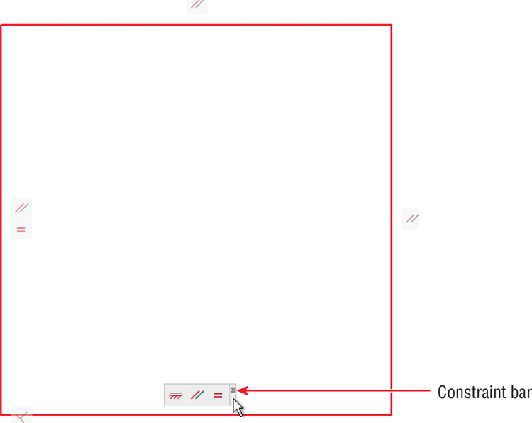
Figure 12-4).
12. Multiple constraints are grouped together in what is called a constraint bar. Position the cursor over the constraint bar, and you’ll see a tiny Close box. Click it to hide the constraint bar.
Hiding constraints does not remove them; it merely reduces visual clutter.
13. Click the Show All button in the Geometric panel. The hidden constraint bar reappears.
14. Right-click the horizontal constraint, and choose Delete from the context menu. The rectangle is no longer constrained horizontally (so you could rotate it if desired).
15. Click the Hide All button in the Geometric panel. The constraints are hidden but still active.
16. Save your work as Ch12-B.dwg.
Applying Dimensional Constraints and Creating User Parameters
Dimensional constraints allow you to control object sizes with specific numerical values and to set up dynamic dimensional relationships with mathematical equations and formulas. User constraints are not tied to specific geometry but hold values calculated from dimensional constraints. In the following steps, you will create dimensional and user constraints:
1. If the file is not already open from performing the previous step, go to the book’s web page, browse to Chapter 12, get the file Ch12-B.dwg, and open it.
2. Select the ribbon’s Home tab, open the Layer drop-down menu in the Layers panel, and select Layer 2 to make it the current layer.
3. Select the Parametric tab on the ribbon. Select the Linear constraint tool in the Dimensional panel, and click
constraint points A and B, as shown in
Figure 12-5. Constraint points highlight in red on screen when you move the cursor near them. Click point C to locate the dimension line. Press Enter to accept the default dimension text. This dimensional constraint is automatically given the variable name
d1.
Constraint points behave similarly to object snaps but are limited to endpoints, midpoints, center points, and insertion points.
4. Type C (for Circle), and press Enter. Draw an arbitrarily sized circle anywhere within the square.
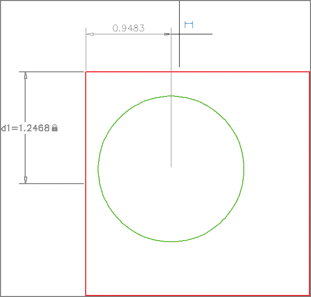
5. Click the Linear constraint tool in the Dimensional panel, and click the first constraint point in the upper-left corner of the rectangle. Click the circle to accept its center as the second constraint point. Move the cursor upward (see
Figure 12-6), and click to place the horizontal dimension line above the rectangle. Move on to step 6 without pressing Enter.
6. Type d2=d1, and press Enter. The circle moves over so that it is horizontally centered within the rectangle and the constraint reads fx: d2=d1. The fx means the dimensional constraint is calculated by a function.
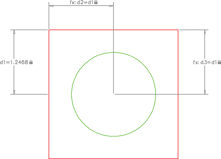
7. Press the spacebar to repeat the
DCLINEAR (for Dimensional Constraint Linear) command. Click the first constraint point in the upper-right corner of the rectangle. Click the circle to accept its center as the second constraint point. Move the cursor to the right, and click to place the vertical dimension line to the right of the rectangle. Type
d3=d1, and press Enter. The circle is now centered within the square (see
Figure 12-7).
You can convert an existing dimension into a dimensional constraint with the
DIMCONSTRAINT command.
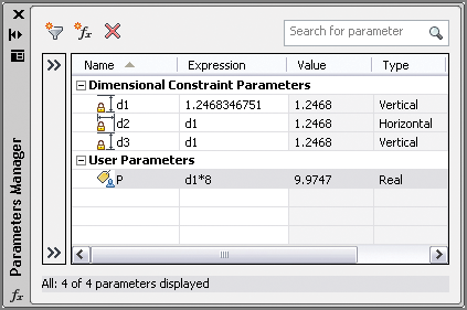
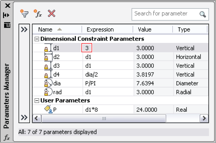
8. Click the Parameters Manager button in the Manage panel to open the Parameters Manager. All the dimensional constraints that you have created are listed here (d1, d2, and d3). Click the ƒx button to create a new user parameter.
9. Type
P (for Perimeter) as the user parameter name and press Enter. Double-click the Expression value, type
d1*8 (d1 times 8), and press Enter (see
Figure 12-8). The perimeter of the square is equal to eight times the length of half of one of its sides. Close the Parameters Manager.
10. Select the Hide All button in the Dimensional panel.
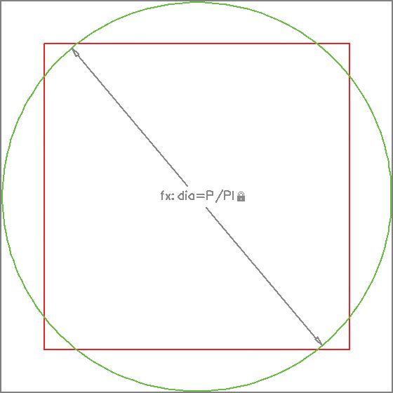
11. Select the Diameter constraint tool in the Dimensional panel, select the circle, click a point inside the circle to locate the dimension line, type
dia=P/PI, and press Enter. The variable PI is hard-coded as 3.14159265; there is no need to define it as a user variable. The circumference of the circle is now equal to the perimeter of the square, traditionally called
squaring the circle (see
Figure 12-9).
You can give constraints any name you like. I identified the diameter constraint with the letters
dia to represent the green circle’s diameter. If you wanted later to constrain the diameter of another circle, you might call it
dia2, for example.
12. Save your work as Ch12-C.dwg.
Constraining Objects Simultaneously with Geometry and Dimensions
You can use geometric and dimensional constraints together to force objects to conform to your design intent. In the following steps, you will draw two more circles and constrain their positions and sizes using a combination of geometric and dimensional constraints:
1. If the file is not already open, go to the book’s web page, browse to Chapter 12, get the file Ch12-C.dwg, and open it.
2. Select the ribbon’s Home tab, open the Layer drop-down menu in the Layers panel, and select Layer 3 to make it the current layer.
3. Type C (for Circle), and press Enter. Draw an arbitrarily sized circle anywhere within the square.
4. Select the ribbon’s Parametric tab, and then click the Concentric constraint tool in the Geometric panel. Select the green circle and then the blue circle. The blue circle immediately moves to conform to the geometric constraint so that it is concentric within the larger circle.
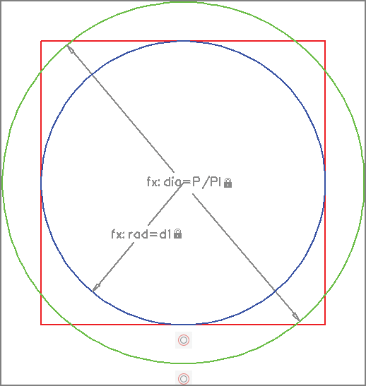
5. Select the Radius constraint tool in the Dimensional panel, select the blue circle, and click a point inside the circle to locate the dimension line. Type
rad=d1, and press Enter. The blue circle changes size so that it fits perfectly within the square (see
Figure 12-10).
6. Select the Hide All button in the Dimensional panel.
7. Select the ribbon’s Home tab, open the Layer drop-down menu in the Layers panel, and select Layer 4 to make it the current layer.
8. Type C (for Circle), and press Enter. Draw an arbitrarily sized circle anywhere above the square.
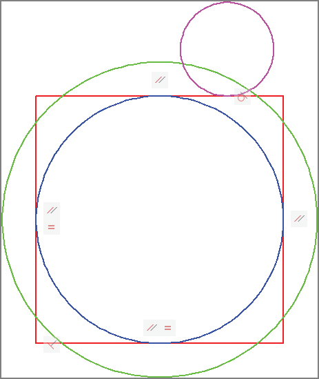
9. Select the ribbon’s Parametric tab, and click the Tangent constraint tool in the Geometric panel. Select the top line of the square as the first object and the magenta circle as the second object. The circle moves down to conform to the tangent constraint (see
Figure 12-11).
10. Press the spacebar to repeat the GCTANGENT (for Geometric Constraint Tangent) command. Select the blue circle first, and then select the magenta circle. The magenta circle moves on top of the blue circle to conform to the new tangent constraint.
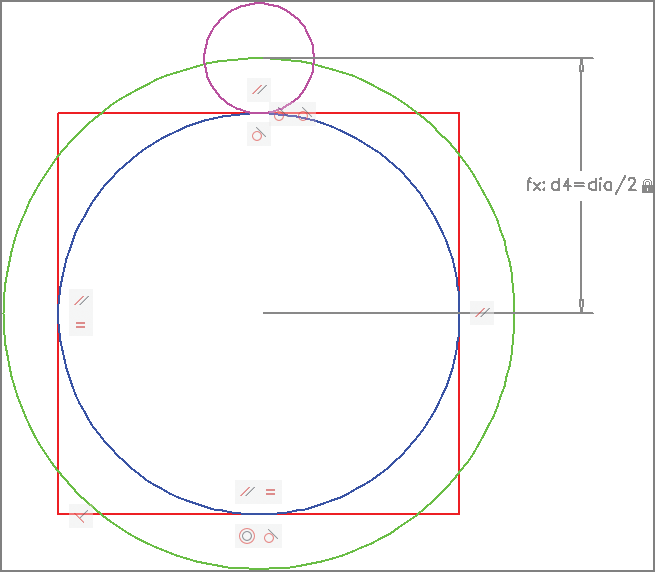
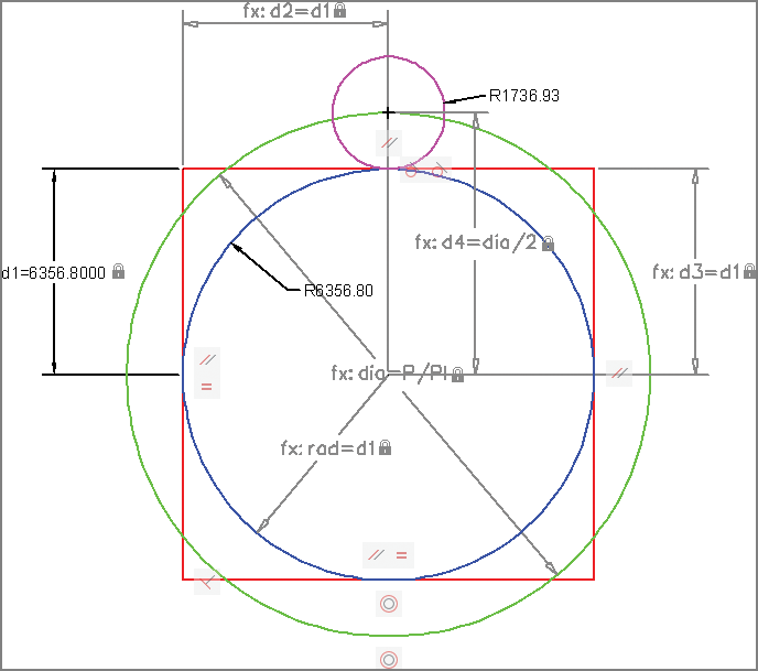
11. Click the Linear constraint tool in the Dimensional panel. Click the magenta circle, the blue circle, and then a point off to the right to place the dimension line. Type
d4=dia/2, and press Enter (see
Figure 12-12). The center of the magenta circle is anchored effectively at the top quadrant (or top cardinal point) of the green circle.
12. Click the Hide All button in the Dimensional panel, and click the Hide All button in the Geometric panel. All constraints are hidden but still active.
13. Save your work as Ch12-D.dwg.
Making Parametric Changes to Constrained Objects
Once you have intelligently applied geometric and/or dimensional constraints, it is easy to make parametric changes that affect the shape and/or size of multiple interconnected objects. In the following steps, you will change a single parameter (d1) and see how it affects the objects you have constrained. In addition, you will add dimensions to two circles and uncover an amazing coincidence.
1. If the file is not already open, go to the book’s web page, browse to Chapter 12, get the file Ch12-D.dwg, and open it.
2. Select the ribbon’s Parametric tab, and click the Parameters Manager button in the Manage panel.
3. Double-click the
d1 parameter’s expression. Type
3, and press Enter. All parameter values are recalculated because they are all based on the first parameter you created earlier in this chapter (see
Figure 12-13).
4. Click the Zoom Extents tool in the Navigation bar. The form of the diagram remains unchanged; only the scale has changed.
5. The Earth’s polar radius is 3949.9 miles (or 6356.8 km). Double-click the d1 parameter’s expression. Type 6356.8, and press Enter. Close the Parameters Manager.
6. Click the Zoom Extents tool in the Navigation bar.
7. Select the ribbon’s Home tab, open the Layer drop-down menu in the Layers panel, and select 0 to make it the current layer.
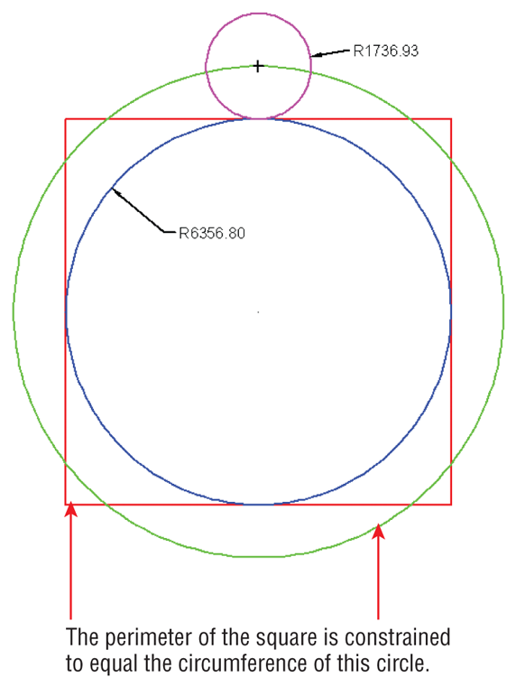
8. Select the ribbon’s Annotate tab, open the Dimension menu in the Dimensions panel, and click the Radius tool. Select the blue circle, and then click a point inside the circle to locate the dimension object.
9. Press the spacebar to repeat the
DIMRADIUS (Dimension Radius) command. Select the magenta circle, and click a point outside the circle to locate the dimension object.
Figure 12-14 shows the result.
10. The Moon’s polar radius is 1078.7 miles (or 1735.97 km). The diagram amazingly encodes the sizes of Earth and Moon with accuracy exceeding 99.9 percent. Your drawing should now resemble Ch12-E.dwg, which is available on the book’s web page.
John Michell was the first to discover this geometric relationship in his book
City of Revelation (Ballantine Books, 1973).
The Essentials and Beyond
In this chapter, you learned how to apply constraints to cause objects to conform to specific geometric, dimensional, and formulaic requirements. You saw how modifying constraint expressions makes objects automatically change their shapes and sizes to conform to the sum total of all applied constraints.
Additional Exercise
Explore annotational constraints on your own. For example, show all dimensional constraints, and then select the d1 constraint and open the Properties palette. Change the Constraint Form property to Annotational. Annotational constraints cannot be hidden but instead annotate the drawing, somewhat like dimension objects. However, the padlock symbol identifies them as dimensional constraints.