Chapter 5
Shaping Curves
For many years, the AutoCAD® program wasn’t very sophisticated when it came to shaping curves. Sure, you could create circles, arcs, and ellipses, but shaping complex curves wasn’t accurate compared to the capabilities of programs such as Autodesk® Maya® or Autodesk® 3ds Max®. In AutoCAD 2011, all this changed with the introduction of an all-new SPLINE command that offered much more flexibility in shaping true NURBS (nonuniform rational B-spline) curves using fit points or control vertices. AutoCAD 2014 expands on this by giving you the ability to shape curves in any way you can imagine and even use them to model surfaces, which you’ll learn more about in Chapter 17, “Modeling in 3D.”
- Drawing and editing curved polylines
- Drawing ellipses
- Drawing and editing splines
- Blending between objects with splines
Drawing and Editing Curved Polylines
The simplest curved objects are circles and arcs (which are just parts of circles), because they curve with a constant radius from a center point. In the following steps, you will chain a series of arcs and/or lines together in a single polyline object, which not only streamlines editing and selection but also ensures smooth curvature between adjacent arcs.
1. Go to the book’s web page at
www.sybex.com/go/autocad2014essentials, and browse to Chapter 5 to get the files
Ch5-A.dwg (or
Ch5-A-metric.dwg) and
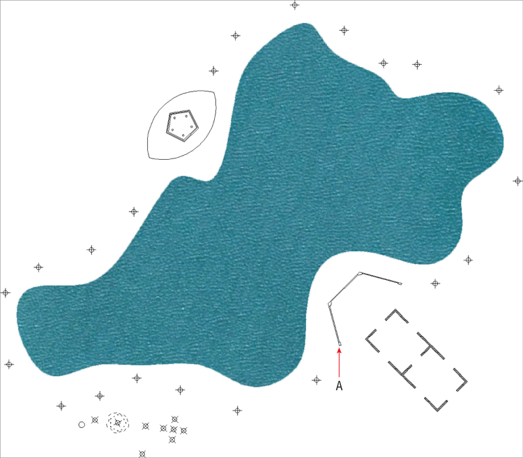
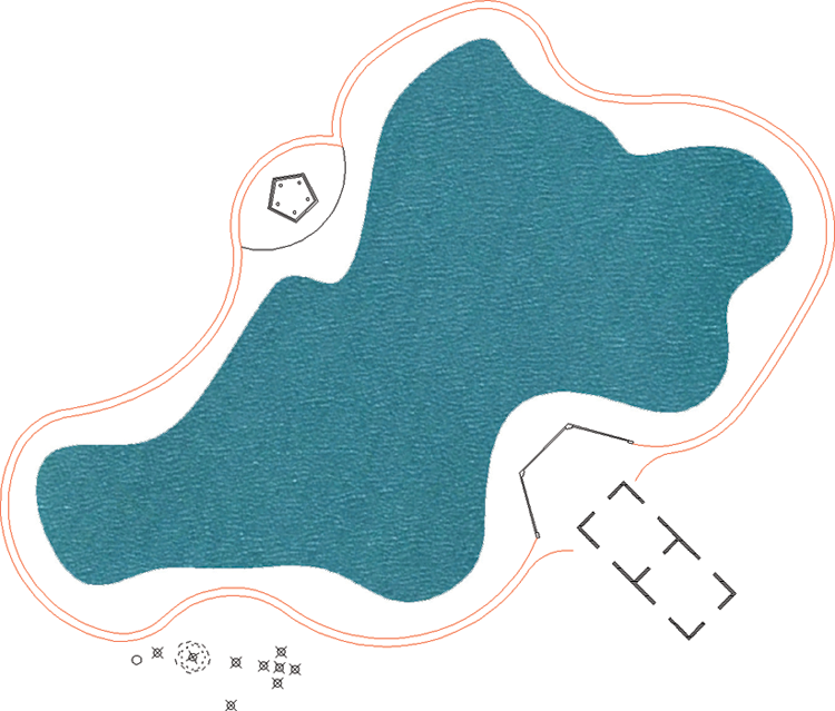
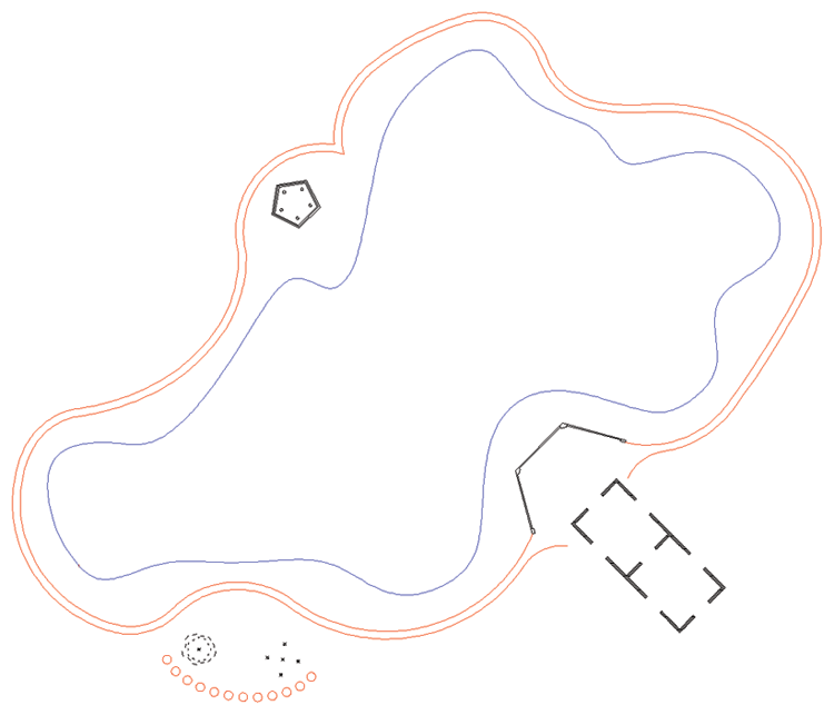
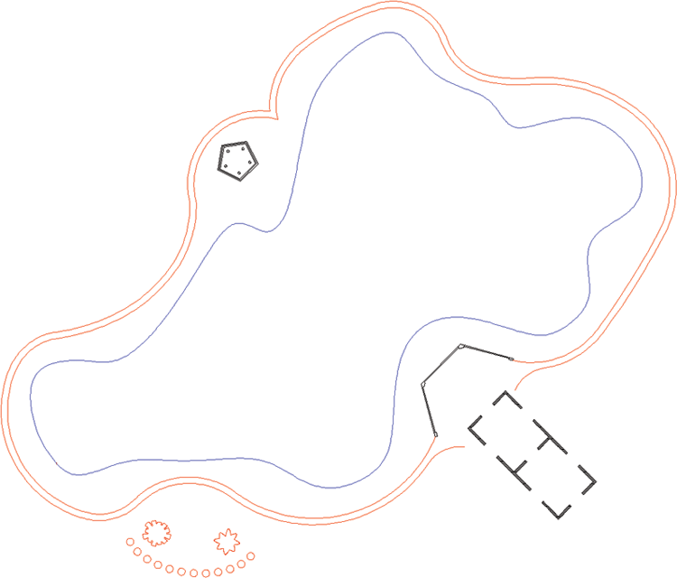
Pond.jpg. Place them in the same folder on your hard drive, and open the drawing file in AutoCAD (see
Figure 5-1).
2. You will begin by drawing curved pathways surrounding the lake. Click the Polyline tool on the Draw panel of the ribbon. Click the first point at point A as shown in
Figure 5-1. Type
A (for Arc), and press Enter.
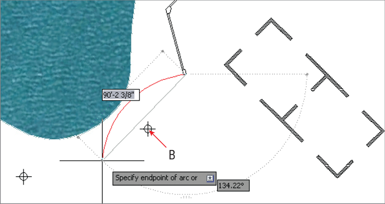
3. Toggle off Ortho mode if it is on. Observe that the arc you are drawing may curve the wrong way, against the curvature of the lake (see
Figure 5-2). The command prompt reads:
Specify endpoint of arc or
[Angle Center Direction Halfwidth Line
Radius Second pt Undo Width]:
4. Type
S (for Second Point), shown as B in
Figure 5-2, and press Enter. Normally, polyline arcs are defined by two points, and by using the second point option, you are choosing the arc to be formed by three points so that you can determine its direction of curvature.
5. Right-click the Object Snap toggle in the status bar and select Node. By turning on Node running object snap, you will be able to snap arcs to all the point objects surrounding the lake. Turn on Endpoint running object snap if it is not already on. Click B as shown in
Figure 5-2.
The point objects in the sample file are meant to guide you in the exercise. Points typically aren’t necessary when drawing curves on your own.
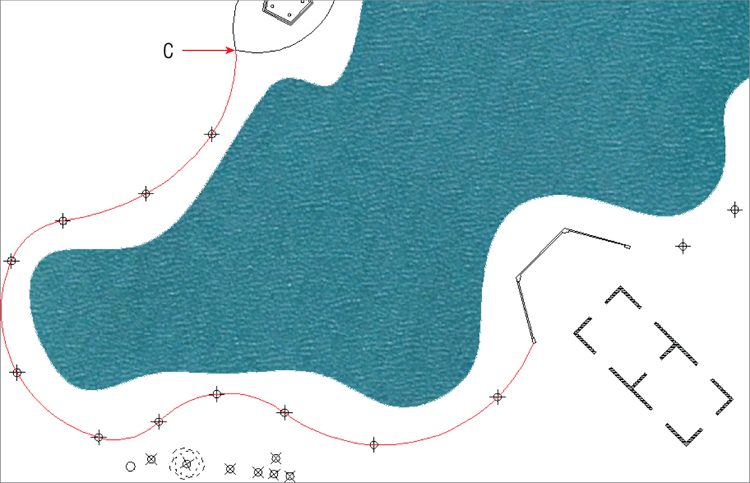
6. Click each subsequent node around the left half of the lake until you reach point C in
Figure 5-3. Press Enter to end the
PLINE command.
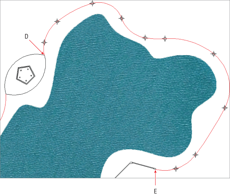
7. Press the spacebar to repeat the last command. Click point D shown in
Figure 5-4, type
A (for Arc), and press Enter.
8. Type S (for Second Point), press Enter, and snap to the node adjacent to point D.
9. Click each subsequent node around the right side of the lake until you reach point E in
Figure 5-4. Press Enter.
10. Type O (for Offset), and press Enter. Type 6 (or 2 m), and press Enter. Click the left polyline you drew around the lake in steps 1–6, and then click a point on the side of the polyline away from the lake. Click the right polyline, and click outside the lake. Click the outer arc surrounding the pentagonal structure, and then click outside the lake.
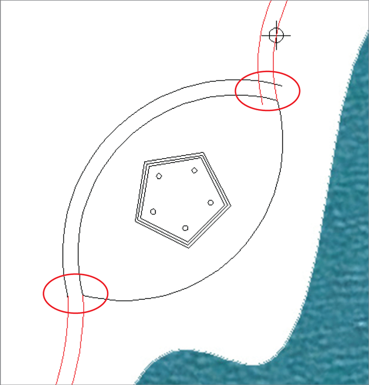
11. Click the Trim tool in the Modify panel. Press Enter to select all objects as potential cutting edges, and click the portions of the arcs that overlap in the top highlighted area in
Figure 5-5. Zoom into the lower highlighted area, and trim the arcs so that they meet at their endpoints. Press Esc to end the
TRIM command.
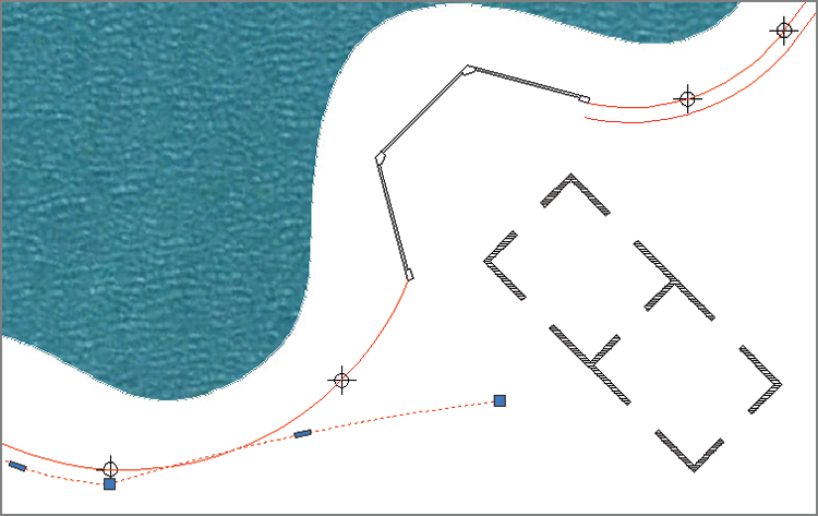
12. Pan over to the building at the bottom of the lake. We’d like the ends of the paths to open up to the building. Click the lower-left polyline to select it. Click the endpoint grip, move it down a short distance, and click again (see
Figure 5-6). You can’t get the end of the path to open up without distorting the path farther up because it’s all part of the same arc segment.
13. Press Esc, and then click the Undo button in the Quick Access toolbar.
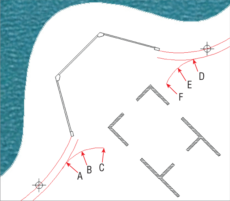
14. Click the Arc tool in the Draw panel, hold Shift down and right-click, and choose Nearest from the context menu. Click points A, B, and C in
Figure 5-7 to shape the arc as shown.
15. Press Enter twice to end, and restart the
ARC command. Type
NEA (for Nearest), press Enter, and click points D, E, and F in
Figure 5-7.
16. Zoom in and trim away the portions of the original polylines that extend beyond the new arcs you’ve just drawn.
17. Type
J (for Join), and press Enter. Select all five objects that comprise the outer path (three arcs and two polylines). Press Enter, and the command line reads:
13 segments joined into 1 polyline
There are 13 segments if you include all the arcs that make up the two polylines. You are left with a single polyline marking the outer edge of the path.
18. Press the spacebar to repeat the
JOIN command. Select the three objects along the inner edge of the path, which include two polylines and the arc above the pentagon. Press Enter, and multiple segments are joined into one polyline (see
Figure 5-8).
Use
JOIN to connect collinear lines even if there is a gap between them.
JOIN is the antidote to
BREAK.
Should You Use JOIN or PEDIT?
In previous versions of AutoCAD, objects first had to be converted into polylines and then joined using the polyline editing command called PEDIT. The streamlined JOIN command makes the older workflow unnecessary. Use it on lines, 2D and 3D polylines, arcs, elliptical arcs (sections of ellipses), and/or helices. Multiple object types can be joined at once. The resulting object type depends on what was selected.
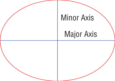
Drawing Ellipses
AutoCAD can draw perfect ovals, which are mathematically known as ellipses. Instead of stretching a cord from two pins to a moving pencil point (which is how you draw an ellipse by hand), in AutoCAD you specify the lengths of its major and minor axes (see Figure 5-9).
In this exercise, you will draw an ellipse and distribute shrubs along its edge:
1. Zoom into the area in the lower left where the remaining point objects are located.
2. Type REGEN (for Regenerate), and press Enter. The size of point objects is recalculated when the drawing is regenerated.
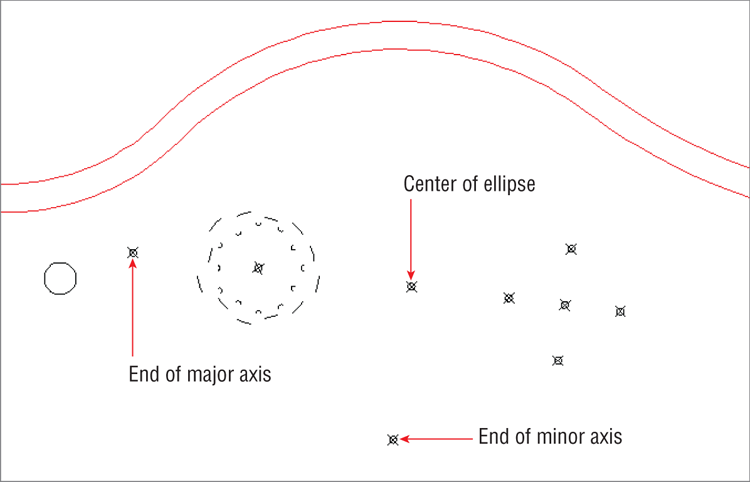
3. Open the Ellipse menu in the Draw panel, and choose the Center method. Click the center point, the end of the major axis, and the end of the minor axis, as shown in
Figure 5-10.
4. Type
BR (for Break), press Enter, and select the ellipse. The command prompt reads:
Specify second break point or [First point]:
Type F (for First Point), and press Enter.
5. Right-click the Object Snap toggle in the status bar, and select Quadrant from the context menu. Click the quadrant point (north, south, east, or west points of any circle) opposite the point object marking the end of the major axis (see
Figure 5-10), and then click the aforementioned point object itself to break the ellipse in half. The lower half of the ellipse remains, leaving an
elliptical arc.
Breaking an ellipse, arc, or circle works in a counterclockwise fashion.
6. Type
DIV (for Divide), and press Enter. Select the elliptical arc, and press Enter. The command prompt reads:
Enter the number of segments or [Block]:
Type B (for Block), and press Enter. You’ll learn more about blocks in Chapter 7, “Organizing Objects.”
7. A block called Shrub is predefined, so at the next command prompt:
Enter name of block to insert:
type Shrub, and press Enter.
8. Press Enter to accept the default when asked if you want to align the block with the selected object. (It doesn’t matter in this case because the Shrub block is a circle.)
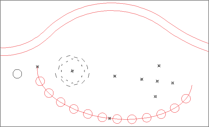
9. Type
13 (for the number of segments), and press Enter. The
DIVIDE command always creates one less point or block than the number of segments into which the object is divided. Twelve “shrubs” appear along the elliptical arc (see
Figure 5-11).
10. Delete the three points used in drawing the ellipse, the elliptical arc itself, and the black circle, which is the original Shrub block. You deleted the layout geometry and are now left with precisely positioned shrubs.
Drawing and Editing Splines
Splines are the equivalent of a French curve in traditional drafting, used for making curves of constantly changing radii. Splines have been part of AutoCAD for many releases, but the SPLINE command was completely overhauled in AutoCAD 2011. The new splines in AutoCAD are NURBS-based curves (the same type used in Autodesk® Alias® Design Surface, Maya, 3ds Max, and many other high-end 3D programs). There are two types of NURBS curves:
- Those defined by control vertices (CVs), which don’t lie on the curve except at its start and endpoints
- Those defined by fit points, which lie on the curve itself
You have more control over shaping curves with CVs, but if you want the curve to pass through specific points, or want the curve to have sharp kinks, then Fit Points mode is preferable. Fortunately, it is easy to switch between CVs and Fit Points editing modes, so you can make up your mind about which method to use to suit the situation.
Working with Control Vertices
CVs offer the most flexibility in terms of precisely shaping NURBS curves. A control frame connects CVs and represents the maximum possible curvature between adjacent CVs. You will now draw a CV spline around the lake:
1. Toggle off Object Snap, Ortho, and Polar Tracking modes on the status bar if any of them are on. Type
SPL (for Spline), and press Enter. The command prompt reads:
Current settings: Method=Fit   Knots=Chord
Specify first point or [Method Knots Object]:
Type M (for Method), and press Enter.
2. The command prompt reads:
Enter spline creation method [Fit CV] <Fit>:
Type CV (for Control Vertices), and press Enter. Click the first point anywhere along the edge of the lake.
3. Continue clicking points all the way around the lake. When you get close to the first point, type
C (for Close) and press Enter. Click the spline you just drew to reveal its CVs (see
Figure 5-12).
CV curves are typically roughed-in initially and then are refined in shape immediately afterward.
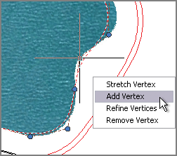
4. Position the cursor over a CV, and observe the multifunction grip menu. Select Stretch Vertex, move the cursor, and click to relocate that particular CV.
5. Try adding and removing vertices using the corresponding choices on the multifunction grip menu (see
Figure 5-13).
6. Refining a vertex transforms one vertex into two adjacent vertices. Try refining vertices in areas where the curvature is changing rapidly.
7. Another way to affect the shape of a spline is to adjust the weights of individual CVs. Double-click the spline itself (rather than a CV or the control frame) to invoke the
SPLINEDIT command. The prompt reads:
Enter an option [Open Fit data Edit vertex convert to Polyline
Reverse Undo eXit] <eXit>:
Type E (for Edit Vertex), and press Enter.
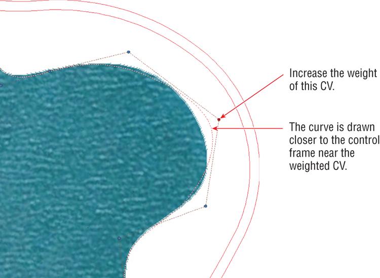
Vertices with higher weights pull the curve toward the control frame and vertices with weights below 1 (but above 0) push the spline farther away.
8. The prompt now reads:
Enter a vertex editing option [Add Delete Elevate order
Move Weight eXit] <eXit>:
Type W (for Weight), and press Enter.
9. Before entering a weight value, you must select the vertex in which you’re interested. Zoom out until you can see all the vertices, locate the red one, press Enter repeatedly to choose the default option (Next), and move the red CV one position at a time until your chosen CV turns red.
10. Type
2, and press Enter (see
Figure 5-14). The spline will get closer to the red CV and its control frame. Type
.5, and press Enter again; the curve moves farther away from the control frame. Type a value appropriate to your particular situation, and press Enter. We set a weight of 0.75 for the CV shown in
Figure 5-14 to push it away from the control frame and more closely match the shape of the lake. The weights you need to enter depend entirely on exactly where you placed the CVs when creating the curve in step 2.
11. Type X (for Exit), and press Enter. Press X and Enter twice more to exit SPLINEDIT fully.
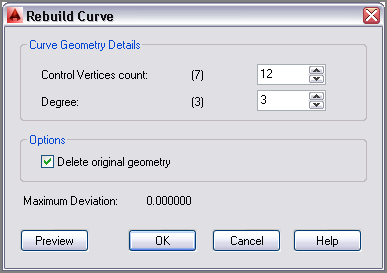
Sketch and Rebuild CVs
Instead of stretching, adding, removing, refining, and/or adjusting CVs, you can sketch spline curves freehand. The SKETCH command is admittedly difficult to use with a mouse, so if you have a stylus and a drawing tablet, try using them for a more natural drawing feel. Unfortunately, sketching splines usually results in an uneven distribution of CVs, but this can be rectified by using CVREBUILD. For an alternative natural drawing technique, draw splines on a tablet with SKETCH (using SPLINE in its type option) and then redistribute the resulting CVs with CVREBUILD. The CVREBUILD command’s Rebuild Curve dialog box is shown here:
12. Continue adjusting the spline until it closely matches the outline of the lake.
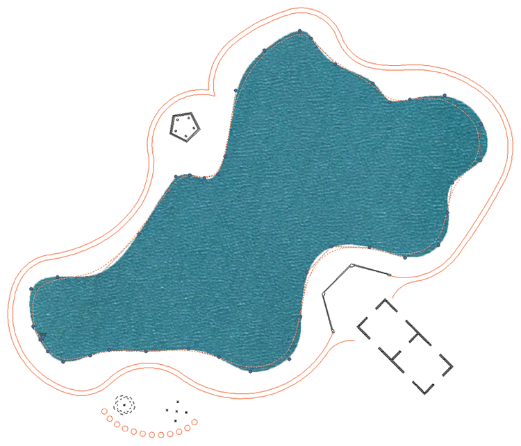
13. Type IM (for Image), and press Enter. The External References palette appears. (You’ll learn more about this palette in Chapter 9, “Working with Blocks and Xrefs.”) The lake that you have been tracing is an image that you will now detach.
14. Right-click Pond in the External References palette, and choose Detach Image. Close the External References palette. Select the pond spline, and change its color to Blue in the Properties panel (see
Figure 5-15). The pond is now represented by a blue curve rather than a blue image.
Working with Fit Points
Fit point splines are straightforward in the sense that the fit points you click lie on (or very close to) the curve itself. Controlling the shape of a fit curve on the most basic level is a matter of adding more fit points in strategic locations. There are a few advanced options affecting the shape of a spline in between fit points (Tangent, Tolerance, Kink, and Knot Parameterization), and you will use Kink in this exercise to establish sharp points on the spline.
1. Zoom into the area at the bottom of the lake where you distributed the shrubs earlier in this chapter in an elliptical arc. More specifically, zoom into the grouping of five points. Type REGEN, and press Enter to regenerate the display and thus automatically resize the point objects.
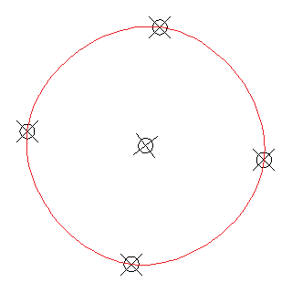
2. Expand the Draw panel, and click the Spline Fit tool at the top left. Toggle on Object Snap mode in the status bar (with Node snap on), and click the top point, the point on the right, the bottom, and then the one on the left. Type
C (for Close), and press Enter. The fit curve looks very much like a circle, although it is not perfectly round (see
Figure 5-16). This will be the start of an abstract tree representation.
3. Toggle on Dynamic Input on the status bar. Select the spline you just drew, type SPLINEDIT, and press Enter. Choose Fit Data from the dynamic input menu. Then choose Add from the next dynamic input menu that appears.
4. The prompt reads:
Specify existing fit point on spline <exit>:
Click the top point.
5. The prompt now says:
Specify new fit point to add <exit>:
This particular command requires that you snap the new fit point, so type NEA (for Nearest) and press Enter. Click the curve in between the top and right points. Press Enter four times to exit SPLINEDIT fully.

6. Another way to add fit points is with the multifunction grips, although this method doesn’t work on the first point. To use this feature, click the spline to select it, hover the cursor over the right point, and choose Add Fit Point from the menu that appears. Hold Shift, right-click, and choose Nearest from the context menu. Click a point between the right and bottom points.
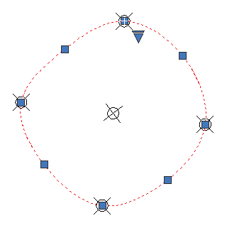
7. Repeat the previous step twice more, adding additional fit points between the bottom, left, and top points (see
Figure 5-17).
8. Double-click the spline itself to invoke the
SPLINEDIT command without typing. Type
F (for Fit Data), and press Enter. The prompt reads:
Enter a fit data option
[Add Open Delete Kink Move Purge Tangents
toLerance eXit] <eXit>:
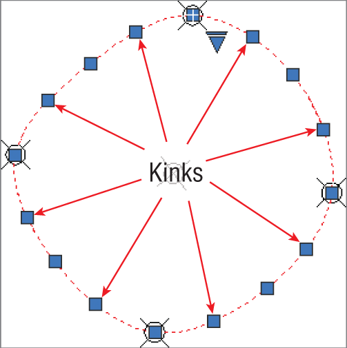
Type
K (for Kink), and click eight points in between all the existing fit points (see
Figure 5-18). Press Enter three times to exit the command fully.
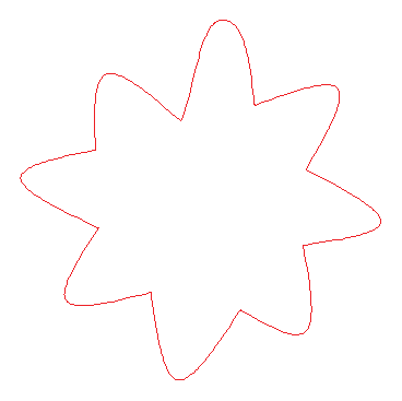
9. Click each kink grip, and move it in toward the center to create an abstract representation of a tree. Delete the five point objects that helped you lay out the tree (see
Figure 5-19). If you have trouble selecting point objects, try changing their size with the
DDPTYPE and
REGEN commands.
Blending Between Objects with Splines
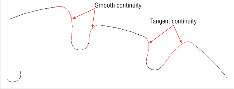
The BLEND command creates a CV spline in between two selected lines, circular or elliptical arcs, splines, or any combination of these object types. Blend curves join the endpoints of the two objects with a curve having either tangent or smooth continuity. There is a subtle difference between these types of blending.
A blend curve with tangent continuity has its control frame parallel to the control frame of the adjacent curve. A blend curve with curvature continuity not only has its control frame parallel to the control frame of the adjacent curve, but the control frames have equal lengths. In simpler terms, tangent continuity is smooth, and smooth continuity is “perfectly smooth.” In the following steps, you will create blend curves with two types of curvature:
1. Pan over to the other “tree” to the left of the tree you’ve drawn with kinks. Type BLEND, and press Enter.
2. The prompt reads:
Continuity = Tangent
Select first object or [CONtinuity]:
Select a flat arc and a tight arc, and the command is finished. A CV spline with tangent continuity blends between the two arcs.
3. Press the spacebar to repeat
BLEND, type
CON (for Continuity), press Enter, type
S (for Smooth), and press Enter again. Click two adjacent arcs to create another blend curve (see
Figure 5-20).
4. Continue blending all the adjacent curves in the tree. Delete the point object at the center.
Figure 5-21 shows the completed drawing.
5. Your drawing should now resemble Ch5-B.dwg (or Ch5-B-metric.dwg), which is available at this book’s web page.
The Essentials and Beyond
You have learned how to shape many types of curvilinear objects in this chapter, including circular and elliptical arcs, polylines, ellipses, and CV and fit point NURBS-based splines. You’ve broken and joined objects, and blended smoothly between adjacent curves. In short, you now have the skills to shape just about any curve you can imagine with a fine degree of precision, which is what AutoCAD is all about.
Additional Exercise
- Explore the HELIX command on your own. The HELIX command creates spirals and helices. You are welcome to stick with two dimensions for now and create spirals with this command. When you learn how to navigate and model in 3D (in Chapters 16 and 17), you can use this command to create springs, screw threads, or even DNA.