5

Leveraging Points, Lines, and Curves

Now that we understand the basic tools and methods of Civil 3D, this chapter will dive into the application and intersection of these tools to better develop a confident infrastructure design. Civil 3D is a dynamic program with not only intelligent components and design processes but also integrated workflows that adjust when dependent parts of the design adjust or change, which results in less time spent recreating work or formatting when work is updated automatically.

In Chapter 4, Configuring Survey Data with Civil 3D, we reviewed many of the preparational tasks required to be performed in our Survey Model. In the previous chapter, we were afforded what I would consider a lay-up in the sense that survey data has already been converted into the 2D and 3D geometry making up our Survey Model.

Occasionally, we will come across instances where specific components will be resurveyed and then provided to the designer after the initial composition of the Survey Model in the form of an ASCII file, which is essentially a text-based file with survey points including point numbers, northings, eastings, elevations, and descriptions, also seen abbreviated as PNEZD or some similar variation.

With that, the following key topics will be covered in this chapter:

• Setting up a new file to import points from survey data
• Introduction to points
• Introduction to lines and curves

Throughout this chapter, we’ll incorporate various point/line/curve commands to get an idea of how we can import survey and supplemental data relatively easily and convert it into geometry that can be incorporated into our overall Survey Model.

For this example, we’re going to start with a brand-new file using the Civil 3D template we created in Chapter 4, Configuring Survey Data with Civil 3D, and use the ASCII file, both of which can be found in our Practical Autodesk Civil 3D 2024Chapter 5 subfolders entitled Company Template File.dwt and Survey Model.asc, respectively.

Technical requirements

The exercise files for this chapter are available at https://packt.link/UoiPn

Setting up a new file to import points from survey data

To kick things off, let’s go ahead and create a new drawing using our new Project/Company drawing template file that we created, which can be found in our Practical Autodesk Civil 3D 2024Chapter 5 subfolder.

We’ll open Menu Browser in the top-left corner of our Civil 3D session, and then select New | Drawing, as shown in Figure 5.1:

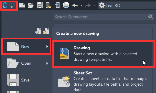
Figure 5.1 – Create a new drawing with a specified template

Once selected, we’ll be asked to select the drawing template that we wish to create a drawing from, at which point, we’ll navigate to our Practical Autodesk Civil 3D 2024Chapter 5 location, select the Company Template File.dwt file, and click Open (refer to Figure 5.2):

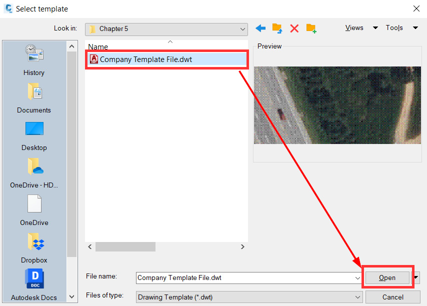
Figure 5.2 – Select drawing template

After selecting the file and clicking Open, a new drawing will be created that already incorporates the styles and settings that were applied to our Survey Model in Chapter 4, Configuring Survey Data with Civil 3D, prior to clicking Save As to create our drawing template. You’ll notice right off the bat that our new drawing has been created to include Aerial Imagery as a background provided through the Geolocation ribbon.

This is due to the fact that when we saved our file as a drawing template, we saved the coordinate system projection as well. We can confirm this again by selecting the Settings tab in Prospector by right-clicking on our filename and selecting Edit Drawing Settings… to pull up the Drawing Settings dialog box that has the projection identified, as shown in Figure 5.3:

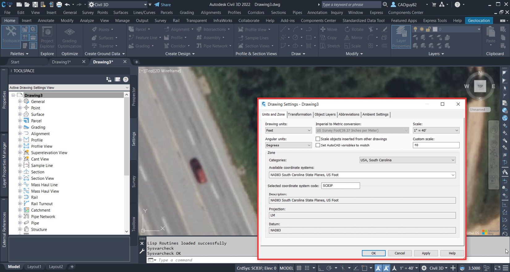
Figure 5.3 – The Drawing Settings dialog box

That said, if you tend to work on projects in multiple states, you can either update the setting so as not to include a coordinate system projection or begin to think about ways you can create multiple drawing templates for each state in which you will be performing the design. Either way, a few key things to think about when it comes to creating drawing templates include the following:

• We want to make sure that we have a great foundation to build off whenever we create new drawings and start new projects
• Make starting new drawings and projects as streamlined and automated as possible to ensure that the majority of time spent is on actual design and production
• Drive consistency through efficiency in all of your projects and designs

Once we’re comfortable with the direction we’re headed with the new drawing, and all the styles, settings, and our coordinate system assignment, let’s go ahead and save our newly created drawing. To do so, we’ll head back up to Menu Browser, hover over Save As, and select Drawing, as shown in Figure 5.4:

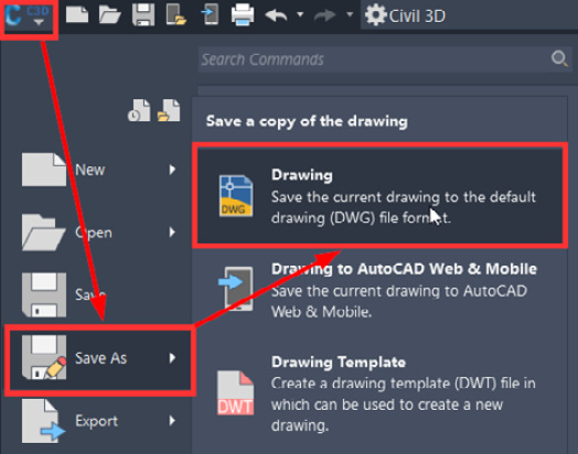
Figure 5.4 – Save our new drawing

Once selected, we’ll be presented with a Save Drawing As dialog box, at which point we’ll navigate to our Practical Autodesk Civil 3D 2024Chapter 5 location, call the Survey Model.dwg file, and click on the Save button, as shown in Figure 5.5:

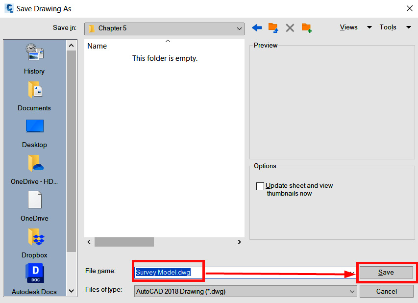
Figure 5.5 – Save our new drawing

Now that we have our file set up and saved, we can next move on to understanding how we can incorporate survey data via ASCII point files into our Survey Model for future use.

Introduction to points

Points in Civil 3D can have many different applications, purposes, and nomenclature. They are often viewed as one of the most basic foundational components that can be used for the creation of models and design progression and for painting the story of our overall design.

For the purposes of this chapter, we’ll focus on the importing process of points generated from our surveyed data, and identify some beneficial applications where these imported points can be processed to generate geometry and models to be displayed in our Survey Model.dwg file.

Starting with the importing process, we’ll be able to access the import Points command by going up to the ribbon, selecting the Insert tab, and then selecting the Points from File tool, as shown in Figure 5.6:

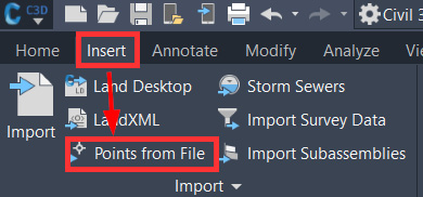
Figure 5.6 – Import points from file

Once selected, we’ll be presented with the Import Points dialog box where we’ll go ahead and import the Survey Model ASCII file into our Survey Model.dwg file using the following steps, as numbered in Figure 5.7:

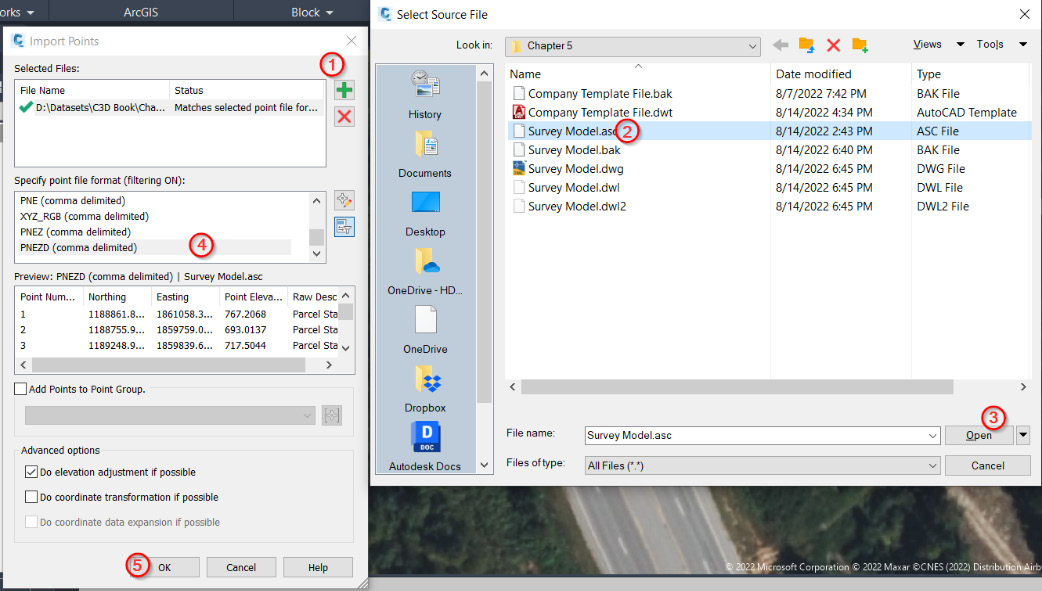
Figure 5.7 – The Import Points dialog box

1. Click on the Add Files icon.
2. Select the Survey Model.asc file located in Practical Autodesk Civil 3D 2024Chapter 5.
3. Click the Open button.
4. Select PNEZD as the point file format (PNEZD represents Point Number, Northing, Easting, Elevation, Z Value/Elevation, and Description).
5. Click the OK button.

Note

Importing may take a little while in this instance as there are 36,294 points to import from the Survey Model.asc file. Civil 3D can accept a variety of point files such as .txt, .csv, and more. It can also accept them in a few different formats such as comma-delineated or space-delineated, depending on how the point file was created in the field.

After all our points have been imported, we not only see them displayed in our model space but also listed in our panorama if we select Points in TOOLSPACE | Prospector, as shown in Figure 5.8:

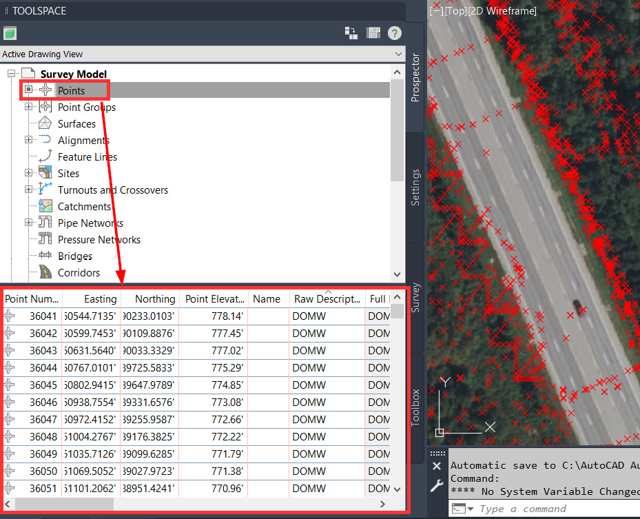
Figure 5.8 – Points displayed in the panorama

If you were to navigate through the panorama, you would notice that each of the points had a raw and full description associated with them as well. By using these descriptions, we can start to organize and add filterable selections by parsing our points out and generating individual point groups based on the descriptions.

It is important to note that the points imported here are referred to as coordinate geometry (COGO) points. These points are more directly editable than other points in Civil 3D such as survey points, which are linked directly to a survey database and are more difficult to adjust if need be.

With that, let’s go ahead and click the + icon next to Point Groups to expand it out a bit. We notice that there is currently a point group already available labeled _All Points. It is important to note that the _All Points point group is included by default and cannot be deleted from our drawings. On the flip side, any new point groups that are created can be deleted as needed.

In any event, let’s go ahead and add a few organizational levels to our points in our current file. To do so, we’ll right-click on Point Groups in Prospector and select New..., as shown in Figure 5.9:

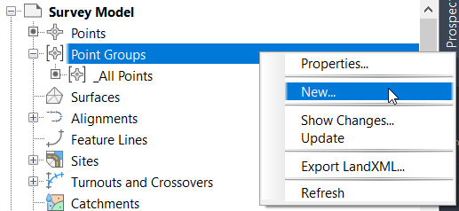
Figure 5.9 – Create new point group

Once selected, we’ll be presented with the Point Group Properties dialog box where we can begin to further define and organize the points that we inserted into our file. In the Information tab, let’s go ahead and give our first point group a proper name, description, and default point and label styles as listed next, and shown in Figure 5.10:

• Name: Ground
• Description: Existing Ground Survey Shots
• Default Point Style: <none>
• Default Point Label Style: <none>

It is important to note that the <none> point style and point label style will assure us that these points are not displayed in our view. However, we can still use these to generate our 2D and 3D geometry moving forward.

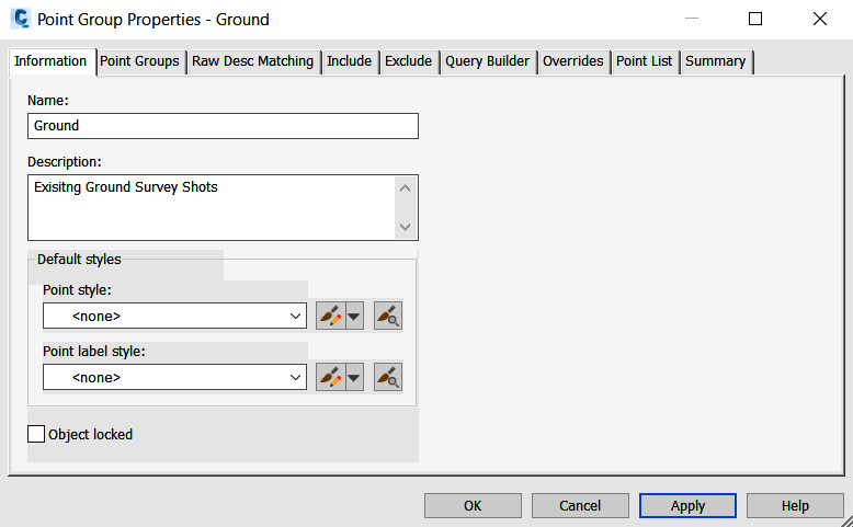
Figure 5.10 – Point Group Properties information tab

Next, we’ll switch over to the Include tab, check the box next to With raw descriptions matching, and type *GRND* into the field next to this option, as shown in Figure 5.11. The * symbol is used as a wildcard to match and include any points that contain GRND in the raw description of the points currently residing in the file:

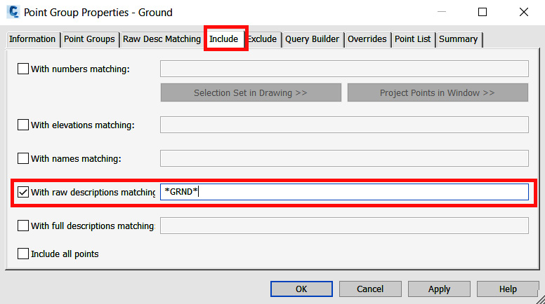
Figure 5.11 – Point Group Properties – With raw descriptions matching

Now, if we switch over to the Point List tab and click on the Apply button in the lower right, we’ll see a fully comprehensive list of all the points in our file that include GRND in the raw description, as shown in Figure 5.12:

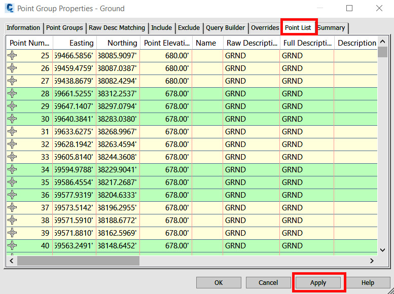
Figure 5.12 – Point Group Properties – Point List

Next, we’ll move on to our Sanitary Sewer Manhole points. As we did during the first point group creation, we’ll right-click on Point Groups, and select New again. In the Information tab of the Point Group Properties dialog box, we’ll go ahead and fill out the Name (Sanitary Sewer Manholes) and Description (Existing Sanitary Sewer Manholes) fields.

We’ll select Sanitary Sewer Manhole as Point style and then apply <none> as Point label style, as shown in Figure 5.13:

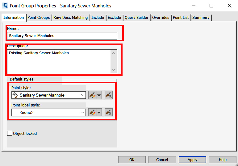
Figure 5.13 – Point Group Properties – Sanitary Sewer Manholes point group

Moving over to the Include tab, we’ll want to check the box next to With raw description matching and type *SSWR* into the field next to this option, and then click on the Apply and OK buttons.

For Storm Drainage, we’ll take a slightly different approach by going into the Point Groups section in Prospector, right-clicking on our Sanitary Sewer Manholes point group that we just created, and selecting Copy..., as shown in Figure 5.14:

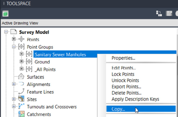
Figure 5.14 – Copy point group

You’ll notice that a new point group called Copy of Sanitary Sewer Manholes is now displayed in our list of point groups. To update and change this to apply to Storm Drainage Structures, we’ll go ahead and right-click on the copied point group and select Properties..., as shown in Figure 5.15:

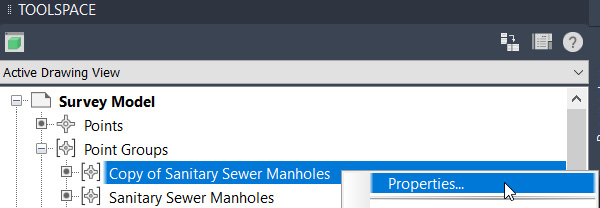
Figure 5.15 – Edit point group properties

In the Information tab, we’ll go ahead and fill out the Name and Description fields and apply default styles, as shown in Figure 5.16:

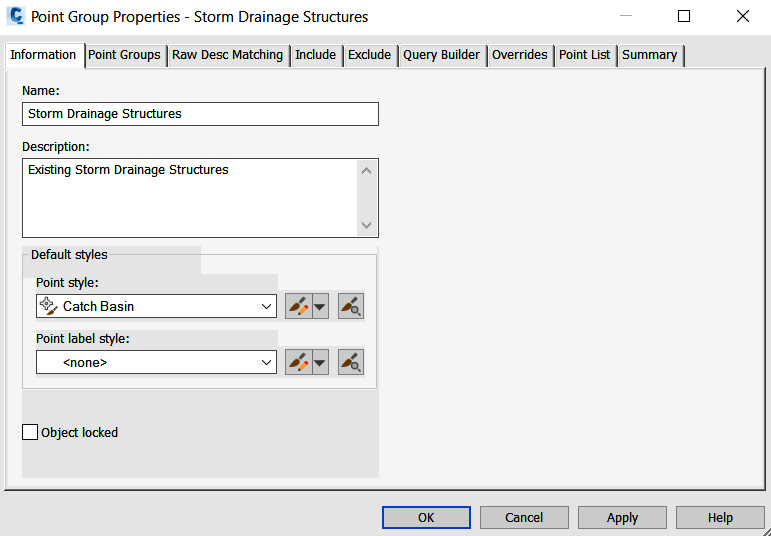
Figure 5.16 – Point Group Properties – Storm Drainage Structures

Then, we’ll switch over to the Include tab and change With raw description matching from *SSWR* to *STRM* in the field next to this option, and then click on the Apply and OK buttons.

Finally, using the steps outlined throughout this section, let’s go ahead and create three more point groups to cover Domestic Water Pipeline, Parcel Staking, and York Hwy CL. For the Domestic Water Pipeline and the York Hwy CL point groups, we’ll apply the <none> point style and point label style. For the Parcel Staking point group, we’ll want to apply the Iron Pin Point style.

In the end, we should only see Sanitary Sewer Manholes and Storm Drainage Structures in the model space in our file, as shown in Figure 5.17. It is important to note that we can control the appearance of points with point groups as well as point styles.

This itself can be strategically used further in design and labeling, but be sure to understand there is still a control hierarchy where point groups are the parent display controlling how all points contained within are set, and then individual point styles themselves will apply to those not within point groups.

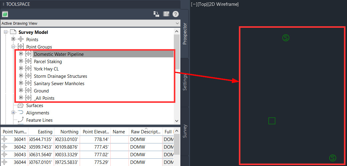
Figure 5.17 – Final display after point groups are created

Although it may not seem like much based on what we can currently see in our model space, we have actually done a tremendous service by setting ourselves up to leverage some additional tools available to us within Civil 3D to streamline the generation of a full survey display. These tools and workflows will be discussed throughout the remainder of this chapter.

Introduction to lines and curves

Now that we have our points imported into our file, we can start to think about ways to leverage the line and curve commands to generate some of our basic survey geometry. In the previous section, we created several point groups in an effort to organize the survey data that we received and imported into our Survey Model.

In our first exercise, we’ll go ahead and convert the existing road centerline points into real linework. With that, let’s go ahead and identify the point number range within the York Hwy CL point group (these points are meant to depict the centerline of York Highway).

To identify the point range, we’ll go back into our TOOLSPACE | Prospector tab, select the point group labeled York Hwy CL, and take note of the point numbers in the panorama listed, as shown in Figure 5.18:

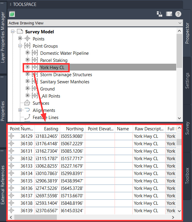
Figure 5.18 – York Hwy CL point group list

We’ll notice that the point numbers start with #36,083 and end with #36,294.

Let’s now move over to the Home ribbon, zoom to the Draw panel, and select the down arrow next to the Line icon to display all the available options we have to generate lines, as shown in Figure 5.19:

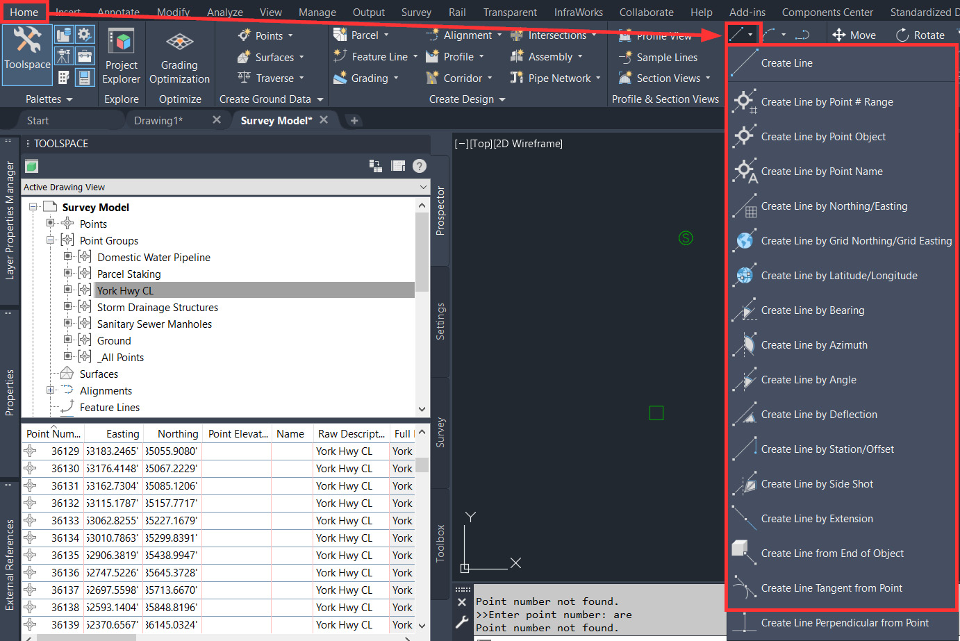
Figure 5.19 – Create a line

As you can see, this list is quite extensive and provides a multitude of ways for us to generate lines in our current file. For additional details about each method, we can simply hover our mouse over each method, at which point a detailed overview will be displayed explaining how each can be applied.

For the purposes of this exercise, let’s focus on those methods that allow us to incorporate points into our line generation:

• Create Line by Point # Range: We can generate lines by inputting the range of points that we’d like to connect between
• Create Line by Point Object: We can generate lines by selecting the points that we’d like to connect between
• Create Line by Point Name: We can generate lines by inputting the point name associated with the points we’d like to connect between

In our case, since we do not have a point name applied to our points, and we have already set our York Hwy CL point group display to <none>, we are left to use the Create Line by Point # Range command.

Let’s go ahead and select that command in our Home | Draw | Lines pull-down menu. We’ll notice at the very bottom of our session that we will be asked to enter the point number. Instead of typing in 104 point numbers manually, we can simply type in the point range that we took note of earlier, for instance, we’re using a point range of 35217-35321 (as shown in Figure 5.20) and then hit the Enter key on the keyboard:

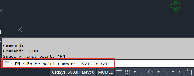
Figure 5.20 – Enter point numbers at the command line

Once the command has been processed, we’ll use the following steps to convert our new linework into a polyline (refer to Figure 5.21):

1. Zoom out to the point where we have all the new linework within our view in the model space.
2. Go to the Modify ribbon.
3. Go to the Modify panel.
4. Click the down arrow in the Modify panel to expand the tools.
5. Select the Join command to convert individual lines into one continuous 3D polyline.
6. Select all lines.
7. Hit the Enter key on the keyboard:

Figure 5.21 – Join lines to create a polyline

Next, we’ll use the following steps to place our newly created polyline on the correct survey layer (refer to Figure 5.22):

1. Select the polyline we just created.
2. Go to the Home ribbon.
3. Go to the Layers panel.
4. Select the down arrow next to the current layer name.
5. Scroll down and select the V-ROAD-CNTR layer:

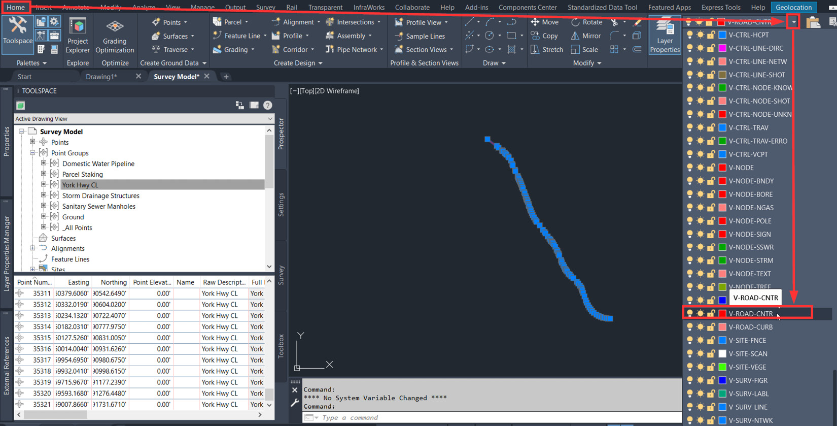
Figure 5.22 – Place polyline on corresponding layer

We have now officially converted our first set of points into geometry within our Survey Model. By converting our data into actual geometry, we are building the existing conditions, or built environment, from which we will be able to generate our design.

Let’s continue to proceed with converting our utility point groups using the same workflow and then place them on their corresponding layers as follows:

• Storm Drainage Structures:
  • Using point range 35,163-35,174
  • Use the Join command to create one continuous 3D polyline
  • Place the resulting linework on the V-STRM-MAIN layer
• Sanitary Sewer Manholes:
  • Using point range 35,175-35,193
  • Use the Join command to create one continuous 3D polyline
  • Place the resulting linework on the V-SSWR-MAIN layer
• Domestic Water Pipeline:
  • Using point range 35,194-35,215
  • Use the Join command to create one continuous 3D polyline
  • Place the resulting linework on the V-WATR-MAIN layer

Moving on to our Parcel Staking point group, we’ll use the Create Line by Point Object command (refer to Figure 5.23). Using this command, we will be prompted to select a start point and an end point.

Once selected, a line will be automatically generated to connect the start and end points. Before starting this command, we’ll want to set our current layer to V-PROP-LINE so that all the new linework we create during this process will be created on the correct layer:

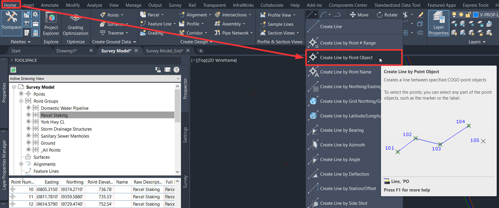
Figure 5.23 – Create Line by Point Object

Starting with the southern parcel, we’ll select points to generate our parcel boundary, as shown in Figure 5.24:

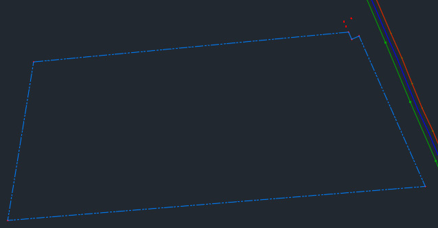
Figure 5.24 – Existing parcel (southern)

Next, we’ll perform the same task on our northern parcel, with the finished result shown in Figure 5.25:

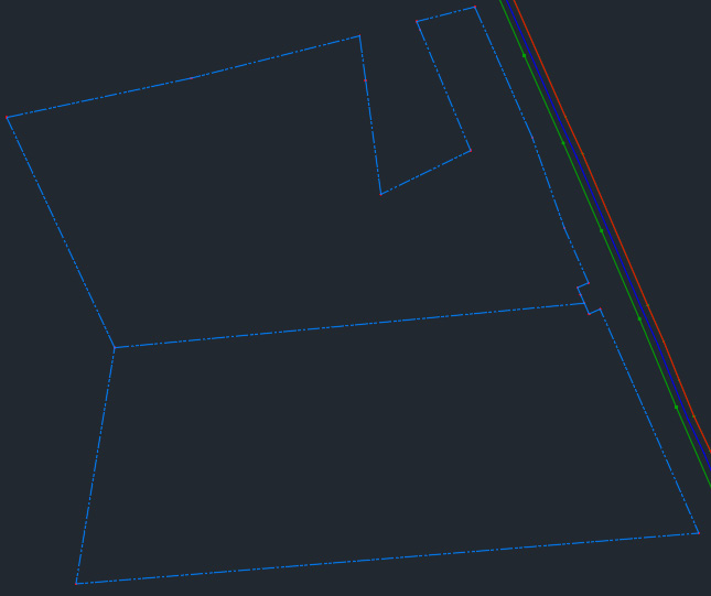
Figure 5.25 – Existing parcels

With the exception of the Ground point group, we have now converted all remaining point groups into real geometry within our Survey Model depicting various components of the existing built environment.

As I’m sure you’ve noticed, we have placed a heavy emphasis on the line commands as we are able to use these commands in conjunction with our surveyed points to generate our linework. The curve commands can be accessed within the Home ribbon in the Draw panel, similar to the line commands, as shown in Figure 5.26:

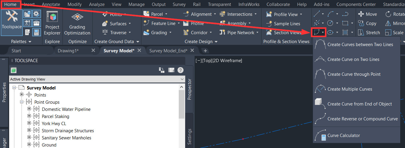
Figure 5.26 – Curve commands

As displayed in Figure 5.26, we do not have the ability to generate curves from our point groups automatically, but we do have the ability to create curves:

• Create Curve between Two Lines: Allows us to add a fillet to two selected lines
• Create Curve on Two Lines: Adds a fillet but leaves the selected lines untouched
• Create Curve through Point: Creates a fillet by selecting lines and defining the location for the curve to run through
• Create Multiple Curves: Creates multiple compound curves between selected lines with varying lengths and radii
• Create Curve from End of Object: Creates an arc as a continuation of the selected line
• Create Reverse or Compound Curve: Creates either a reverse or compound curve as a continuation of the selected arc

Although we do not currently have a workflow identified where these commands can be utilized, we will be revisiting these tools and applying them in workflows identified in Chapter 7, Alignments - The Second Foundational Component to Designs within Civil 3D, and Chapter 10, Roadway Modeling Tool Belt for Everyday Use.

Summary

We are now well on our way to fully understanding how we can set up a Survey Model and establish a solid foundation from which we can build our design. In the event that the surveyor is required to go out into the field to survey additional data, we have a good understanding and should feel a little more at ease if we are to add additional survey data and convert linework to be displayed in our Survey Model.

In our next few chapters, we’ll continue to build up our Survey Model to incorporate 3D elements for which we can data-reference as needed and develop our design models. In the next chapter, in particular, we’ll use the Ground point group that we left untouched to understand how we can build, manage, and analyze our Surface Models.