
2
Signal Models for Modulation Classification
2.1 Introduction
Signal models are the starting point of every meaningful modulation classification strategy. Algorithms such as likelihood-based (Huang and Polydoros, 1995; Wei and Mendel, 2000; Shi and Karasawa 2012), distribution test-based (Wang and Wang, 2010; Urriza et al., 2011; Zhu, Aslam and Nandi, 2014) and feature-based classifiers (Azzouz and Nandi, 1996; Spooner, 1996; Swami and Sadler, 2000) all require an established signal model to derive the corresponding rules for classification decision making. While some unsupervised machine learning algorithms could function without a reference signal model, the optimization of such algorithms still relies on the knowledge of a known signal model. Meanwhile, as the validation of modulation classifiers are often realized by computer-aided simulation, accurate signal modelling provides meaningful scenarios for evaluating the performance of various modulation classifiers.
The objective of this chapter is to establish some unified signal models for the development of all modulation classifiers from Chapters 3 to 7, and to provide a level ground for the validation of each modulation classifier in Chapter 8. Through the process, the accuracy of the models will be the first priority as it provides credible evidence to aid the design of specific modulation classification strategies for real world applications in Chapters 9 and 10. That, however, is with a fine balance of simplicity in the models to enable theoretical analysis and to provide computationally efficient implementations.
In this chapter, mathematical models of communication signals are instituted for three popular communication channels, namely additive white Gaussian noise channel, fading channel, and non-Gaussian noise channel.
Additive white Gaussian noise is one of the most widely used noise models in many signal processing problems. It is of much relevance to the transmission of signals in both wired and wireless communication media where wideband Gaussian noises are produced by thermal vibration in conductors and radiation from various sources. The popularity of additive white Gaussian noise is evidential in most literature on modulation classification where the noise model is considered the fundamental limitation to accurate modulation classification.
Fading channel is largely concerned with wireless communication, where signals are received as delayed and attenuated copies after being absorbed, reflected and diffracted by different objects. Fading, especially deep fading, drastically changes the property of the transmitted signal and imposes a tough challenge on the robustness of a modulation classifier. Though early literature on modulation classifier focused on the validation of algorithms in AWGN channel, the current standard requires the robustness in fading channel as an important trait. In this chapter, a unified model of a fading channel is presented with flexible representation of different fading scenarios. It is worth noting that AWGN noise will also be considered in the fading channel as to approach a more realistic real world channel condition.
Non-Gaussian noises are often used to model impulsive noises which are a step further to model the noises in a real radio communication channel. Impulsive noise, unlike Gaussian noise, has a heavy-tailed probability density function, meaning higher probability for high power noise components. Such noises are often the result of incidental electromagnetic radiation from man-made sources. While not featured in most modulation classification literature, impulsive noises have received an increasing amount of attention in recent years. Despite the complexity in the modelling of impulsive noise, it is worth the effort to try and accommodate the signal model for a more practical approximation of the real world radio channels. In this chapter, three non-Gaussian noise models will be presented for modelling the impulsive noise. However, such noises will be considered solely without extra AWGN noise or fading effects.
2.2 Signal Model in AWGN Channel
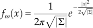
Additive white Gaussian noise is characterized with constant spectral density and a Gaussian amplitude distribution of zero mean. Giving the additive noise a complex representation ω = I(ω) + jQ(ω), the complex probability density function (PDF) of the complex noise can be found as equation (2.1), where ∑ is the covariance matrix of the complex noise, |∑| is the determinant of ∑, |x| is the Euclidean norm of the complex noise and the noise mean is zero.
Since many algorithms are interested in the in-phase and quadrature segments of the signal, it is important to derive the corresponding PDF of the in-phase and quadrature segments of the additive noise. Fortunately, when AWGN noises are projected onto any orthonormal segments the resulting projection has independent and identical Gaussian distributions. The resulting covariance matrix can be found as equation (2.2),
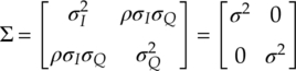
where variance for the in-phase segment ![]() and the quadrature segment
and the quadrature segment ![]() and are replaced with a shared identical variance σ2, and the correlation between two segments is zero. Thus, the desired PDFs of each segment can be easily derived as shown in equation (2.3).
and are replaced with a shared identical variance σ2, and the correlation between two segments is zero. Thus, the desired PDFs of each segment can be easily derived as shown in equation (2.3).
As suggested by the term “additive”, the AWGN noise is added to the transmitted signal to give the signal model in AWGN channel, as shown in equation (2.4).
An illustration of the received 4-QAM signal in an AWGN channel with SNR of 10 dB is given in Figure 2.1.
Figure 2.1 Constellation of 4-QAM signal in AWGN with SNR = 10 dB.
In the following subsections, the PDFs of received signals in their I-Q segments, phase and magnitude distributions are derived.
2.2.1 Signal Distribution of I-Q Segments
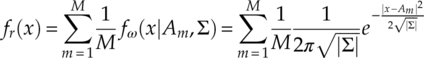
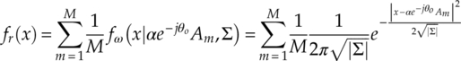
Assuming the signal modulation ![]() ; has an alphabet A of M symbols and the symbol Am having the equal probability to be transmitted, with overall distribution being considered as M number of AWGN noise distributions shifted to different modulation symbols, the complex PDF of the received signal is given by equation (2.5), where 1/M is the probability of Am being transmitted. Figure 2.2 provides an illustration of the distribution of 4-QAM signals in an AWGN channel with SNR of 10 dB on the I-Q plane.
; has an alphabet A of M symbols and the symbol Am having the equal probability to be transmitted, with overall distribution being considered as M number of AWGN noise distributions shifted to different modulation symbols, the complex PDF of the received signal is given by equation (2.5), where 1/M is the probability of Am being transmitted. Figure 2.2 provides an illustration of the distribution of 4-QAM signals in an AWGN channel with SNR of 10 dB on the I-Q plane.
Figure 2.2 PDF of 4-QAM signals in AWGN channel with SNR = 10 dB.
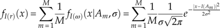
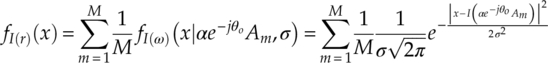
Following the same logic of the derivation of the complex PDF, the distribution of received signals on their in-phase and quadrature segments can be found by replacing the variance by half of the noise variance and the mean of the noise distribution with in-phase and quadrature segments of the modulation symbols [equation (2.6)].
An illustration of the PDF is given in Figure 2.3.
Figure 2.3 PDF of 4-QAM signals I-Q segments in AWGN channel with SNR = 10 dB.
2.2.2 Signal Distribution of Signal Phase
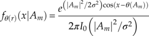
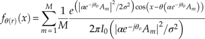
Signal phase is easily recognized as an intuitive object for analysis when the classification of PSK modulations is concerned. That is without mentioning the robustness of signal phase in channel with attenuation. According to Bennett (1956), with added noise, received signal samples from the same modulation symbol Am have a phase PDF given by equation (2.7),

where |Am| is the magnitude of the symbol Am, θ(Am) is its phase, and erf(·) is the error function. Given the complex form of the PDF, the von Mises distribution is often considered as a close approximation [equation (2.8)], where I0(·) denotes the modified Bessel function of order zero. The von Mises distribution is used primarily in this book for analytical content. However, it is worth noting that the von Mises distribution deviates from the accurate phase PDF at low SNR. Therefore, validations are provided in cases where the von Mises approximation is used.
For any modulation, the overall distribution of a received signal in AWGN channel can be found as a combination of distributions from each modulation symbol [equation (2.9)].
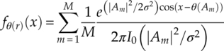
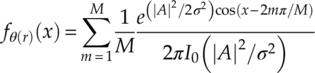
With an identical symbol magnitude |A| and the phase for symbol Am expressed as θ(Am) = 2mπ/M, the PDF of a M-PSK modulation can be found as shown in equation (2.10).
2.2.3 Signal Distribution of Signal Magnitude
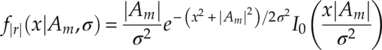
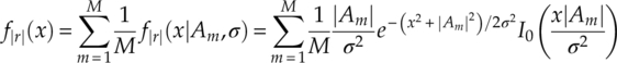
The signal magnitude has a unique feature of being robust against phase offset, frequency offset or any kind of rotational change to the transmitted signal. In this book, we approximate the PDF of the signal magnitude distribution to a Rice distribution. Given a single modulation symbol Am and AWGN noise of variance σ2, the PDF of the received signal from this single symbol can be found as shown in equation (2.11), which leads to the overall signal magnitude distribution as a sum of Rice distributions from each modulation symbol, equation (2.12).
2.3 Signal Models in Fading Channel
Instead of modelling each fading type, we characterize the joint effect of them into three categories: attenuation, phase offset and frequency offset. Depending on the nature of the fading channel, two types of fading scenarios are generally considered for signal phase offset: slow fading and fast fading. Slow fading is normally caused by shadowing (or shadow fading) when the signal is obscured by a large object from a line-of-sight communication (Goldsmith, 2005). As the coherent time of the shadow fading channel is significantly longer than the signal period, the effect of attenuation and phase offset remains constant. Therefore, a constant channel gain α and phase offset θ0 can be used to model the received signal after slow fading [equation (2.13)].
The resulting effect can be observed from a simulated 4-QAM signal in slow fading channel with channel gain at 0.5, phase offset at 10° and AWGN noise of 10 dB in Figure 2.4.
Figure 2.4 Constellation of 4-QAM signal in slow fading channel.
For the development of likelihood-based classifiers, it is useful to derive the updated signal PDFs in the slow fading channel to compensate the effect of attenuation and phase offset. As the fading channel does not modify the additive noise, only the terms related to transmitted symbols need to be changed. Given that the constant channel gain α and phase offset θ0, the transmitted symbol Am is shifted to the new position given by ![]() . The updated PDF of the complex signal after a slow fading channel can then be found by substituting the shifted symbols into equation (2.5), whence equation (2.14) is derived.
. The updated PDF of the complex signal after a slow fading channel can then be found by substituting the shifted symbols into equation (2.5), whence equation (2.14) is derived.
Similarly, the PDFs for signal I-Q segments, phase and magnitude can be derived accordingly as equations (2.15)–(2.17).

It is worth noting that while the PDF of the signal phase is much less sensitive to channel attenuation, it is much more vulnerable to phase offset. Meanwhile, the signal magnitude PDF is not affected by the phase offset at all as the PDF can be rewritten as equation (2.18).

Fast fading, caused by multipath fading where signals are reflected by objects of different properties in the radio channel, imposes a much different effect on the transmitted signal, as the coherent channel time in a fast fading channel is considered small. The effects of attenuation and phase offset vary with time. In this book, we assume that both the attenuation and phase offset are random processes with Gaussian distributions. The attenuation is given by equation (2.19),
where α(t) is the channel gain at time t, α is the mean attenuation and ![]() is the variance of the channel gain. The phase offset is given by equation (2.20), where
is the variance of the channel gain. The phase offset is given by equation (2.20), where
θo(t) is the channel gain at time t, θo is the mean attenuation and ![]() is the variance of the channel gain. Both expressions give a combined effect of slow and fast fading. When α and θo are both zero, the fading consists of only fast attenuation and fast phase offset. When
is the variance of the channel gain. Both expressions give a combined effect of slow and fast fading. When α and θo are both zero, the fading consists of only fast attenuation and fast phase offset. When ![]() and
and ![]() are both zero, the model reverts back to the case of slow fading. The resulting channel model becomes as shown in equation (2.21).
are both zero, the model reverts back to the case of slow fading. The resulting channel model becomes as shown in equation (2.21).
Apart from the channel attenuation and phase offset, frequency offset is another important effect in a fading channel that is worth investigating. The shift in frequency of a received signal is mostly caused by moving antennas in mobile communication devices. Given the carrier frequency of a modulated signal as f, when the antenna is moving at a speed v the resulting frequency offset caused by Doppler shift can be found as fv/c where c is the speed of travelling light in the channel medium (Gallager, 2008). As we are only interested in the amount of frequency offset, the expression is simplified by denoting the frequency offset set as fo and the resulting signal model with frequency offset set given by equation (2.22).
The effect of frequency offset is illustrated in Figure 2.5 with a set of 4-QAM signals. Combining the attenuation, phase offset and frequency offset, we can derive a signal model of fading channel of all the previously mentioned effects [equation (2.23)].
Figure 2.5 Constellation of 4-QAM signal with frequency offset.
2.4 Signal Models in Non-Gaussian Channel
In this section, we start with Middleton’s class A non-Gaussian noise model as a complex but accurate modelling of impulsive noises. The symmetric alpha stable model is suggested as a simplified alternative to Middleton’s class A model. In addition, the Gaussian mixture model is also established for analytical convenience in some of the complex modulation-classification algorithms. The subject of non-Gaussian noise in AMC has been studied by Chavali and Da Silva extensively (2011, 2013).
2.4.1 Middleton’s Class A Model
Middleton proposed a series of noise models (Middleton, 1999) to approximate the impulsive noises generated by different natural and man-made electromagnetic activities in physical environments. The models have become popular in many fields, including wireless communication, thanks to the canonical nature of the model which is invariant of the noise source, noise waveform and propagation environments. The versatility of the model is enhanced by the model parameters which provide us with the possibility to specify the source distribution, propagation properties and beam patterns.
The class A model is defined for the non-Gaussian noises with bandwidth narrower than the receiver bandwidth, while the class B model is defined for the non-Gaussian noises with a wider spectrum than the receiver. In the meantime, the class C model provides a combination of the class A and class B models. In this book, the class A model is adopted. According to Middleton (1999), the PDF of the class A noise is derived as shown in equation (2.24),
where AA is the overlap index, which defines the number of noise emissions per second multiplied by the mean duration of the typical emission. The variance of the kth emission element is given by equation (2.25),
where ΓA is the Gaussian factor defined by the ratio of the average power of the Gaussian component to the average power of the non-Gaussian components. To approximate the desired impulsive nature in this section, the small overlap index and Gaussian factor are suggested to provide a heavy-tailed distribution for the noise simulation.
2.4.2 Symmetric Alpha Stable Model
Middleton’s models are derived from details like the structure of the noise waveform and source distribution. In contrast, the Symmetric Alpha Stable (SαS) model assumes the beam patterns of the receiver antenna and noise sources to be non-directional and the noise source to be isotropically distributed in space (Nikias and Shao, 1995). Therefore, SαS has a simpler and more tractable model. The characteristic function of the SαS model is given by equation (2.26),
where 0 < α ≤ 2 is the characteristic exponent, δ is the location parameter, and γ is the scale parameter, also known as the dispersion. The PDF of the SαS can be expressed using the characteristic function as equation (2.27).
2.4.3 Gaussian Mixture Model
In the meantime, Vastola proposed to approximate the Middleton’s class A model through a mixture of Gaussian noises (Vastola, 1984). The conclusion was drawn that the Gaussian mixture model (GMM) provides a close approximation to Millerton’s class A model while being computationally much more efficient. The PDF of the GMM mode is given by equation (2.28),
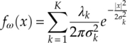
where 0 < α ≤ 2 is the characteristic exponent, δ is the total number of Gaussian components, λk is the probability of the noise ω being chosen from the kth component, and ![]() is the variance of the kth component.
is the variance of the kth component.
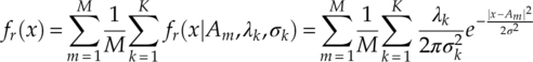
As the GMM will be used as the primary model for impulsive noise, therefore we derive the PDFs of received signals in the non-Gaussian channel with a GMM noise model. Assume the GMM uses K components where the probability λk and variance ![]() for each component are either known or estimated. The PDF of the complex signal in the non-Gaussian channel can be derived as equation (2.29),
for each component are either known or estimated. The PDF of the complex signal in the non-Gaussian channel can be derived as equation (2.29),
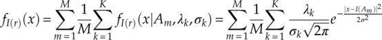
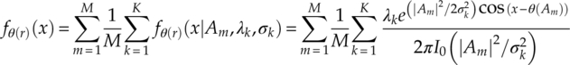
with the corresponding variation for signal I-Q segments, signal phase and signal magnitude given in equations (2.30), (2.31) and (2.32), respectively.

2.5 Conclusion
In this chapter, we establish the signal models required for constructing modulation classifiers in the following chapters. The signal models are also needed in the computer-aided simulations for the generation of signals for classification.
Three common communication channels, namely AWGN channel, fading channel, and non-Gaussian channel, are considered. The PDFs of received signals in the AWGN channel are derived for the complex signal, in-phase and quadrature segments, signal phase and signal magnitude in equations (2.5), (2.6), (2.7) and (2.12). The approximation of the PDF of signal phase in equation (2.7) is introduced into equation (2.9) as an alternative for easier theoretical analysis. An example of the approximate for M-PSK modulations is given in equation (2.10).
The fading channel has been divided into two scenarios of slow fading channel and fast fading channel. In the slow fading channel the PDF of received signal-experienced constant attenuation and phase offset are given in equation (2.14), while its variation for signal I-Q segments, signal phase and signal magnitude are listed in equations (2.15), (2.16) and (2.17). The signal model in fast fading channel is defined in equation (2.21) with attenuation and phase offset as normally distributed random processes. The additional signal model with frequency offset is given in equation (2.22).
Three non-Gaussian models are presented for modelling the impulsive noise. The PDF of Middleton’s Class A noise is given in equation (2.24), while the characteristic function of the alpha stable noise is given in equation (2.26). The Gaussian mixture model is suggested to approximate the Middleton’s Class A model and the alpha stable model. Its manageable PDF in equation (2.27) makes the derivation of the complex signal, signal I-Q segments, signal phase and signal magnitude distribution PDFs in equations (2.28), (2.29), (2.30) and (2.31) much more intuitive and any further analysis relatively effortless.
References
- Azzouz, E.E. and Nandi, A.K. (1996) Automatic Modulation Recognition of Communication Signals, Kluwer, Boston.
- Bennett, W.R. (1956) Methods of solving noise problems. Proceedings of the IRE, 44, 609–638.
- Chavali, V.G. and Da Silva, C.R.C.M. (2011) Maximum-likelihood classification of digital amplitude-phase modulated signals in flat fading non-Gaussian channels. IEEE Transactions on Communications, 59 (8), 2051–2056.
- Chavali, V.G. and Da Silva, C.R.C.M. (2013) Classification of digital amplitude-phase modulated signals in time-correlated non-Gaussian channels. IEEE Transactions on Communications, 61 (6), 2408–2419.
- Gallager, R.G. (2008) Principles of Digital Communication, Cambridge University Press, Cambridge.
- Goldsmith, A. (2005) Wireless Communications, Cambridge University Press, Cambridge.
- Huang, C.Y. and Polydoros, A. (1995) Likelihood methods for MPSK modulation classification. IEEE Transactions on Communications, 43 (2), 1493–1504.
- Middleton, D. (1999) Non-Gaussian noise models in signal processing for telecommunications: new methods and results for class A and class B noise models. IEEE Transactions on Information Theory, 45 (4), 1129–1149.
- Nikias, C.L. and Shao, M. (1995) Signal Processing with Alpha-Stable Distributions and Applications, John Wiley & Sons, Inc., New York.
- Shi, Q. and Karasawa, Y. (2012) Automatic modulation identification based on the probability density function of signal phase. IEEE Transactions on Communications, 60 (4), 1–5.
- Spooner, C.M. (1996) Classification of Co-channel Communication Signals Using Cyclic Cumulants. Conference Record of the Twenty-Ninth Asilomar Conference on Signals, Systems and Computers, Pacific Grove, CA, USA, 30 October 1995, pp. 531–536.
- Swami, A. and Sadler, B.M. (2000) Hierarchical digital modulation classification using cumulants. IEEE Transactions on Communications, 48 (3), 416–429.
- Urriza, P., Rebeiz, E., Pawełczak, P. and Čabrić, D. (2011) Computationally efficient modulation level classification based on probability distribution distance functions. IEEE Communications Letters, 15 (5), 476–478.
- Vastola, K.S. (1984) Threshold detection in narrow-band non-Gaussian noise. IEEE Transactions on Communications, C (2), 134–139.
- Wang, F. and Wang, X. (2010) Fast and robust modulation classification via Kolmogorov-Smirnov test. IEEE Transactions on Communications, 58 (8), 2324–2332.
- Wei, W. and Mendel, J.M. (2000) Maximum-likelihood classification for digital amplitude-phase modulations. IEEE Transactions on Communications, 48 (2), 189–193.
- Zhu, Z., Aslam, M.W. and Nandi, A.K. (2014) Genetic algorithm optimized distribution sampling test for M-QAMmodulation classification. Signal Processing, 94, 264–277.