
5
Modulation Classification Features
5.1 Introduction
In Chapters 3 and 4, two decision theoretic-based approaches to AMC are presented. For certain modulations such as AM and FM, it is obvious that signal distribution is not the only way to differentiate the two modulations. By analyzing the nature of the modulation technique, one can easily identify the key features of a signal modulated using a specific modulation scheme. While decision theoretic-based classifiers provide excellent classification accuracy, their high computational complexity motivates the development of feature-based classifiers which yield sub-optimal performance for much lower computational requirements.
In this chapter we list some of the well-recognized features designed for modulation classification. While the book focuses on digital modulations, features historically used for the classification of analogue modulations will also be included in this chapter. In the remainder of the chapter we first investigate the spectral-based features which exploits the spectral properties of different signal components. The wavelet-based features are given as another approach to feature-based modulation classification using the signal waveform. The high-order statistic features are examined as optioned to classifier digital modulations of different type and orders. The cyclic features based on cyclostationary analysis are presented at the end. More advanced feature-based (FB) classifiers which could utilize the features listed in this chapter are presented in Chapter 6.
5.2 Signal Spectral-based Features
Nandi and Azzouz proposed some key signal spectral-based features in the 1990s for the classification of basic analogue and digital modulations (Azzouz and Nandi, 1995, 1996b; Nandi and Azzouz, 1995). These key features generalized and advanced the works of Fabrizi, Lopes and Lockhart (1986), Chan and Gadbois (1989), and Jovanovic, Doroslovacki and Dragosevic (1990), which suggested different feature-extraction methods. The features exploit the unique spectral characters of different signal modulations in three key signal aspects, namely the amplitude, phase and frequency. Since different signal modulations exhibit different properties in their amplitude, phase and frequency, a complete pool of modulation candidates is broken down to sets and subsets which can be discriminated with the most effective features. A decision tree, consisting of nodes of sequential tests dedicated by different features, is often employed to give a clear guideline for the classification procedure.
In the following subsection, we first list these key features. Second, the features are analyzed for their capability in distinguishing different modulation sets. The section is concluded with some proposed classification decision trees suggested by Nandi and Azzouz for the classification of analogue and digital modulation.
5.2.1 Signal Spectral-based Features
The first feature, γmax, is the maximum value of the spectral power density of the normalized and centred instantaneous amplitude of the received signal (Azzouz and Nandi, 1996a), equation (5.1),
where DFT(-) is the discrete Fourier transform (DFT), Acn is the normalized and centred instantaneous amplitude of the received signal r, and N is the total number signal samples. The normalization is achieved by adopting equation (5.2),
where μA is the mean of the instantaneous amplitude of one signal segment, equation (5.3).
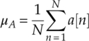
The normalization of the signal amplitude is designed to compensate the unknown channel attenuation.
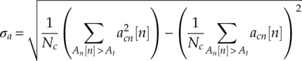
The second feature, σap, is the standard deviation of the absolute value of the non-linear component of the instantaneous phase, equation (5.4).
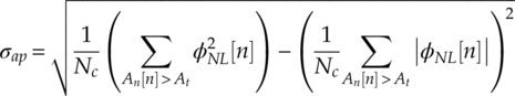
where Nc is the number of samples that meet the condition:An[n] > At. The variable At is a threshold value which filters out the low-amplitude signal samples because of their high sensitivity to noise. Term φNL[n] denotes the non-linear component of the instantaneous phase of the nth signal sample.
The third feature, σdp, is the standard deviation of the non-linear component of the direct instantaneous phase, given by equation (5.5),
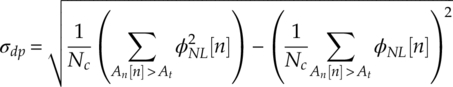
where all parameters remain the same as in the expression for σap. However, it is noticeable that the absolute operation on the non-linear component of the instantaneous phase is removed.
The fourth feature, P, is an evaluation of the spectrum symmetry around the carrier frequency, evaluated by equation (5.6),
where equations (5.7) and (5.8) hold, such that when
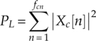
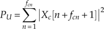
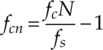
Xc[n] is the Fourier transform of the signal xc[n], (fcn + 1) is the sample number corresponding to the carrier frequency fc, and fs is the sampling rate, the equation (5.9) holds.
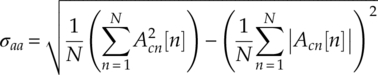
The fifth feature, σaa, is the standard deviation of the absolute value of the normalized and centred instantaneous amplitude of the signal samples, given by equation (5.10).
The sixth feature, σaf, is the standard deviation of the absolute value of the normalized and centred instantaneous frequency, given by equation (5.11),
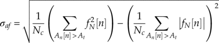
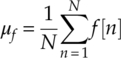
where the centred instantaneous frequency fm is normalized by the sampling frequency fs such that equation (5.12) applies.
The instantaneous frequency is centred using the frequency mean μf as shown in equations (5.13) and (5.14).
The seventh feature, σa, is the standard deviation of the normalized and centred instantaneous amplitude [equation (5.15)].
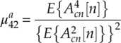
The eighth feature, ![]() , is the kurtosis of the normalized and centred instantaneous amplitude, given by equation (5.16).
, is the kurtosis of the normalized and centred instantaneous amplitude, given by equation (5.16).
The ninth feature, ![]() , is the kurtosis of the normalized and centred instantaneous amplitude [equation (5.17)].
, is the kurtosis of the normalized and centred instantaneous amplitude [equation (5.17)].

5.2.2 Spectral-based Features Specialities
Having defined all of Nandi and Azzouz’s signal spectral-based features, next we will analyze every key feature and suggest their usage in modulation classification. Building on Nandi and Azzouz’s work, we have added PAM and QAM modulation to enrich the analysis of the features in a more up-to-date context.
The quantity γmax measures the variance in signal instantaneous amplitude. For modulations, where information is conveyed in the signal amplitude, the value of γmax should be non-zero. One the other hand, for modulations with constant amplitude, the value of γmax should be zero. Thus, we have two sets of modulations which can be classified by γmax and a corresponding threshold ![]() . The first set of modulations includes AM single-sideband modulation (SSB), M-ASK, M-PAM, M-PSK and M-QAM. The second set of modulations includes FM and M-FSK.
. The first set of modulations includes AM single-sideband modulation (SSB), M-ASK, M-PAM, M-PSK and M-QAM. The second set of modulations includes FM and M-FSK.
Quantity σap measures the variance in the absolute instantaneous phase. The first set of modulations includes FM, SSB, M-FSK, M-PSK (M ≥ 2), M-QAM. The second set of modulations includes AM, M-ASK, BPSK. BPSK does not have information in its absolute instantaneous phase (centred), because there are only two states for the instantaneous phase. When the instantaneous phase is centred at zero, their absolute values are the same.
Quantity σdp measures the variance in the absolute instantaneous phase. The first set of modulations includes FM, SSB, M-FSK, M-PSK, M-QAM. The second set of modulations includes AM, M-ASK. Being similar to σap, σdp provides the ability to distinguish BPSK from other modulations without phase information.
Quantity P provides the criterion to classify different amplitude-based modulations with different properties in the frequency domain. One set of the modulations has a symmetrical spectrum arrangement about the carrier frequency. They include AM and double-sideband modulation (DSB). The other, obviously with asymmetrical spectrum density about the carrier frequency, includes vestigial sideband (VSB), lower sideband modulation (LSB) and upper sideband modulation (USB).
Quantity σaa measures the amount of information in the signal’s instantaneous amplitude. This feature is similar to γmax. However, it is gifted with the extra ability to differentiate 2-ASK from other M-ASK modulations. This is because the absolute values of 2-ASK signal’s instantaneous amplitude become identical when they are centred at zero.
Quantity σaf is primarily designed for the classification of 2-FSK and 4-FSK modulations. The theoory that it can enable discrimination is same as that for σap and σaa, where the frequency information of the binary-state modulation is removed by taking the absolute value of the centred instantaneous frequency.
Quantity ![]() measures the compactness of the instantaneous amplitude distribution. AM modulation, being an analogue modulation with varying instantaneous amplitude, has a less compact distribution compared with digital modulations such as M-ASK modulations.
measures the compactness of the instantaneous amplitude distribution. AM modulation, being an analogue modulation with varying instantaneous amplitude, has a less compact distribution compared with digital modulations such as M-ASK modulations.
Quantity ![]() measures the compactness of the instantaneous frequency distribution. Like AM modulation, FM has less compact frequency distribution compared with digital modulations such as M-FSK, because of its analogue instantaneous frequency.
measures the compactness of the instantaneous frequency distribution. Like AM modulation, FM has less compact frequency distribution compared with digital modulations such as M-FSK, because of its analogue instantaneous frequency.
5.2.3 Spectral-based Features Decision Making
Azzouz and Nandi (1995, 1996a, 1996b) designed decision trees for the classification of analogue and digital modulations. The trees consist of an input node where all the features are extracted and imported. The input node is followed by a sequence of conditional or decision steps facilitated with selected individual features. In this section, we have reorganized these decision trees and created a decision tree in Figure 5.1 for the classification of the aforementioned modulations.
Figure 5.1 Decision tree for modulations classification using spectral-based features.
The diamond block in Figure 5.1 represents a conditional sub-stage classification, with t(-) being the suitable threshold for different features.
5.2.4 Decision Threshold Optimization
To establish the decision threshold for each spectral-based feature, pilot samples could be used to achieve that. Assume we have L signal realizations from group A and L signal realizations from group B, where the two groups of modulations can be classified using feature ![]() . The optimal threshold can be calculated as shown in equation (5.18),
. The optimal threshold can be calculated as shown in equation (5.18),
where ![]() and
and ![]() are the standard deviations of the feature values calculated using signals from group A and group B, respectively, using equations (5.19) and (5.20),
are the standard deviations of the feature values calculated using signals from group A and group B, respectively, using equations (5.19) and (5.20),
and ![]() and
and ![]() are the means of the features values from each group, equations (5.21) and (5.22).
are the means of the features values from each group, equations (5.21) and (5.22).
5.3 Wavelet Transform-based Features
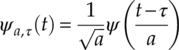
The continuous wavelet transform of received signal r is defined as the integral of r(t) times the conjugate transpose of the wavelet function ψa,τ(t) over time, equation (5.23).
Among different mother wavelet functions, namely Morlet, Haar and Shannon, most researchers selected the Haar wavelet function because of its simple form and computational convenience. The Haar wavelet is given by equation (5.24),
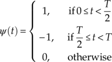
which can be scaled and translated to create a series of baby wavelets [equation (5.25)].
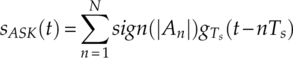
To enable the analysis of the continuous wavelet transform (CWT) for different modulation signals, we first established individual expressions of the transmitted signal from each modulation. For M-ASK the representation of its transmitted signal is given by equation (5.26),
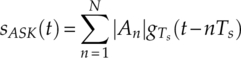
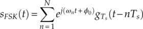
where |An|∈ {|A1|, |A2| … |AM|} is the nth symbol being transmitted, with M being the total number of states, and ![]() is the pulse-shaping function of duration Ts. The expression for the M-FSK is given by equation (5.27),
is the pulse-shaping function of duration Ts. The expression for the M-FSK is given by equation (5.27),
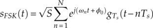
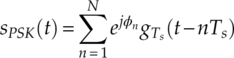
where S is average signal power, ωn ∈ {ω1, ω2 … ωM} is the signal frequency at the nth symbol, and φ0 is the initial carrier phase. For PSK, the expression is given by equation (5.28),
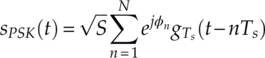
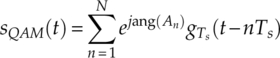
where φn ∈ {φ1, φ2 … φM} is the phase of the nth symbol. Lastly, the expression for the QAM modulation signal is defined by equation (5.29),
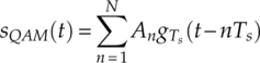
where An ∈ {A1, A2 … AM} is the complex envelope of the nth symbol being transmitted.
The derivation for ASK modulations in a noise-free environment is produced by Hassan et al. (2010) in the form of equation (5.30).
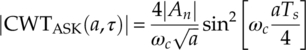
The corresponding CWT for FSK, PSK and QAM is derived by Hong and Ho (2000), as equations (5.31)–(5.33), respectively.
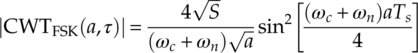
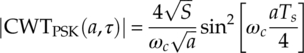
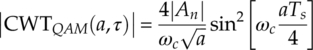
It is obvious that the CWT of PSK is a constant, while others modulations all have multi-step functions as their CWT. Thus PSK can be distinguished from other modulations using the CWT. To classify FSK modulation, we examine the CWT of these modulations when they are normalized by amplitude [equation (5.34)].

The updated expressions for the transmitted symbols are given below in equations (5.35)–(5.38).
It is not difficult to see that, for normalized signals, the variance in CWT is only seen for FSK modulations. Therefore, the CWT for normalized signals can be used as a feature for the classification of FSK modulations. Having achieved the classification of PSK and FSK, the only task left is to differentiate between ASK and QAM modulations. As there is no obvious distinction between the CWTs of these two modulation types, Hassan et al. (2010) suggested using the high-order moments and cumulants to exploit the small differences between these two modulation types. In addition, the application of the high-order moments and cumulants also enables the intra-class classification when modulation of a different order is involved. Because there is a separate section dedicated to high-order statistical features in this chapter, the high-order moments and cumulants will be presented in the corresponding section.
5.4 High-order Statistics-based Features
In this section, we focus on the high-order statistics (HoS)-based features, more specifically moment-based and cumulant-based features.
5.4.1 High-order Moment-based Features
Hipp was the first to adopt the third-order moment of the demodulated signal amplitude as a modulation-classification feature (Hipp, 1986). Since we consider the demodulated signal as a luxury for any modulation classifier, this moment-based feature is not investigated in this book.
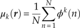
The usage of moments in modulation classification was later extended by Soliman and Hsue, who investigated the high-order moments of the signal phase for the classification of M-PSK modulations (Soliman and Hsue, 1992). They derived the theoretical kth moment of signal phase in Gaussian channel which leads to the conclusion that the moments are a monotonically increasing function with respect to the order of the M-PSK modulation. Thus, high-order M-PSK modulations have higher moment values, which provide the condition for the classification of M-PSK modulations of different orders. Meanwhile, Soliman and Hsue also made the observation that the difference in moment value between higher-order modulations is not distinct for lower-order moments. Therefore, they concluded that the effective classification of M-PSK modulation with higher order requires the moments of higher order. The calculation of the kth order moment of the signal phase is defined as shown in equation (5.39),
where φ(n) is the phase of the nth signal sample. Azzouz and Nandi (1996a) proposed the kurtosis of the normalized-centred instantaneous amplitude ![]() and the kurtosis of the normalized-centred instantaneous frequency
and the kurtosis of the normalized-centred instantaneous frequency ![]() for the classification of M-ASK and M-FSK modulations. The expressions for these two features are given in equations (5.16) and (5.17). Hero and Hadinejad-Mahram generalized the moment-based features to include the high-order moment of signal phase and frequency magnitude (Hero and Hadinejad-Mahram, 1998). Spooner employed high-order cyclic moments as features (along with cyclic moments) for the classification of modulation with identical cyclic autocorrelation functions (Spooner, 1996).
for the classification of M-ASK and M-FSK modulations. The expressions for these two features are given in equations (5.16) and (5.17). Hero and Hadinejad-Mahram generalized the moment-based features to include the high-order moment of signal phase and frequency magnitude (Hero and Hadinejad-Mahram, 1998). Spooner employed high-order cyclic moments as features (along with cyclic moments) for the classification of modulation with identical cyclic autocorrelation functions (Spooner, 1996).
In this book we use the following expression to calculated different kth moment of the complex-valued signal r = r[1], r[2], …, r[N] [equation (5.40)],
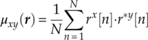
where x + y = k and r*[n] is the complex conjugate of r[n].
5.4.2 High-order Cumulant-based Features
Swami and Sadler (2000) suggested the fourth-order cumulant of the complex-valued signal as features for the classification of M-PAM, M-PSK and M-QAM modulations. For signal r[n] the second-order moments can be defined in either of two different ways [equations (5.41) and (5.42)].
Likewise, the fourth-order moments and cumulants can be expressed in three different ways using different placements of conjugation [equations (5.43)–(5.45)],
where cum(·) is joint cumulant function defined by equation (5.46).
Meanwhile, the estimation of the second and fourth cumulants is achieved by using the following processes as shown in equations (5.47)–(5.51).
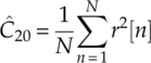
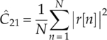
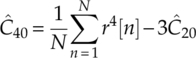
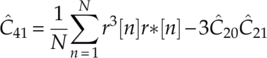
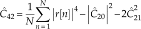
Table 5.1 Decision tree for modulations classification using spectral-based features
| C20 | C21 | C40 | C41 | C42 | |
| 2-PAM | 1.0000 | 1.0000 | −2.0000 | −2.0000 | −2.0000 |
| 4-PAM | 1.0000 | 1.0000 | −1.3600 | −1.3600 | −1.3600 |
| 8-PAM | 1.0000 | 1.0000 | −1.2381 | −1.2381 | −1.2381 |
| BPSK | 1.0000 | 1.0000 | −2.0000 | −2.0000 | −2.0000 |
| QPSK | 0.0000 | 1.0000 | 1.0000 | 0.0000 | −1.0000 |
| 8-PSK | 0.0000 | 1.0000 | 0.0000 | 0.0000 | −1.0000 |
| 4-QAM | 0.0000 | 1.0000 | 1.0000 | 0.0000 | −1.0000 |
| 16-QAM | 0.0000 | 1.0000 | −0.6800 | 0.0000 | −0.6800 |
| 64-QAM | 0.0000 | 1.0000 | −0.6191 | 0.0000 | −0.6191 |
Cumulant values for some noise-free modulation signals are listed in Table 5.1. It is clear from Table 5.1 that different modulations have different cumulant values between each other. Thus the classification of these modulations can be realized. The classification decision making could be achieved with a decision where modulations are divided into subgroups for each cumulant. The decision threshold can be defined using the process suggested in Section 5.2.4.
5.5 Cyclostationary Analysis-based Features
Gardner pioneered the area of signal cyclostationary analysis, which exploits the periodic properties of a cyclostationary process (Gardner, 1994). Gardner and Spooner first implemented cyclostationary analysis for modulation classification problems (Gardner and Spooner, 1988), exploiting the distinct differences between the cyclic spectrum patterns of different modulations. The implementation is well summarized in Ramkumar’s tutorial on cyclic features detection (Ramkumar, 2009).
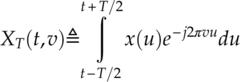
Give a sinusoidal signal x(t), it exhibits cyclostationary properties or contains second-order periodicity if the cyclic autocorrelation shown in equation (5.52) exists with
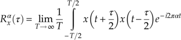
frequency α ≠ 0 and is not identically zero as a function of τ. The Fourier transform of the cyclic autocorrelation is given by equation (5.53),
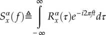
known as the cyclic spectrum. The cyclic spectrum can be interpreted as a spectral correlation function (SCF) as defined in equation (5.54),
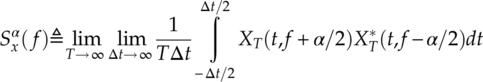
where equation (5.55) holds.
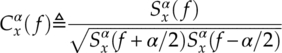
Gardner demonstrated that the theoretical SCF plane of different modulation signals over a domain of α and f has distinctive differences and can be used for the classification of signal modulations (Gardner, 1994). The correlation coefficient, known as spectral coherence (SC), of the SCF is defined as shown in equation (5.56).
To reduce the dimension of the cyclic spectrum, it is possible to construct a cyclic domain profile (CDP) by finding the maximum of SC over frequency f [equation (5.57)] (Kim et al., 2007).
The CDP preserves the distinction of cyclic properties between different modulation signals. It can be used for modulation classification.
While the SCF and CDP can be used for the classification of some lower-order modulations, they are not suitable for higher-order modulations. For this reason, Spooner proposed the use of cyclic cumulants for the classification of high-order modulations (Spooner, 1996). The cyclic cumulants of higher order were suggested by Dobre, Bar-Ness and Su (2003).
The nth moments of x(t) are defined as shown in equation (5.58),
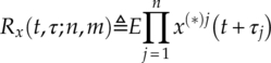
where n is the order,τ = [τ1 … τn] is the delay vector, (*)j is an optional conjugate, and m is the number of conjugate factors. The nth-order cumulants are defined as shown in equation (5.59),
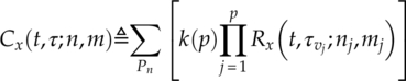
where Pn is the set of partitions of {1,2,…,n}, nj is the size of the set vj, mj is the number of conjugated terms in the term ![]() , and k(p) is the number (−1)
p − 1(p − 1) !. The cumulant function is also representable by a generalized Fourier series as given in equation (5.60),
, and k(p) is the number (−1)
p − 1(p − 1) !. The cumulant function is also representable by a generalized Fourier series as given in equation (5.60),
where β is called a pure nth-order cycle frequency, and ![]() is the nth-order temporal cumulant function or cyclic cumulant.
is the nth-order temporal cumulant function or cyclic cumulant.
For digital modulations such as QAM modulations, the cyclic cumulants can be defined as shown in equation (5.61),
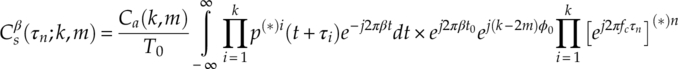
where Ca(k, m) is the kth-order cumulant with m conjugates. The final feature used for modulation classification is the maximum value of the function ![]() , given a set of different n, m, and β [equation (5.62)].
, given a set of different n, m, and β [equation (5.62)].
5.6 Conclusion
In this chapter, we list a collection of signal features that can be used for modulation classifiers. The spectral features are well established and suitable for the classification of both analogue and digital modulations. The high-order statistics features including moments, cumulants and cyclic cumulants focus on the classifier of high-order digital modulations. The actual classification process of a feature-based classifier requires the construction of a decision tree where the modulations must be divided into several tiers of subgroups until each modulation could be differentiated from the rest. The easiest decision-making process for a feature-based classifier requires the threshold to be set at each decision-making point on the decision tree. The threshold could be calculated using a theoretical noise-free signal or optimized with given channel conditions.
References
- Azzouz, E.E. and Nandi, A.K. (1995) Automatic identification of digital modulation types. Signal Processing, 47 (1), 55–69.
- Azzouz, E.E. and Nandi, A.K. (1996a) Automatic Modulation Recognition of Communication Signals, Kluwer, Boston.
- Azzouz, E.E. and Nandi, A.K. (1996b) Procedure for automatic recognition of analogue and digital modulations. IEE Proceedings – Communications, 143 (5), 259–266.
- Chan, Y.T. and Gadbois, L.G. (1989) Identification of the modulation type of a signal. Signal Processing, 1 (4), 838–841.
- Dobre, O.A., Bar-Ness, Y. and Su, W. (2003) Higher-Order Cyclic Cumulants for High Order Modulation Classification. Military Communications Conference, 13–16 October 2003, IEEE, pp. 112–117.
- Fabrizi, P.M., Lopes, L.B. and Lockhart, G.B. (1986) Receiver Recognition of Analogue Modulation Types. Proceedings of the IERE Conference on Radio Receiver and Associated Systems, IERE, pp. 135–140.
- Gardner, W.A. (1994) Cyclostationarity in Communications and Signal Processing, IEEE Press, New York.
- Gardner, W.A. and Spooner, C.M. (1988) Cyclic spectral analysis for signal detection and modulation recognition. Military Communications Conference, 1988, MILCOM, pp. 419–424. Conference record. 21st Century Military Communications - What's Possible? 1988 IEEE, vol. 2, pp. 419, 424, 23–26 Oct. 1988. doi: 10.1109/MILCOM.1988.13425
- Hassan, K., Dayoub, I., Hamouda, W. and Berbineau, M. (2010) Automatic modulation recognition using wavelet transform and neural networks in wireless systems. EURASIP Journal on Advances in Signal Processing, 2010, 1–13.
- Hero, A.O. and Hadinejad-Mahram, H. (1998) Digital modulation classification using power moment matrices. Proceedings of the 1998 IEEE International Conference on Acoustics, Speech, and Signal Processing, 12–15 May 1998, vol. 6, pp. 3285–3288.
- Hipp, J.E. (1986) Modulation Classification Based on Statistical Moments. Military Communications Conference, - Communications-Computers: Teamed for the 90’s, 1986. MILCOM 1986, 5–9 October 1986, IEEE, vol. 2, pp. 20.2.1–20.2.6 doi: 10.1109/MILCOM.1986.4805739.
- Hong, L. and Ho, K.C. (2000) BPSK and QPSK Modulation classification with unknown signal level. Military Communications Conference Proceedings, vol. 2, pp. 976–980. doi: 10.1109/MILCOM.2000.904076.
- Jovanovic, S.D., Doroslovacki, M.I. and Dragosevic, M.V. (1990) Recognition of Low Modulation Index AM Signals in Additive Gaussian Noise. Proceedings of the European Association for Signal Processing V Conference, EURASIP, pp. 1923–1926.
- Kim, K., Akbar, I.A., Bae, K.K. et al. (2007) Cyclostationary Approaches to Signal Detection and Classification in Cognitive Radio. IEEE International Symposium on New Frontiers in Dynamic Spectrum Access Networks, pp. 212–215.
- Nandi, A.K. and Azzouz, E.E. (1995) Automatic analogue modulation recognition. Signal Processing, 46, 211–222.
- Ramkumar, B. (2009) Automatic modulation classification for cognitive radios using cyclic feature detection. IEEE Circuits and System Magazine, 9 (2), 27–45.
- Soliman, S.S. and Hsue, S.-Z. (1992) Signal classification using statistical moments. IEEE Transactions on Communications, 40 (5), 908–916.
- Spooner, C.M. (1996) Classification of co-channel communication signals using cyclic cumulants. 1995 Conference Record of the Twenty-Ninth Asilomar Conference on Signals, Systems and Computers, 30 October–1 November 1995, vol. 1, pp. 531–536. doi: 10.1109/ACSSC.1995.540605.
- Swami, A. and Sadler, B. M. (2000) Hierarchical Digital Modulation Classification Using Cumulants. IEEE Transactions on Communications, 48 (3), 416–429.