
7
Blind Modulation Classification
7.1 Introduction
From Chapters 3–6, we listed modulation classifiers of different types. These classifiers mostly require the prior knowledge of channel state information (Wei and Mendel, 2000; Wang and Wang, 2010). There are few classifiers which have the certain ability to treat one or two channel parameters as unknown (Panagiotou, Anastasopoulos and Polydoros, 2000). Many classifiers may appear to be able to recognize the modulation type without the need for CSI (Azzouz and Nandi, 1996; Spooner, 1996; Swami and Sadler, 2000). In fact, the classification accuracy is often far inferior if the CSI is not utilized for the preparation of reference values or decision thresholds. Dobre et al. reviewed some of the semi-blind classifiers and suggested the necessity of a blind modulation classifier (Dobre, Abdi and Bar-Ness, 2005).
The classification of modulation types in a channel with unknown CSI is normally divided into two steps. In the first step, channel estimation is performed. The estimation can either acquire all of the needed channel parameters or partial CSI. When the entire CSI is estimated, any classifier that we have mentioned in the previous chapters can be employed to complete the second step. If the CSI is partially estimated, a classifier which requires the prior knowledge of all channel parameters will not be able to complete the classification. Instead, a semi-blind classification that can complement the partial channel estimation is required to complete the second step of the blind modulation classification (BMC).
In this chapter, we present a few recently published blind modulation classification approaches which operate with unknown CSI. The first relies on maximum likelihood estimation realized in an unsupervised way through expectation maximization. The modulation classification is completed using a likelihood-based classifier which utilizes the estimated CSI. The second is a combination of minimum distance centroid estimation and likelihood-based classifier using non-parametric likelihood function.
7.2 Expectation Maximization with Likelihood-based Classifier
As stated in Chapter 3, to achieve optimal classification performance, the likelihood-based classifiers such as the ML classifier require perfect knowledge of the CSI. In normal systems where modulations are known to the receiver, the estimation is relatively easy, especially with pilot samples. In the system with AMC, the modulation is unknown to the receiver and thus cannot be used in the estimator. While an estimator for signals with unknown modulation is available (Gao and Tepedelenlioglu, 2005), the estimation accuracy is not high enough to guarantee high classification accuracy. In addition, such estimators are normally limited to modulations of the same type but different orders. When there are more than two types of modulation in the candidate pool such estimators are not applicable for the CSI estimation for likelihood-based classifiers. It is worth noting that the ALRT, GLRT, and HLRT classifiers could be constructed to achieve maximum likelihood estimation of a channel parameter. The estimation is achieved through an exhaustive manner which requires the evaluation of likelihood for each value of channel parameter in a predefined range, which is highly expensive computationally. The matter is made worse when multiple channel parameters need to be estimated jointly. For this reason, iterative processes such as expectation maximization (EM) (Geoffrey and Peel, 2000) have become a more realistic option for channel estimation (Moon, 1996; Tzikas, Likas and Galatsanos, 2008).
7.2.1 Expectation Maximization Estimator
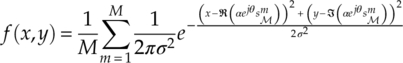
For modulation classification, Chavali and Da Silva first proposed to use EM for CSI estimation (Chavali and Da Silva, 2011) and considered the case of non-Gaussian noises (Chavali and Da Silva, 2013). Here, we present the algorithm in a more recognizable AWGN channel. In EM, we assume there are a set of channel parameters Θ = {γm, μm, σm}. A Gaussian mixture model is often considered as an integral part of an EM estimator for modulation classification. A GMM is a linear mixture of Gaussian distributed components. The PDF of a GMM model is given by equation (7.1),
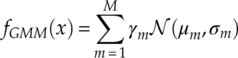
where γm is the mixture proportion of the mth component, and μm and σm are the corresponding mean and variance.
The initial step of EM is to provide initial values for the channel parameters. There are two most popular ways to do this. The first method generates random values for the channel parameters Θ = {γm, μm, σm}. It is easy to implement and adds a minimum amount of extra computation. The disadvantage of this random initialization method is that the time for convergence may be longer and the converged final estimate may be a local optimum instead of a global optimal estimate. The other, more advanced, approach to initialization is to use a fast algorithm to provide a rough estimation for some of the parameters. Soltanmohammadi and Naraghi-Pour used K-means clustering for the initialization step (Soltanmohammadi and Naraghi-Pour, 2013). By clustering all the samples into M number of partitions, the proportion of the Gaussian component can be calculated using the size of the partition, that is, the number of samples assigned to the partition. The mean of the component can be calculated using the mean of all the signal samples in each partition. The variance of each component can be calculated in the same way using the partitioned signal samples.
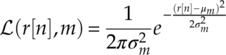
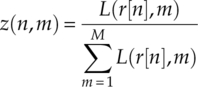
The expectation step, also known as the E step, evaluates the likelihood of each sampling belongs to each of the Gaussian components. A membership is often assigned using the resulting likelihood values. The membership could be a hard membership which assigns the signal sample to an individual Gaussian component exclusively. Meanwhile, the sample can be given soft memberships for all the Gaussian components, where components with higher likelihood are assigned higher membership values. The membership is often called a latent variable z. For the signal samples r[1], r[2] … r[N] the likelihood of the nth sampling belonging to the mth component of the GMM model is calculated as shown in equation (7.2).
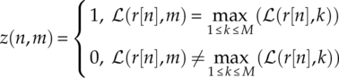
And the corresponding soft membership is calculated as shown in equation (7.3)
with the hard membership assigned as shown in equations (7.4).
The membership of each signal sample having been evaluated, the maximization step aims to maximize the evaluated log-likelihood function of the current iteration, equation (7.5).
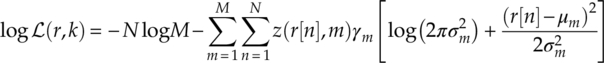
For modulation classification, there is underlying structure of the component means which can be expressed as a combination of channel gain and transmitted symbols, as given in equation (7.6),
where h is the channel coefficient and sm is the mth symbol in the modulation alphabet set. In the meantime, the noise variances of each Gaussian component are often considered identical [equation (7.7)].
The maximization step is achieved by the close form update function of the current likelihood evaluation. Combining equations (7.5)–(7.7), the derivative with respect to channel coefficient and noise variance can be calculated as shown in equations (7.8) and (7.9).
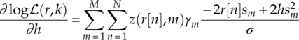
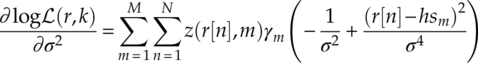
When equations (7.8) and (7.9) are set to zero, the update function for the channel gain and the variance are given by equations (7.10) and (7.11),

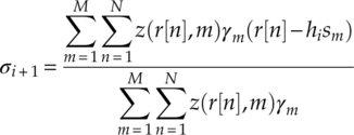
where hi + 1 and σi + 1 are the updated estimation of the parameters for iteration i + 1. In equation (7.11), the channel coefficient estimated in the previous iteration is used, which makes this the update function of the expectation/condition maximization (ECM) algorithm. It is often adopted to deal with coupling parameters such as the channel coefficient and the noise variance in this case. ECM shares the convergence property of EM (Meng and Rubin, 1993) and can be constructed to converge at a similar rate as the EM algorithm (Sexton, 2000).
The iterative process is terminated under two conditions. The first condition terminates the process when the estimation reaches convergence. The condition is represented numerically with the difference between the expected likelihoods of the current iteration and the previous iteration along with a pre-defined threshold. In the second condition, termination is triggered when the pre-defined number of iterations has been reached.
7.2.2 Maximum Likelihood Classifier
For modulation classification, given the modulation candidate pool ![]() , the EM estimation is performed for each modulation hypothesis
, the EM estimation is performed for each modulation hypothesis ![]()
![]() ;(i)(i = 1, 2, … I). As demonstrated in Figure 7.1, the channel parameter set
;(i)(i = 1, 2, … I). As demonstrated in Figure 7.1, the channel parameter set ![]() is estimated for each modulation hypothesis, with
is estimated for each modulation hypothesis, with ![]() being the EM estimated complex channel gain and
being the EM estimated complex channel gain and ![]() being the estimated signal variance for modulation candidate
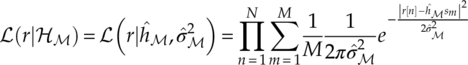
being the estimated signal variance for modulation candidate ![]() ;(i). Subsequently the likelihood for each modulation hypothesis is evaluated using the corresponding channel estimation. Here we use the likelihood function from equation (3.3); however, we replace the known channel parameters with EM estimates, to arrive at equation (7.12).
;(i). Subsequently the likelihood for each modulation hypothesis is evaluated using the corresponding channel estimation. Here we use the likelihood function from equation (3.3); however, we replace the known channel parameters with EM estimates, to arrive at equation (7.12).
Figure 7.1 EM estimation and ML classifier.
It is worth noting that the complex channel gain consists of carrier phase offset estimation. When it is applied to the transmitted symbol sm the effect of constant phase offset is effectively compensated. The resulting likelihood values from all modulation hypotheses are then compared in order to conclude the classification decision. Using the maximum likelihood criteria equation (3.13), the modulation hypothesis with the highest likelihood is assigned as the classification decision.
7.2.3 Minimum Likelihood Distance Classifier
While the combination of EM estimation and ML classifier seems a perfect match, the combination has some fundamental flaws. The flaw is, in fact, shared with any method that combines a maximum likelihood estimator and a maximum likelihood classifier. As the channel estimation is performed under each modulation hypothesis, the channel estimation maximizes the likelihood evaluation of the modulation hypothesis regardless of whether the hypothesis is true or false. Compared with an ML classifier with given channel knowledge, the likelihood evaluation for the true hypothesis may be accurately achieved. However, because of the ML estimation the likelihood evaluation for false hypothesis is certainly increased, which leads to a reduced separation between the likelihood of the true hypothesis and the false hypotheses. In extreme cases it is even possible for the false modulation hypothesis to provide a higher likelihood value as compared with the true modulation hypothesis.
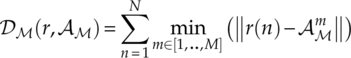
The above phenomenon is discussed by Soltanmohammadi and Naraghi-Pour, who also suggested a minimum distance likelihood classifier to overcome the issue (Soltanmohammadi and Naraghi-Pour, 2013). Instead of comparing the likelihood value from each modulation hypothesis directly, the distance between the observed likelihood is compared with the empirical likelihood of each modulation with the given channel estimation. The empirical likelihood values can be either computed beforehand and stored in memory or calculated using the channel estimation during the modulation classification processing. For the observed signal, there exist I likelihood values evaluated from different hypotheses denoted as {![]() (r|
(r|![]()
![]() ;(1), Θ
;(1), Θ![]() ;(1)),
;(1)), ![]() (r|
(r|![]()
![]() ;(2), Θ
;(2), Θ![]() ;(2)),…,
;(2)),…, ![]() (r|
(r|![]()
![]() ;(I), Θ
;(I), Θ![]() ;(I))}. Meanwhile, for each hypothesis
;(I))}. Meanwhile, for each hypothesis ![]()
![]() ;(i), there exists a set of empirical likelihood values denoted as {
;(i), there exists a set of empirical likelihood values denoted as {![]() ,
, ![]() ,…,
,…, ![]() }. The distance between the observed likelihood value set and empirical likelihood set from HM(i) is calculated as shown in equation (7.13).
}. The distance between the observed likelihood value set and empirical likelihood set from HM(i) is calculated as shown in equation (7.13).
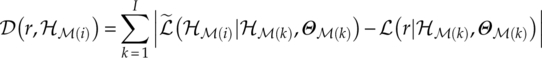
The subsequent classification decision is then acquired by finding the modulation hypothesis that provides the minimum likelihood distance, equation (7.14).
7.3 Minimum Distance Centroid Estimation and Non-parametric Likelihood Classifier
While EM estimation provides accurate joint estimation of the channel parameters, the estimation is still based on a known noise model. If unknown noise type with mismatching model is observed, the estimation accuracy is not guaranteed. In addition, being more efficient than an exhaustive estimator, the EM estimator is still relatively complex where multiple instances of likelihood evaluation are required to obtain the estimation. Seeking for alternative blind modulation classification solutions, Zhu and Nandi proposed a scheme to combine joint estimation of channel gain and phase offset with non-parametric likelihood function for BMC (Zhu and Nandi, 2014).
7.3.1 Minimum Distance Centroid Estimation
The minimum distance centroid estimator is an iterative process for the joint estimation of channel gain and phase offset. A signal-to-centroids distance metric is proposed to evaluate the mismatch between the estimation being updated and the observed signal. The method is based on the iterative update of a signal centroid collection composed of the original transmitted alphabet, the channel gain and phase shift. We assume the estimated centroids ![]() to possess the original rigid structure after transmission and pre-processing. The mean of centroids
to possess the original rigid structure after transmission and pre-processing. The mean of centroids ![]() should remain at 0, the magnitude of two different centroid elements
should remain at 0, the magnitude of two different centroid elements ![]() and
and ![]() should follow the original proportions
should follow the original proportions ![]() , and the phase difference between centroids should remain the same,
, and the phase difference between centroids should remain the same, ![]() . For BPSK, QPSK and 8-PSK the centroid collection is given by equations (7.15)–(7.17), respectively,
. For BPSK, QPSK and 8-PSK the centroid collection is given by equations (7.15)–(7.17), respectively,
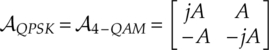
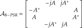
where A is defined as the centroid parameter, given by equation (7.18),
where ![]() is defined as the transmitted symbol which is nearest to the signal mean.
is defined as the transmitted symbol which is nearest to the signal mean.
The signal-to-centroid distance is defined as the sum of the Euclidean distance between each signal sample and its nearest centroid, as defined in equation (7.19).
It is worth noting that the above distance is an equivalent to the evaluation function of minimum distance classifier presented in Chapter 3 (Wong and Nandi, 2008).
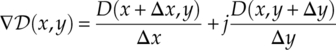
With the complex representation of the centroid parameter, A = x + jy, the signal-to-centroid distance can be expressed with x and y. To find the values of x and y which minimize the signal-to-centroid distance, we use an iterative sub-gradient method based on the sub-gradient calculation shown in equation (7.20).
Meanwhile, the update function for An = xn + jyn is expressed as given in equation (7.21),
where a is the update step size. A smaller update step size slows down convergence but provides a more accurate estimation. A bigger update step size helps the estimator converge faster but with the risk of lower estimation accuracy.
The process is repeated for a number of iterations unless the exit condition is triggered by convergence with a given threshold, equation (7.22),
where ![]() is a pre-defined threshold.
is a pre-defined threshold.
Given the estimated centroid parameter ![]() , the effective estimation of the channel gain and phase offset can be calculated as shown in equations (7.23) and (7.24), respectively.
, the effective estimation of the channel gain and phase offset can be calculated as shown in equations (7.23) and (7.24), respectively.

It is worth noting that the effective estimation of the phase offset is not accuracy. The estimation itself could be offered by a factor of mΔθ, where Δθ is the phase difference between adjacent modulation symbols. However, the offset should not affect the modulation classification performance since the likelihood evaluation takes the average of the likelihood from all modulation symbols.
7.3.2 Non-parametric Likelihood Function
As demonstrated, the MD estimator is able to find the centroid after transmission; however, the estimation of noise variance is absent. For this reason, the state-of-the-art likelihood classifier is not applicable in this case. To overcome this issue, Zhu and Nandi proposed a non-parametric likelihood function for the evaluation of likelihood without noise variance (Zhu and Nandi, 2014). The NPLF has been suggested in Chapter 3 as an LB approach with reduced complexity. In addition, the NPLF does not impose a hypothesized noise model. The NPLF is defined as given in equation (7.25),
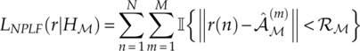
where ![]() {·} is an indicator function which returns 1 if the input is true and 0 if input is false, and the test radius
{·} is an indicator function which returns 1 if the input is true and 0 if input is false, and the test radius ![]()
![]() ; is given by equation (7.26),
; is given by equation (7.26),
with ![]() 0 being the reference radius. The non-parametric likelihood function is effectively the empirical estimation of the cumulative probability of the given signal in a set of defined local regions. The expectation of the likelihood can be expressed in the following manner [equation (7.27)],
0 being the reference radius. The non-parametric likelihood function is effectively the empirical estimation of the cumulative probability of the given signal in a set of defined local regions. The expectation of the likelihood can be expressed in the following manner [equation (7.27)],
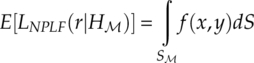
where S
![]() ; is a limit associated with both estimated centroids
; is a limit associated with both estimated centroids ![]() and the test radius
and the test radius ![]()
![]() ;, and f(x, y) is the probability density function of the testing signal.
;, and f(x, y) is the probability density function of the testing signal.
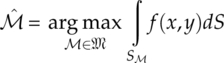
It is easy to see that, with the given testing radius, the area of ![]() is designed to give each hypothesis an equal area for the cumulative probability calculation. The decision is based on the assumption that matching models should provide maximum cumulative probability in defined regions of the same total area [equation (7.28)].
is designed to give each hypothesis an equal area for the cumulative probability calculation. The decision is based on the assumption that matching models should provide maximum cumulative probability in defined regions of the same total area [equation (7.28)].
Without examining the centroid estimation for false hypothesis modulations, we evaluate the maximum non-parametric likelihood of different hypotheses in the scenario where each set of estimated centroids has the maximum number of overlaps with the true signal centroids. Such a scenario has been previously examined for the GLRT classifier with unknown channel gain and carrier phase, which results in equal likelihood for nested modulations at high SNR (Panagiotou, Anastasopoulos and Polydoros, 2000).
In the following analysis we will use signals in slow-fading channel with constant phase offset and AWGN noise as an example. The signal PDF is given by equation (7.29).
Approximating the signal distribution at each transmitted signal symbol to a Rayleigh distribution, we arrive at equation (7.30),
when the likelihood function estimation becomes a function of the testing radius [equation (7.31)],
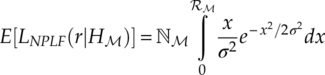
where ![]() is the maximum number of matching centroids for the hypothesis
is the maximum number of matching centroids for the hypothesis ![]() ;. For example, given a piece of QPSK signal, the value of
;. For example, given a piece of QPSK signal, the value of ![]() for different hypotheses would be:
for different hypotheses would be: ![]() BPSK = 2,
BPSK = 2, ![]() QPSK = 4 and
QPSK = 4 and ![]() 8 − PSK = 4. To simplify the analysis, we generalize the analysis to three general scenarios: hypothesis of lower order
8 − PSK = 4. To simplify the analysis, we generalize the analysis to three general scenarios: hypothesis of lower order ![]() ;−, hypothesis of matching model and order
;−, hypothesis of matching model and order ![]() ;0, and hypothesis of higher order
;0, and hypothesis of higher order ![]() ;+. In order to satisfy the conditions
;+. In order to satisfy the conditions ![]() , and
, and ![]() , the reference radius
, the reference radius ![]() 0 should satisfy the condition given in equation (7.32),
0 should satisfy the condition given in equation (7.32),
where αR is the radius factor and αi is the channel gain estimated for modulation ![]() ;(i) . The determination of the radius factor depends on the range of SNR the classifier operates in, and a detailed analysis is given in Zhu and Nandi (2014). An illustration of the classifier is given in Figure 7.2.
;(i) . The determination of the radius factor depends on the range of SNR the classifier operates in, and a detailed analysis is given in Zhu and Nandi (2014). An illustration of the classifier is given in Figure 7.2.
Figure 7.2 Centroid estimation and NPLF classifier.
7.4 Conclusion
In this chapter we present a few blind modulation classification approaches. The first approach combines EM estimation with likelihood-based classifiers. The ML classifier provides an easy implementation of AMC following the EM channel estimation. The minimum likelihood distance classifier is listed as an alternative approach to the ML classifier, which is able to overcome the performance issues associated with the combination of ML-based estimator and ML-based classifier. The minimum distance centroid estimation provides a quick way to estimate channel gain. It is well complemented by the non-parametric likelihood classifier where knowledge of the noise variance is not required during the classification. The classifier also has the advantage that performance degradation in non-Gaussian noise channel is relatively small.
References
- Azzouz, E.E. and Nandi, A.K. (1996) Automatic Modulation Recognition of Communication Signals, Kluwer, Boston.
- Chavali, V.G. and Da Silva, C.R.C.M. (2011) Maximum-likelihood classification of digital amplitude-phase modulated signals in flat fading non-Gaussian channels. IEEE Transactions on Communications, 59 (8), 2051–2056.
- Chavali, V.G. and Da Silva, C.R.C.M. (2013) Classification of digital amplitude-phase modulated signals in time-correlated non-Gaussian channels. IEEE Transactions on Communications, 61 (6), 2408–2419.
- Dobre, O.A., Abdi, A. and Bar-Ness, Y. (2005) Blind Modulation Classification: A Concept Whose Time Has Come. IEEE Sarnoff Symposium on Advances in Wired and Wireless Communication, 18 May 2005, IEEE, pp. 223–228.
- Gao, P. and Tepedelenlioglu, C. (2005) SNR estimation for nonconstant modulus constellations. IEEE Transactions on Signal Processing, 53 (3), 865–870.
- Geoffrey, M. and Peel, D. (2000) Finite Mixture Models, John Wiley & Sons, Inc., New York.
- Meng, X.-L. and Rubin, D.B. (1993) Maximum likelihood estimation via the ECM algorithm: a general framework. Biometrika, 80 (2), 267–278.
- Moon, T.K. (1996) The expectation-maximization algorithm. IEEE Signal Processing Magazine, 13 (6), 47–60.
- Panagiotou, P., Anastasopoulos, A. and Polydoros, A. (2000) Likelihood Ratio Tests for Modulation Classification. Military Communications Conference, 22 October 2000, IEEE, pp. 670–674.
- Sexton, J. (2000) ECM algorithms that converge at the rate of EM. Biometrika, 87 (3), 651–662.
- Soltanmohammadi, E. and Naraghi-Pour, M. (2013) Blind modulation classification over fading channels using expectation-maximization. IEEE Communications Letters, 17 (9), 1692–1695.
- Spooner, C.M. (1996) Classification of Co-channel Communication Signals Using Cyclic Cumulants. Conference Record of the Twenty-Ninth Asilomar Conference on Signals, Systems and Computers, 30 October 1995, IEEE, pp. 531–536.
- Swami, A. and Sadler, B.M. (2000) Hierarchical digital modulation classification using cumulants. IEEE Transactions on Communications, 48 (3), 416–429.
- Tzikas, D.G., Likas, A.C. and Galatsanos, N.P. (2008) The variational approximation for bayesian inference. IEEE Signal Processing Magazine, 25 (6), 131–146.
- Wang, F. and Wang, X. (2010) Fast and robust modulation classification via Kolmogorov–Smirnov test. IEEE Transactions on Communications, 58 (8), 2324–2332.
- Wei, W. and Mendel, J.M. (2000) Maximum-likelihood classification for digital amplitude-phase modulations. IEEE Transactions on Communications, 48 (2), 189–193.
- Wong, M.L.D. and Nandi, A.K. (2008) Semi-blind algorithms for automatic classification of digital modulation schemes. Digital Signal Processing, 18 (2), 209–227.
- Zhu, Z. and Nandi, A.K. (2014) Blind Digital Modulation Classification using Minimum Distance Centroid Estimator and Non-parametric Likelihood Function. IEEE Transactions on Wireless Communications, 13 (8), 4483–4494.