
3
Likelihood-based Classifiers
3.1 Introduction
Likelihood-based (LB) modulation classifiers are by far the most popular modulation classification approaches. The interest in LB classifiers is motivated by the optimality of its classification accuracy when perfect channel model and channel parameters are known to the classifiers (Huang and Polydoros, 1995; Sills, 1999; Wei and Mendel, 2000; Hameed, Dobre and Popescu, 2009; Ramezani-Kebrya et al., 2013).
The common approach of an LB modulation classifier consists of two steps. In the first step, the likelihood is evaluated for each modulation hypothesis with observed signal samples. The likelihood functions are derived from the selected signal model and can be modified to fulfil the need of reduced computational complexity or to be applicable in non-cooperative environments. In the second step, the likelihood of different modulation hypothesizes are compared to conclude the classification decision. Earlier methods of decision making are enabled with a ratio test between two hypothesizes. The requirement of a threshold provides another level of optimization which may provide improved classification performance but also requires more tentative effort to select thresholds. The more intuitive approach of decision making would be to find the maximum likelihood among all candidates. It is much easier to implement and does not require carefully designed thresholds.
In reality, much effort has been made to modify the likelihood approach for lower computational complexity and versatility in non-cooperative environments. In this chapter, we will first present the maximum likelihood (ML) classifier. The alternatives of average likelihood ratio test (ALRT), generalized likelihood ratio test (GLRT) and hybrid likelihood ratio test (HLRT) will be discussed. The last section will be dedicated to the complexity reduction of the likelihood-based classifiers.
3.2 Maximum Likelihood Classifiers
Likelihood evaluation is equivalent to the calculation of probabilities of observed signal samples belonging to the models with given parameters. In a maximum likelihood classifier, with perfect channel knowledge, all parameters are known except the signal modulation. Therefore, the classification process can also be perceived as a maximum likelihood estimation of the modulation type where the modulation type is found in a finite set of candidates.
We will focus on deriving the likelihood function in the AWGN channel while modification of the likelihood function in fading channels and non-Gaussian channels will also be mentioned briefly.
3.2.1 Likelihood Function in AWGN Channels
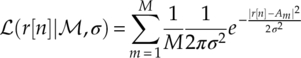
Given that the likelihood of the observed signal sample r[n] belonging to the modulation M is equal to the probability of the signal sample r being observed in the AWGN channel modulated with ![]() , then equation (3.1) holds.
, then equation (3.1) holds.
As we recall the complex form PDF of received signal in AWGN channel, the likelihood function can be found as shown in equation (3.2).
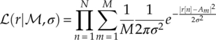
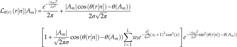
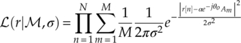
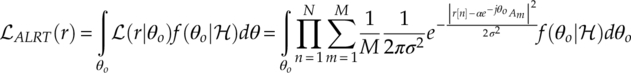
Without knowing which modulation symbol the signal sample r[n] belongs to, the likelihood is calculated using the average of the likelihood value between the observed signal sample and each modulation symbol Am. The joint likelihood given multiple observed samples is calculated with the multiplication of all likelihoods of individual samples, as given in equation (3.3).
For analytical convenience in many cases, the natural logarithm of the likelihood ![]() is used as the likelihood value to be compared in a maximum likelihood classifier [equation (3.4)].
is used as the likelihood value to be compared in a maximum likelihood classifier [equation (3.4)].

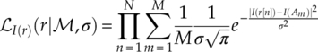
The likelihood, in the meantime, can be derived from probabilities of different aspects of sampled signals. As we have derived the PDF for in-phase segments of the received signal in AWGN channel, the corresponding likelihood function of the in-phase segments of a signal can be found as given in equation (3.5).
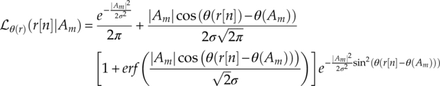
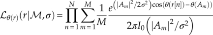
The signal phase is another natural subject of study when applying maximum likelihood classification on M-PSK modulations while M-QAM modulations can also be classified (Shi and Karasawa, 2011). The advantage of using the signal phase solely for likelihood evaluation is highlighted by its robustness in channels where amplitude distortions are exhibited. However, the method is overshadowed by its vulnerability against phase and frequency offsets. Using the PDF of the signal phase in AWGN channel from equation (2.7), the phase likelihood function can be derived as given in equation (3.6).
Owing to the complex form of the likelihood function, different alternative PDFs have been proposed to simplify the phase likelihood function. The von Mises distribution PDF is a much lighter alternative to the PDF given in equation (2.7). The phase likelihood function based on the von Mises PDF is given by equation (3.7).
As mentioned in Chapter 2, the von Mises distribution requires a certain SNR level to be valid. At low SNR level the approximation will deviate from the accurate PDF and a systematic error in likelihood evaluation will lead to inaccurate classification. For this reason, Shi and Karasawa (2012) proposed an approximation to the accurate PDF in equation (2.7) using Gaussian Legendre quadrature rules to replace the error function in equation (3.6) with a finite-range integral (Abramowitz and Stegun, 1964), as shown in equation (3.8),
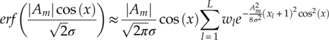
where L is the number of points, ![]() are the weights, and
are the weights, and ![]() are the abscissas of the semi-infinite Gauss–Hermite quadrature rule (Steen, Byrne and Gelbard, 1969). Therefore, the corresponding phase likelihood function using the approximation can be derived by substituting equation (3.8) into equation (3.6) to give equation (3.9).
are the abscissas of the semi-infinite Gauss–Hermite quadrature rule (Steen, Byrne and Gelbard, 1969). Therefore, the corresponding phase likelihood function using the approximation can be derived by substituting equation (3.8) into equation (3.6) to give equation (3.9).
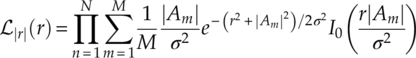
The magnitude likelihood function can be implemented for the classification of M-QAM modulations and M-PAM modulations. The unique advantage of the magnitude likelihood appears when a phase or frequency offset is observed in the transmission channel. As the PDF of signal magnitude in AWGN or fading channel only consists of the magnitude of the transmitted symbols, any rotational shift would not alter the resulting probability evaluation. Using the PDF of signal magnitude in AWGN channel given in equation (2.12), the magnitude likelihood can be found as shown in equation (3.10).
3.2.2 Likelihood Function in Fading Channels
Though the likelihood functions in AWGN channels are the primary subject of research, it would be interesting to derive their variant in fading channels. In this section, channel attenuation and phase shift in both slow and fast fading scenarios are introduced to the ML classifier. The information is used to modify the likelihood function derived for AWGN channels to compensate the added effect from fading channels.
In slow fading channel where amplitude attenuation and phase shift are both considered constant, the modification to the likelihood function is restricted to the transmitted signal symbols. Assume the known or estimated attenuation is α and θo, the symbol Am would endure a shift and result in a new position for ![]() . Substitute the new symbol positions into the likelihood function in equation (3.3), and the likelihood function in slow fading channel with constant amplitude attenuation and phase shift can be found as given in equation (3.11).
. Substitute the new symbol positions into the likelihood function in equation (3.3), and the likelihood function in slow fading channel with constant amplitude attenuation and phase shift can be found as given in equation (3.11).
The likelihood function in fast fading channel is negated here as the collection of parameters needed for the accurate likelihood evaluation is unlikely to be all known to the classifier. The estimation of all the parameters also seems ambitious, which renders the exact likelihood function for the fast fading channel impractical.
3.2.3 Likelihood Function in Non-Gaussian Noise Channels
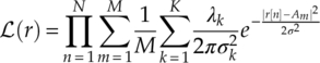
As impulsive noises are common in communication channels, it is important to derive the likelihood function for signals in non-Gaussian noise channels with impulsive noises. Middleton’s Class A model and the SαS model, though being relatively accurate, have many parameters in their PDFs and characteristic functions. Considering the extra mismatch which may be introduced in the process of estimation these parameters, the GMM model is adopted as the bases for the likelihood function in non-Gaussian noise channels. From equation (2.28), assuming the probability λk and variance ![]() for total number of K Gaussian components are known or estimated, the likelihood function can be found as given in equation (3.12).
for total number of K Gaussian components are known or estimated, the likelihood function can be found as given in equation (3.12).
3.2.4 Maximum Likelihood Classification Decision Making
Having established the likelihood functions in different channel scenarios from different signal segments, the decision making in an ML classifier becomes rather straightforward. Assuming a pool with finite number I modulation candidates ![]() , among which hypothesis
, among which hypothesis ![]()
![]() ;(i) of each modulation
;(i) of each modulation ![]() ;(i) is evaluated using estimated channel parameters
;(i) is evaluated using estimated channel parameters ![]() and a suitable likelihood function to obtain its likelihood evaluation
and a suitable likelihood function to obtain its likelihood evaluation ![]() (r|
(r|![]()
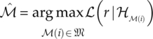
![]() ;(i)). With the all the likelihood values collected the decision is made simply by finding the hypothesis with the highest likelihood [equation (3.13)].
;(i)). With the all the likelihood values collected the decision is made simply by finding the hypothesis with the highest likelihood [equation (3.13)].
The entire process of the ML classification is illustrated in Figure 3.1.
Figure 3.1 Maximum likelihood classifier in fading channel with AWGN noise.
3.3 Likelihood Ratio Test for Unknown Channel Parameters
3.3.1 Average Likelihood Ratio Test
The issue of an unknown parameter in an ML classifier is pivotal as the likelihood function is unable to handle any missing parameter. The average likelihood ratio test (ALRT) is one way to overcome such limitation of an ML classifier. Polydoros and Kim were the first to apply ALRT to modulation classification (Polydoros and Kim, 1990), which was later adopted by Huang and Polydoros (1995), Beidas and Weber (1995), Sills (1999), Hong and Ho (2000). Different from the ML likelihood function, the ALRT likelihood function replaces unknown parameters with the integral of all their possible values and their corresponding probabilities. An example of ALRT likelihood function with unknown constant carrier phase offset is given by equation (3.14),
where ![]() ALRT(r) is the updated ALRT likelihood,
ALRT(r) is the updated ALRT likelihood, ![]() (r|θo) is the likelihood given phase offset of θo, and f(θo|
(r|θo) is the likelihood given phase offset of θo, and f(θo|![]() ) is the probability of constant phase offset θo under modulation hypothesis
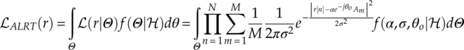
) is the probability of constant phase offset θo under modulation hypothesis ![]() . Other channel parameters such as noise variance σ2 and channel gain α can also be treated individually as unknown parameters with their PDF or as a group of unknown parameters with their joint probability, as shown in equation (3.15),
. Other channel parameters such as noise variance σ2 and channel gain α can also be treated individually as unknown parameters with their PDF or as a group of unknown parameters with their joint probability, as shown in equation (3.15),
where Θ is the collection of unknown parameters. While ![]() (r|θo) is known to the classifier, f(Θ|
(r|θo) is known to the classifier, f(Θ|![]() ) depends on the definition of prior probability of unknown parameters. The common assumption of prior PDFs of different parameters is shown in equations (3.16)–(3.18),
) depends on the definition of prior probability of unknown parameters. The common assumption of prior PDFs of different parameters is shown in equations (3.16)–(3.18),
where channel gain α is given a normal distribution with mean μα, variance ![]() , noise variance is given a Gamma distribution with shape parameter aσ and scale parameter bσ, and phase offset is given a normal distribution with mean
, noise variance is given a Gamma distribution with shape parameter aσ and scale parameter bσ, and phase offset is given a normal distribution with mean ![]() and variance
and variance ![]() . All the additional parameters associated with PDF of channel parameters are often called hyperparameters. The estimation of hyperparameters is not discussed in this book. Suitable schemes have been proposed by Roberts and Penny using a variational Bayes estimator (Roberts and Penny, 2002).
. All the additional parameters associated with PDF of channel parameters are often called hyperparameters. The estimation of hyperparameters is not discussed in this book. Suitable schemes have been proposed by Roberts and Penny using a variational Bayes estimator (Roberts and Penny, 2002).
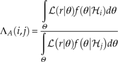
The likelihood ratio test required for the classification decision making is conducted with the assistance of a threshold γA. The actual likelihood ratio is calculated as given in equation (3.19), where the classification result is given using the conditional equation (3.20).
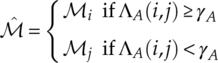
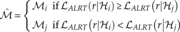
An easy assignment of the ratio test threshold is to define all thresholds to be one. The decision making becomes a simple process of comparing the average likelihood of two hypotheses [equations (3.21)].
Using the same assignment, the maximum likelihood decision making can also be applied using equation (3.13) with the likelihood function with average likelihood.
3.3.2 Generalized Likelihood Ratio Test
It is not difficult to see that the ALRT likelihood function has a much more complex form when unknown parameters are introduced. The requirement of underlining models for unknown parameters confirms that successful classification depends on the accuracy of the models. Consequently, if an accurate model is not available, the method becomes suboptimal and only an approximation to the optimal ALRT classifier. The additional requirement of estimation hyperparameters adds another level of complexity and inaccuracy to the overall performance of the ALRT classifier. It is also the fact that the likelihood function is more complex with added integration operations.
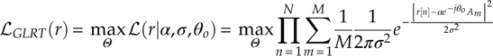
For the above reasons, Panagiotou, Anastasopoulos and Polydoros proposed the generalized likelihood ratio test (GLRT) as an alternative (Panagiotou, Anastasopoulos and Polydoros, 2000). The GLRT in essence is a combination of a maximum likelihood estimator and a maximum likelihood classifier. The likelihood function, unlike the ALRT, replaces the integration of unknown parameters with a maximization of the likelihood over a possible range for the unknown parameters. The likelihood function of the GLRT method is given by equation (3.22).
When multiple unknown channel parameters are presented, the maximum become a process over multiple parameters. There is a favourable order of maximization when channel gain, noise variance and phase offset are all unknown. As recommended in our previous research (Zhu, Nandi and Aslam, 2013), it is easier to obtain an unbiased ML estimation of the phase offset before channel gain and noise variance. Noise variance is normally best to be estimated when all the rest of channel parameters are accurately estimated.
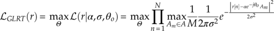
Panagiotou et al. (2000) also included another maximization step to eliminate the effect of averaging the likelihood of the signal samples belonging to different modulation symbols, as shown in equation (3.23).
The complexity is notably further reduced. However, the classifier based on the modified GLRT likelihood function now becomes biased in both low SNR and high SNR scenarios. Assume the modified GLRT likelihood function is used to classify among 4-QAM and 16-QAM signals. At low SNR, when signals are well spread, a 4-QAM modulated signal is always more likely to produce a higher likelihood if using 16-QAM as hypothesis, because the 16-QAM has more symbols and they are more densely populated under the assumption of unit power. At high SNR, when signals are tight around the transmitted symbol, the maximization of the likelihood through channel gain is likely to scale the 16-QAM alphabet such that four central symbols in the alphabet will be overlapping with the alphabet of the 4-QAM modulation. Such a phenomenon observed in nested modulations produces an equal likelihood between low-order modulations and high-order modulations when low-order modulations are being classified. Therefore, the method is clearly biased for high-order modulations in most scenarios.
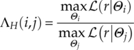
The actual likelihood ratio is calculated as follows [equation (3.24)],
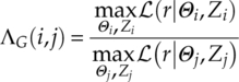
where Zi and Zj define the membership of each observed sample with respect to modulation symbols.
3.3.3 Hybrid Likelihood Ratio Test
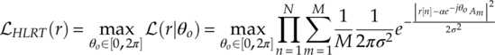
While the GLRT likelihood function provides alternative to ALRT, the fact that it is a biased classifier, as discussed in the previous section, makes it unsuitable for modulation with nested modulations (e.g. QPSK, 8-PSK; 16-QAM, 64-QAM). For this reason, Panagiotou et al. (2000) proposed another likelihood ratio test named hybrid likelihood ratio test (HLRT). In the original publication, the HLRT was suggested as an LB classifier for unknown carrier phase offset. The likelihood in HLRT is calculated by averaging over the transmitted symbols and then maximizing the resulting likelihood function (LF) with respect to the carrier phase. The likelihood function is thus derived as shown in equation (3.25).
It is clear that the HLRT LF calculates the likelihood of each signal sample belonging to each alphabet symbol. Therefore, the case where a nested constellation creates biased classification does not existence. In addition, the maximization process replaces the integral of the unknown parameters and their PDFs for much lower analytical and computational complexity.
The decision making of the HLRT approach follows the same rules as the ALRT and GLRT approach where a threshold γH is required for the ratio test to optimize the classification accuracy. The ratio test becomes the maximum likelihood classifier when the threshold is set to one.
The actual likelihood ratio is calculated as follows [equation (3.26)].
3.4 Complexity Reduction
It is known that the ML classifier has the drawback of high computational complexity. This is mostly due to the need for calculation of natural logarithms in the likelihood function and the increased demand for additional signal samples. Many researchers have recognized the challenge and provided different approaches to reduce the complexity of the ML classifier.
3.4.1 Discrete Likelihood Ratio Test and Lookup Table
Xu, Su and Zhou proposed a fast likelihood function through offline computation (Xu, Su and Zhou, 2011). As pointed out in their work, most of the complexity in an ALRT classifier is contributed by the massive integration, multiplication and exponent arithmetic. Aiming to not degrade the performance of the ALRT classifier, they developed the discrete likelihood ratio test (DLRT) with the addition of a lookup table (LUT). The first step of the classification framework is to build a storage table containing the likelihood of each modulation quantized to a finite set. The quantization of the storage table is done by dividing the continuous complex plane into a P × Q grid with a uniform partition strategy. The other dimension of quantization is done for the noise variance σ2 with U intervals. When a signal sample r[n] is sampled, the complex sample is first mapped to its in-phase component xp and quadrature component yq indexed by p and q. The log-likelihood of this sampling belonging to the hypothesis modulation is found from a cell Ti(p, q, u) from the LUT for modulation i. The table cell itself is calculated using the following equation (3.27),
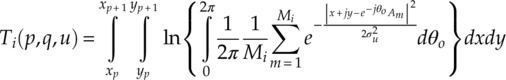
where Mi is the size of the alphabet set of modulation i, and θo is the unknown carrier phase. The subsequent steps of the DLRT and LUT classifier are the same as those in an ALRT classifier.
The complexity and accuracy analysis provided suggests that the classification performance is largely associated with the level of quantization. With higher levels of quantization resolution, the error introduced by mismatching between received signal sample and mapped signal sample along with estimated noise variance and mapped noise variance can be minimized. The price for the increased quantization resolution is solely inflicted as the demand for much larger memory to store the recalculated storage tables.
3.4.2 Minimum Distance Likelihood Function
Wong and Nandi proposed to remove the exponential arithmetic in ML likelihood function with a simple Euclidean distance between a received signal sample and its nearest modulation symbol (Wong and Nandi, 2008). The minimum distance likelihood function (MDLF) is easily given by equation (3.28).
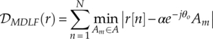
Unlike the LB methods, the decision making is based on finding the modulation hypothesis with the minimum distance.
The obvious advantage of the minimum distance classifier is its low complexity. However, the main drawback is likewise easy to spot. Given a group of well spread signal samples, it is always easier to find a smaller distance when there is a greater number of densely populated centroids. Therefore higher-order modulations are always favoured by the classifier.
3.4.3 Non-Parametric Likelihood Function
Zhu and Nandi recently proposed a non-parametric likelihood function (NPLF) (Zhu and Nandi, 2014). The initial goal was to obtain the likelihood evaluation without a specific signal distribution as well as without the knowledge of the noise variance. In addition, the NPLF also achieves a very low computation complexity. The NPLF function is defined as shown in equation (3.29),
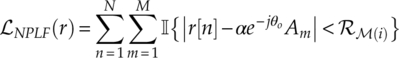
which evaluates the cumulative distribution in a set of regions defined by the modulation symbol and a radius factor ![]() . The calculation of the likelihood is enabled with an indicator function
. The calculation of the likelihood is enabled with an indicator function ![]() which outputs a value of 1 if the input is true and 0 if the input is false. More details of the NPLF function are given in Chapter 7, where it is employed for blind modulation classification.
which outputs a value of 1 if the input is true and 0 if the input is false. More details of the NPLF function are given in Chapter 7, where it is employed for blind modulation classification.
3.5 Conclusion
In this chapter, we have examined different likelihood-based modulation classifiers. The maximum likelihood method is first presented as the optimum classifier with the requirement of known channel state information. Its likelihood function is given in equation (3.3) and the decision making is established in equation (3.13). The assumption of perfect channel knowledge is relaxed by the subsequent ALRT, GLRT and HLRT classifiers. They all consider one or two channel parameters as being unknown. Among these classifiers, the likelihood function of ALRT classifier [equation (3.14)] is the most complex one where multiple integral and exponential operations are need. The GLRT likelihood function has a much simpler form but a biased classification performance. The HLRT presents an option where the complexity and classification performance has a better balance. Other approaches to reduce the complexity of a maximum likelihood classifier are presented in the last part of the chapter.
References
- Abramowitz, M. and Stegun, I. (1964) Handbook of Mathematical Functions: With Formulas, Graphs, and Mathematical Tables. Dover Publications, Mineola, New York.
- Beidas, B.F. and Weber, C. (1995) Higher-order correlation-based approach to modulation classification of digitally frequency-modulated signals. IEEE Journal on Selected Areas in Communications, 13 (1), 89–101.
- Hameed, F., Dobre, O.A. and Popescu, D. (2009) On the likelihood-based approach to modulation classification. IEEE Transactions on Wireless Communications, 8 (12), 5884–5892.
- Hong, L. and Ho, K.C. (2000) BPSK and QPSK Modulation Classification with Unknown Signal Level. Military Communications Conference, Los Angeles, CA, USA, 22 October 2000, pp. 976–980.
- Huang, C.Y. and Polydoros, A. (1995) Likelihood methods for MPSK modulation classification. IEEE Transactions on Communications, 43 (2), 1493–1504.
- Panagiotou, P., Anastasopoulos, A. and Polydoros, A. (2000) Likelihood Ratio Tests for Modulation Classification. Military Communications Conference, Los Angeles, CA, USA, 22 October 2000, pp. 670–674.
- Polydoros, A. and Kim, K. (1990) On the detection and classification of quadrature digital modulations in broad-band noise. IEEE Transactions on Communications, 38 (8), 1199–1211.
- Ramezani-Kebrya, A., Kim, I.-M., Kim, D.I. et al. (2013) Likelihood-based modulation classification for multiple-antenna receiver. IEEE Transactions on Communications, 61 (9), 3816–3829.
- Roberts, S.J. and Penny, W.D. (2002) Variational bayes for generalized autoregressive models. IEEE Transactions on Signal Processing, 50 (9), 2245–2257.
- Shi, Q. and Karasawa, Y. (2011) Noncoherent maximum likelihood classification of quadrature amplitude modulation constellations: simplification, analysis, and extension. IEEE Transactions on Wireless Communications, 10 (4), 1312–1322.
- Shi, Q. and Karasawa, Y. (2012) Automatic modulation identification based on the probability density function of signal phase. IEEE Transactions on Communications, 60 (4), 1–5.
- Sills, J.A. (1999) Maximum-likelihood Modulation Classification for PSK/QAM. Military Communications Conference, Atlantic City, NJ, 31 October 1999, pp. 217–220.
- Steen, N.M., Byrne, G.D. and Gelbard, E.M. (1969) Gaussian quadratures for the integrals. Mathematics of Computation, 23 (107), 661–671.
- Wei, W. and Mendel, J.M. (2000) Maximum-likelihood classification for digital amplitude-phase modulations. IEEE Transactions on Communications, 48 (2), 189–193.
- Wong, M.L.D. and Nandi, A.K. (2008) Semi-blind algorithms for automatic classification of digital modulation schemes. Digital Signal Processing, 18 (2), 209–227.
- Xu, J.L., Su, W. and Zhou, M. (2011) Likelihood-ratio approaches to automatic modulation classification. IEEE Transactions on Systems, Man, and Cybernetics, Part C (Applications and Reviews), 41 (4), 455–469.
- Zhu, Z. and Nandi, A.K. (2014) Blind Digital Modulation Classification using Minimum Distance Centroid Estimator and Non-parametric Likelihood Function. IEEE Transactions on Wireless Communications, doi: 10.1109/TWC.2014.2320724, 1–12.
- Zhu, Z., Nandi, A.K. and Aslam, M.W. (2013) Approximate Centroid Estimation with Constellation Grid Segmentation for Blind M-QAMClassification. Military Communications Conference, San Diego, CA, USA, 18 November 2013, pp. 46–51.