
15
THE YULE–WALKER EQUATIONS AND THE PARTIAL AUTOCORRELATION FUNCTION
15.1 BACKGROUND
In this chapter, the last tools are developed in order to justify modeling any ARMA(m,l) model with an AR(m) filter: The Yule–Walker equations [and the R functions ar.yw() and ar.mle()], the partial autocorrelation function and plot [and the R function pacf()], and the spectrum for ARMA(m,l) models as well as the relationship between the spectrum and the impulse response function (this will not be particularly useful for modeling, but it is too cool not to mention, and does not take up much space).
15.2 AUTOCOVARIANCE OF AN ARMA(M,L) MODEL
15.2.1 A Preliminary Result
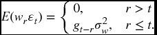
The autocovariance function, with the derivation of the impulse response function, can be viewed from a very different perspective. Recall that there is an interest in computing things like E(wrϵt), but now it has been established that ϵt is a linear combination of all white noise components up to, and including, time t. Recall also that E(wjwk) = 0, unless j = k, in which case E(w2j) = σw2.
So ![]() and
and ![]() . The only nonzero component of this infinite series is when r = t − j, if that is possible (if r > t, this is not possible). Therefore:
. The only nonzero component of this infinite series is when r = t − j, if that is possible (if r > t, this is not possible). Therefore:
15.2.2 The Autocovariance Function for ARMA(m,l) Models
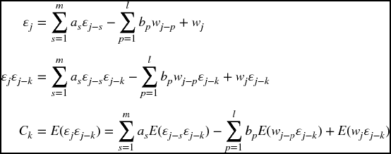
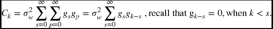
Recall that the autocovariance, Ck = C− k = E(ϵj, ϵj ± k). A few definitions and the application of the previous results yields
Suppose k = 0,
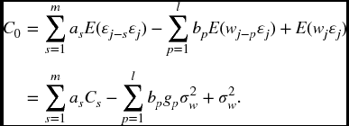
Suppose k > 0
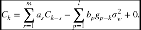
In the second summation gp − k = 0 when k > p.
15.3 AR(M) AND THE YULE–WALKER EQUATIONS
15.3.1 The Equations
For any AR(m) model, bp = 0, for all p. In this special case, the previous equations reduce to the Yule–Walker equations (replacing parameters with estimates):
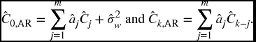
In other words, if the autocovariance function has been computed, and it is assumed the model is ARMA(m,0), it is possible to estimate the unknown values, ![]() by solving a linear system of equations.
by solving a linear system of equations.
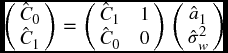
The AR(1) model, using the Yule–Walker equations, produces the system ![]() and
and ![]() . From the acf() function, the values
. From the acf() function, the values ![]() and
and ![]() can be computed, which will allow estimation of a1 and σ2w using the Yule–Walker equations. In matrix form, the system is
can be computed, which will allow estimation of a1 and σ2w using the Yule–Walker equations. In matrix form, the system is
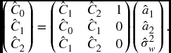
Similarly, for an AR(2) model, m = 2 , there are three equations in three unknowns:
In matrix form [recall that Ck = C− k and acf() is used to estimate values], the system is
15.3.2 The R Function ar.yw() with an AR(3) Example
An R function is available for solving the Yule–Walker equations, ar.yw(). Pass any sequence of errors or residuals to the function and the function will solve a sequence of models, AR(1)…AR(m) and pick the best model using the criterion of minimizing AIC. It should be noted that the Yule–Walker estimates are not maximum likelihood estimates, so that AIC is only approximated.
This useful R function will be demonstrated by first simulating a sequence of AR(3) errors and comparing the fitted models AR(0),…, AR(6). Subtle distinctions are important. Because the true model is known to be AR(m), BIC should be used to select the best model. Hypothesis testing will also be used as an alternative method of model selection.
The simplest way to be assured that the AR(3) model is stationary is to begin with the roots, being assured, they are all less than one in magnitude.
# Simulating 2000 AR(3) errors
error <- arima.sim(n = 2000, list(ar=c(1.4,-0.31, -0.126)),sd = 3.0)
plot(1:2000,error)
lines(1:2000, error)
abline(0,0)
title(“AR(3) errors, n= 2000”)
This produces Figure 15.1.
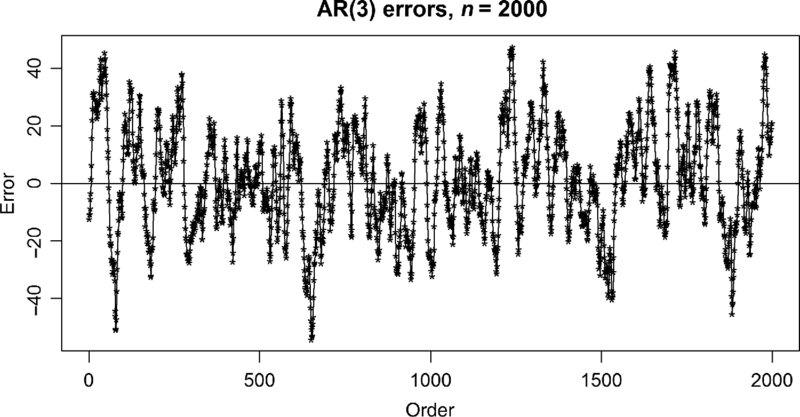
FIGURE 15.1 A sequence of errors.
The next step is to use the function ar.yw() and understand the various information produced by the function:
z <- ar.yw(error), names(z)[1] ``order" ``ar" ``var.pred" ``x.mean" ``aic"
[6] ``n.used" ``order.max" ``partialacf" ``resid" ``method"
[11] ``series" ``frequency" ``call" ``asy.var.coef"The most important command, following up on ar.yw() is z$aic
| 0 | 1 | 2 | 3 | 4 | 5 |
| 7218.086359 | 632.339343 | 33.650225 | 0.000000 | 0.941779 | 2.716482 |
| 6 | 7 | 8 | 9 | 10 | 11 |
| 4.697557 | 6.140760 | 6.326040 | 8.076309 | 9.674298 | 11.588804… |
This is a common format for AIC values. With AIC (or BIC), the values themselves are unique only up to a common constant, and it is the minimum value and differences that are important. Therefore, all values are frequently reported as differences from the minimum value. Using AIC, the AR(3) model is identified as the best, and the AR(4) model is only slightly worse (0.941779 greater). In some sense, the AR(3) model appears just 1.6 (exp[0.941779/2] = 1.6) times more believable than the AR(4) model, not a large difference.
Some other components of this output often used are
- The order, m, of the model chosen by AIC: z$order 3.
- The values of
 for the chosen order: z$ar 1.4133773 -0.3124876 -0.1329180.
 - The estimate
 (recall, σ2w = 9): z$var.pred 8.728231.
In some cases, there is a desire to find ![]() and/ or
and/ or ![]() for a different model. In that case, the command z <- ar.yw(error, aic = FALSE, order.max = m) will ignore AIC (aic = FALSE) and force the fitting of some specified order m. [Recall, many other things can be learned using help(ar.yw)].
for a different model. In that case, the command z <- ar.yw(error, aic = FALSE, order.max = m) will ignore AIC (aic = FALSE) and force the fitting of some specified order m. [Recall, many other things can be learned using help(ar.yw)].
15.3.3 Information Criteria-Based Model Selection Using ar.yw()
For the previous simulation, the correct model is to be picked from a list of candidate models. Therefore, in this circumstance, BIC is preferred to AIC for model selection (Aho et al., 2014). As with many previous modeling exercises, a model selection table is developed.
For each candidate model, AR(0) to AR(7), the command ar.yw(error, aic = FALSE, order.max = m) can be used to fit a specified order [For m = 0, var(error) was used to estimate ![]() ]. Because information criteria assumes maximum likelihood estimates, a slightly different command can be used to get just those values—z <- ar.mle(error, aic = FALSE, order.max = m). The model selection table is produced using ar.mle() to obtain
]. Because information criteria assumes maximum likelihood estimates, a slightly different command can be used to get just those values—z <- ar.mle(error, aic = FALSE, order.max = m). The model selection table is produced using ar.mle() to obtain ![]() .
.
It is not obvious precisely how AIC is computed for ar.yw(), nor is BIC computed. However, a reasonable estimate would be ![]() , using ar.mle() to estimate σ2w. The estimated BIC values in Table 15.1 were computed in this manner.
, using ar.mle() to estimate σ2w. The estimated BIC values in Table 15.1 were computed in this manner.
TABLE 15.1 Model Selection Using Information Criteria (![]() )
)
| Model | ΔAIC | ≈ BIC | ≈ ΔBIC | |
| m = 0 | 322.82 | 7218.09 | 11,554.19 | 7202.44 |
| 1 | 11.97 | 632.34 | 4972.41 | 620.66 |
| 2 | 8.87 | 33.65 | 4380.55 | 28.80 |
| 3 | 8.71 | 0.00 | 4351.75 | 0.00 |
| 4 | 8.70 | 0.94 | 4357.05 | 5.30 |
| 5 | 8.70 | 2.72 | 4364.65 | 12.90 |
| 6 | 8.70 | 4.70 | 4372.25 | 20.50 |
| 7 | 8.70 | 6.14 | 4379.85 | 28.80 |
The choice of ar.yw() versus ar.mle() for estimation of σ2w was of no impact [The AIC values here match the earlier ar.yw()-based values almost perfectly]. Because ar.mle() may run slow or even fail to converge for large sets of data, and because the derivation for the Yule–Walker equations has been given and the derivation of the maximum likelihood approach is beyond this book, ar.yw()will be the default method for the rest of the book.
The results from Table 15.1 correctly identify the AR(3) model as the model that generated that data. Of course, in this case, the choice is obvious and both AIC and BIC make the same correct choice. The estimated variance drops substantially for each order up to and including order 3. However, after that there is no further drop in variance, so further increases in complexity gain nothing.
15.4 THE PARTIAL AUTOCORRELATION PLOT
15.4.1 A Sequence of Hypothesis Tests
Let ![]() be the estimate of
be the estimate of ![]() for the model AR(m). It is known that (Box et al., 2008, p. 70)
for the model AR(m). It is known that (Box et al., 2008, p. 70) ![]() if the true model has order less than m. Therefore
if the true model has order less than m. Therefore ![]() is standard normal if the order is less than m and can be treated as a test statistic for “Ho: the order is less than m” versus “Ha: the order is at least m.”
is standard normal if the order is less than m and can be treated as a test statistic for “Ho: the order is less than m” versus “Ha: the order is at least m.”
Table 15.2 continues with the last data, adding this computed z-score and the p-value associated with the z-score.
TABLE 15.2 A Sequence of Tests for the Order (![]() )
)
| AR(m) | z | p-Value | ||
| m = 1 | 0.9813 | 0.9808 | 43.86 | ≈ 0.0000 |
| 2 | −0.5093 | −0.5089 | −22.76 | ≈ 0.0000 |
| 3 | −0.1329 | −0.1335 | −5.97 | ≈ 0.0000 |
| 4 | 0.0223 | 0.0225 | 1.01 | 0.3124 |
| 5 | 0.0106 | 0.0109 | 0.49 | 0.6242 |
| 6 | 0.0031 | 0.0032 | 0.14 | 0.8886 |
| 7 | −0.0167 | −0.0161 | 0.72 | 0.4716 |
It seems clear that the correct order is 3 from these hypothesis tests. Put more precisely, the data suggests that an order of at least 3 is required, but there is no evidence that an order higher than 3 is required. In this case, AIC, BIC, and hypothesis tests produce identical and unambiguous model selection. Table 15.2 also shows how similar the estimates provided by ar.yw() and ar.mle() often are, at least for large data sets.
15.4.2 The pacf() Function—Hypothesis Tests Presented in a Plot
If the values ![]() for m = 1,2,3,… are plotted versus m, with lines at
for m = 1,2,3,… are plotted versus m, with lines at ![]() , the display becomes a visual representation of the above hypothesis tests. When
, the display becomes a visual representation of the above hypothesis tests. When ![]() falls far outside the lines
falls far outside the lines ![]() , there is evidence that the model is at least of order m; when the values begin to fall far inside the lines, the indications are that the order is no higher than the last large spike.
, there is evidence that the model is at least of order m; when the values begin to fall far inside the lines, the indications are that the order is no higher than the last large spike.
It is clear from Figure 15.2, which is the information from Table 15.2 in a slightly different format, that the errors appear to be of order m = 3.
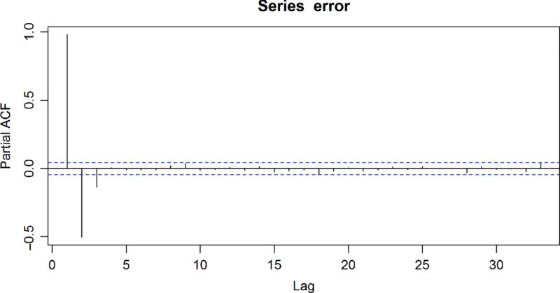
FIGURE 15.2 The pacf() plot for the previously simulated errors.
The autocorrelation plot and the partial autocorrelation plot have complimentary roles. For an AR(m) process, the partial autocorrelation plot is expected to have m significant spikes while the spikes in the autocorrelation plot will slowly decay. For an MA(l) process, the autocorrelation plot will have l distinct spikes, but the partial autocorrelation plots will exhibit a low decay (Box et al., 2008, p. 75; Kitagawa, 2010, pp. 87–89). Compare the plots for the following errors:
AR_error <- arima.sim(n = 500, list(ar=c(0.5,0.4)), sd = 2.0)
MA_error <- arima.sim(n = 500, list(ma=c(0.5,0.4)), sd = 2.0)
The pacf() and acf() plots for these errors are displayed in Figure 15.3.
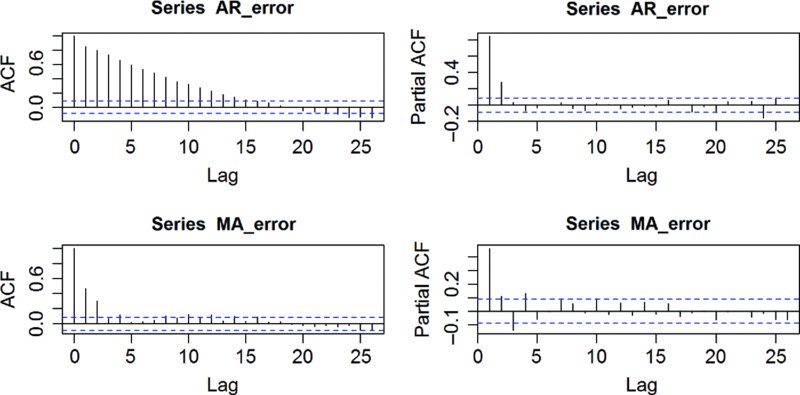
FIGURE 15.3 MA(l) versus AR(m), acf() and pacf() plots.
As can be seen from Figure 15.3, the theory often finds the data quite uncooperative.
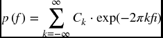
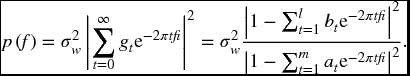
15.5 THE SPECTRUM FOR ARMA PROCESSES
Recall that the spectrum is defined as
The expansion ![]() is now available using the impulse response function.
is now available using the impulse response function.
Note, as before gp = 0, for p < 0. After some preliminary manipulations, Ck will be found to be a function of the gj values, and these will be substituted into the above expression for p(f). A surprising and elegant result will follow:
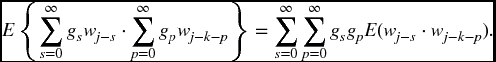
Recall that E(wrwt) = σ2w, when r = t, and E(wrwt) = 0, when r ≠ t. Therefore, all terms in the above expression are zero unless p = k − s. So
Therefore ![]() .
.

Recall that gk − s = 0 for k − s < 0.
Now let p = k − s (Figure 15.4).
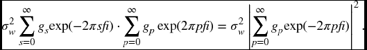
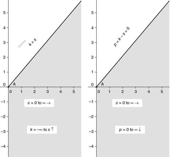
FIGURE 15.4 Change of variable, p = k − s.
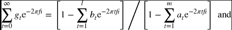
If this were not interesting enough in itself, recall that g(B) = a(B)− 1b(B). Furthermore, the method of equating like coefficients to derive all gj for j = 0,1,2,… is valid when B is replaced with exp( − 2πtfi). So
15.6 SUMMARY
Chapter 14 introduced a substantial generalization and integration of the ARMA(m,l) family of nonwhite noise error. In Chapter 14, the impulse response function was developed, as was an informal argument that ARMA(m,l) = AR(∞). In Chapter 15, these ideas were extended so that it was shown that a broad number of tools are possible for examining AR(m) models. It has been shown that, for all AR(m) models, the Yule–Walker equations implemented in R with the function ar.yw() allow for estimation of all the values a1…am and σ2w, with model selection based on AIC. Also, the R function pacf() provides model selection based on a sequence of hypothesis tests presented in a graph that has the property that, for any AR(m) model, the graph will have exactly m spikes. It is also hinted, in Chapter 13, that a filter can be developed for any AR(m) model.
Given the wealth of tools for AR(m) models and the lack of tools for MA(l) models, it may not be hard to guess where the next chapter leads.
EXERCISES
-
Show that, for complex numbers, if f = g/h, then
 (a brute force approach involves defining g and h quite generally and showing the result).
 -
Using pacf() and ar.yw() or ar.mle(), verify that the following models from Chapter 13 are, indeed, quite plausibly AR(1). That is, the residuals are AR(1) after fitting the signal: (i) the logging data, (ii) the global warming data, (iii) the Semmelweis data, (iv) the adjusted NYC temperatures, (iv) Boise riverflow data (with at least three pairs of periodic functions).
-
Simulate 400 AR(1) errors with a = 0.8 and σ = 2.0. Use ar.yw() to get the estimates of a and σ and verify that these estimates satisfy the Yule–Walker equations.
-
Repeat Exercise 3 for an AR(2) model with a1 = 0.7 and a2 = −0.3.
-
Simulate MA(2) data with b1 = −0.5, b2 = 0.1, and n = 500. Find the autocorrelation plot and partial autocorrelation plot. Do the plots follow the pattern suggested in this chapter? Explain.
-
Simulate AR(2) data with a1 = 0.7, a2 = −0.4, and n = 400. Find the autocorrelation plot and partial autocorrelation plot. Do the plots follow the pattern suggested in this chapter? Explain.
-
Give the matrix representation for the Yule–Walker equations for AR(4).
-
Using (1 − .7B)(1 + [0.1 − 0.1i]B)(1 − [0.1 + 0.1i]B)ϵn = wn
- Find the values for a1, a2, and a3.
- Why do we know this is a stationary process?
- Write out the Yule–Walker equations for AR(3).
- Simulate n = 500 observations from this model.
- Using ar.yw() [or ar.mle()] and pacf(), assess whether the data appears to be AR(3).
- Using ar.yw(x, aic = FALSE, order.max = 3) verify that the values computed with this routine satisfy the Yule–Walker equations (expect an unavoidable round-off error on your part).
-
Consider the following three AR(2) (quadratic) problems of the form

Case 1: c1 = 0.7, c2 = 0.6
Case 2: c1 = 0.7, c2 = −0.6
Case 3: c1 = 0.6 − 0.3i, c2 = 0.6 + 0.3i
in each case, complete the following steps:
- Determine the coefficients a1 and a2.
- Simulate the data according to this model, with n = 800.
- Fit models A(1)…AR(4) to the data using the ar.yw() or ar.mle().
- Complete a table that uses AIC, BIC, and hypothesis testing to select the best model.
- Verify, using pacf(), that the partial autocorrelation plot produces similar results to your table for the hypothesis testing part of the table. Explain what you are looking to in your table and the pacf () plot.
-
Show that for MA(2), for all k, |Rk| < 1 for any choice of b1 and b2. In other words, it is always “well behaved.”
-
Consider the MA(2) model ϵj = −b2wj − 2 − b1wj − 1 + wj with invertibility conditions (i) b1 + b2 < 1, (ii) b2 − b1 < 1, and (iii) |b2| < 1.
Pick choices of b1 and b2 that violate each condition, but only one condition at a time. In each case, show b(B) = 0 has one or more roots inside the unit circle. Since b(B) = 0 is a quadratic, it should be possible to do this easily.