
19
CHRISTOPHER TENNANT/BEN CROSBY WATERSHED DATA
19.1 BACKGROUND AND QUESTION
This data, due to graduate student Christopher Tennant and Professor Ben Crosby of the Idaho State University Geosciences department, is a measure of water flow rates at 12 watersheds in Idaho. The watersheds are contained within three different elevation ranges, representing different types of precipitation (low elevations have precipitation dominated by rain, higher elevations have snow-dominated precipitation, and the mid-elevations have mixed precipitation). The data is in the Tennant folder on the data disk (this data is not in DataMarket):
- Low (rain) elevation: Baker Gulch, Gregory Creek, Rice Creek, Rock Creek.
- Mid (mixed) elevation: Boulder Creek, Little Goose Creek, North Fork Slate Creek, Slate Creek.
- High elevation (snow): Beaver Creek, Frenchman Creek, Salmon River, Smiley Creek.
The final measurement, which was taken for 1054 days (2.89 years) was normalized discharge (the volume of discharge per unit of time divided by the surface area of the watershed). The final units are millimeters per day. Normalized discharge reveals the amount of water contributed per unit area from a drainage basin and provides a convenient measure for comparing water flux from watersheds of different size.
This is a preliminary analysis of the data and the interest is in whether the three regimes behave differently. In the main analysis, an exploration of whether the low and mid-elevations produce different patterns is undertaken. In the exercises, a similar analysis of the low versus high elevations is undertaken.
A couple of methods will be used to compare fit within groups to fit between groups. The general idea is that each watershed is different, but that if the classification into low, mid, and high elevations is important, the watersheds within a group will be more alike than they would be to watersheds in other groups.
19.2 LOOKING AT THE DATA AND FITTING FOURIER SERIES
19.2.1 The Structure of the Data
As with much of the data found in the real world, there is a distinct right skew, and a logarithmic transformation is desirable. In this case, the transformation is z = log e(y + 0.001), where y values are the original measurements. In a couple cases, the smallest observation is 0, and the logarithmic transformation cannot be applied to 0. In order to apply the logarithmic transformation, an amount must be added to each observation—0.001 was chosen.
19.2.2 Fourier Series Fits to the Data
The first fit to the data will be a saturated model (365 days), so that the residuals can be diagnosed for AR(m) structure. For all parts of the analysis, the more alike watersheds within a regime are, the more promising the analysis. In this part of the analysis, it will be great if all watersheds, within an elevation class, have similar AR(m) structure.
The mid- and low-elevation fits look very different. The peaks in the mid-elevation watershed rates (Figure 19.1) are more symmetric, while the low-elevation watersheds have slow buildups to a peak, then sharp declines (Figure 19.2).
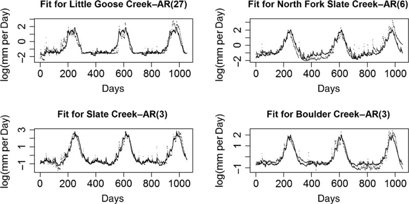
FIGURE 19.1 The initial fits for the mid-elevation watersheds.
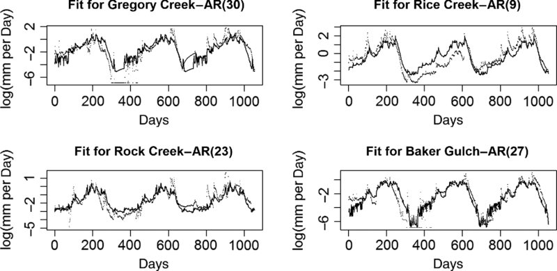
FIGURE 19.2 The initial fits for the low-elevation watersheds.
Three of the four low-elevation (Figure 19.2) watersheds had a very dry period in the first full low phase in the data.
Although the residuals from many of the sites are quite complex, as high as AR(30), the residuals from the regressions between sites might not display the same degree of complexity.
19.2.3 Connecting Patterns in Data to Physical Processes
Why are the residuals so complex? Although the complexity of the residuals is partly a subject matter issue, it behooves a consulting statistician to come to any meeting with subject-matter experts armed with some speculations, or at least some educated questions, as to why the residuals are so complex and as to why the residuals seem to be more complex in some cases than others. (A key characteristic of a good consultant is that they be willing to look stupid in the short run, in order to learn in the long run.)
Recall that residuals that are AR(m) suggest that, on average, the previous m residuals form patterns deviating from the signal in a systematic manner. Furthermore, river systems seem to have three components to the system: signal, noise, and random precipitation events that could be understood as random shocks that produce short-term deviations from both the signal and the noise. The statistician should be prepared to get these ideas out for consideration.
In this context, it may be reasonable for the statistician to add questions like the following: How often do precipitation events occur? How long would their impact be noticed in the environment? How might these impacts differ between the low- and mid-elevation systems? If a statistician works with a group over a period of time, that statistician should be able to develop a notion of what physical processes are driving patterns in the data and should be able to contribute to the discussion in the language of the subject-matter experts.
19.3 AVERAGING DATA
To the extent that the goal is to compare the different systems, a working hypothesis, worth examining, is that the low systems are more like each other and less like the mid-elevation systems, and vice versa. In comparing the systems in Figure 19.3, something already noted is the qualitative differences between the peaks. Other differences in overall shape may be important as well as are the differences in timing of peaks and troughs.
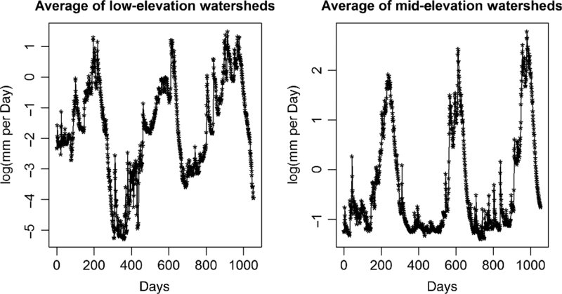
FIGURE 19.3 The different watersheds averaged.
For each watershed, a degree of fit within a watershed elevation group can be found by forming a regression of any one watershed against the average of the other three watershed values.
Analogously, for each watershed, a degree of fit between that watershed and the other elevation group can be found by forming a regression of that watershed against the average of all watersheds from the other group. This gives a rough numerical summary (R2) and graphical display of the within-group and between-group concordance or discordance. A complete numerical summary appears in Table 19.1 and a graphical display using Gregory Creek is also given (Figure 19.4).
TABLE 19.1 Preliminary Fit Measures Between and Within Groups (Fit to Original Scale, Based on the Model from Fitting a Simple Regression on the Filtered Scale)
| Watershed | Fit within elevation
groups R2pred, (R2) |
Fit between elevation
groups R2pred, (R2) |
| Low elevation | ||
| Gregory Creek | 0.8074
(0.8085) |
0.2200
(0.2224) |
| Rice Creek | 0.5267
(0.5289) |
0.3334
(0.3354) |
| Rock Creek | 0.6831
(0.6844) |
0.2842
(0.2866) |
| Baker Gulch | 0.6585
(0.6597) |
0.3139
(0.3159) |
| Mid elevation | ||
| Little Goose Creek | 0.7553
(0.7564) |
0.2291
(0.2324) |
| N Fork Slate Creek | 0.8302
(0.8307) |
0.4118
(0.4140) |
| Slate Creek | 0.8067
(0.8075) |
0.1702
(0.1730) |
| Boulder Creek | 0.7632
(0.7645) |
0.1902
(0.1933) |
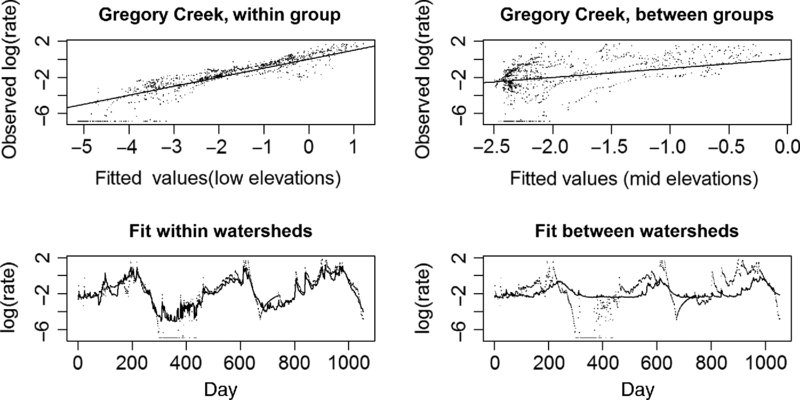
FIGURE 19.4 Using Gregory Creek as an example. The fit within a watershed and the fit between watersheds are compared (analysis on the filtered scale above, and original scale below).
It is not hard to see that the fitting within a watershed group is much better than the fit between groups. As can be seen from Figures 19.1, 19.2, and 19.3, the fact that the watershed elevation groups have different overall shapes makes it impossible for the average of the mid-elevation watersheds to fit Gregory Creek well, although the average of the other three watersheds within the elevation group produce a quite reasonable model for Gregory Creek.
19.4 RESULTS
It is quite obvious from a casual inspection of the data and preliminary graphs and computations that any analysis will show that the differences between groups are substantial compared to the differences within groups (exercises). Nevertheless, a definitive report of the findings should involve filtering the data and reporting the levels of R2pred on the original scale.
It is plain from a display of the relationships (Figure 19.4) that the fit within groups is much better than a fit between groups. In Figure 19.4, Gregory Creek is employed as an example. The fitted parameters are found using filtering, but the plots are of the data on the original scale. The upper graphs are the regressions and the lower graphs are the fitted values versus the observed values, over time. Numerical summaries save space and produce hard numbers. From Table 19.1, it is clear that the story is similar for all the watersheds.
Based on the results of Table 19.1, it is clear that every watershed fits (the average of) others within its elevation group far better than it fits the average of the other elevation group. Overall, the mid-elevation group seems to display more internal consistency than the low-elevation group, judging by the higher R2pred values within the group.
Paradoxically, North Fork Slate Creek has the distinction of having the highest correlation both to others within its group (0.8302) and to the average of the other groups (0.4118).
It is now time to ask the geoscience experts where they want to go next with this data.
EXERCISES
-
Perform a similar analysis comparing the high- and low-elevation groups.
- Fit a Fourier series to each watershed and find the estimated AR(m) order of the residuals.
- Plot the averaged watershed value for the high-elevation groups and discuss how this plot compares to the other watersheds. Is there any sense in which the shapes of the three groups form a natural progression from low to high elevations?
- Form a plot similar to Figure 19.4 using Frenchman Creek.
- Form a table as in the chapter, but comparing the low to the high elevations.
- Perform the analysis without filtering the data.
- Perform the analysis filtering the data [parts (iii) and (iv) will be different].
Observe that the patterns are the same in both tables (filtered and unfiltered), although the R2 values are consistently higher for the unfiltered analysis. Explain why this pattern occurs.