
20
VOSTOK ICE CORE DATA
20.1 SOURCE OF THE DATA
The Vostok ice core data is stored at the National Oceanic and Atmospheric Administration at these locations:
- ftp://ftp.ncdc.noaa.gov/pub/data/paleo/icecore/antarctica/vostok/deutnat.txt
- ftp://ftp.ncdc.noaa.gov/pub/data/paleo/icecore/antarctica/vostok/co2nat.txt. ftp://ftp.ncdc.noaa.gov/pub/data/paleo/icecore/antarctica/vostok/dustnat.txt
The original source (updated 11/2001) for this data is due to Petit et al. (1999).
The first file listed above contains a second column that is the estimated age of the reading and the last (fourth) column that is the temperature as deviations from a baseline level. The units for temperature are Celsius. A header in the original file explains each column in a lot more detail. Some of the first few rows of data in the file are presented in Table 20.1.
TABLE 20.1 Temperature Data (“Vostok temps.txt” in the Vostok Folder)
| Depth_corrected | Ice_age(GT4) | deut | deltaTS |
| 0 | 0 | −438 | 0.00 |
| 1 | 17 | −438 | 0.00 |
| 2 | 35 | −438 | 0.00 |
| … | |||
| 10 | 190 | −435.8 | 0.36 |
| 11 | 211 | −443.7 | −0.95 |
| 12 | 234 | −449.1 | −1.84 |
| 13 | 258 | −444.6 | −1.09 |
| 14 | 281 | −442.5 | −0.75, etc. |
This data is in the Vostok folder from the data disk and is denoted “Vostok temps.txt.” Obviously, the file must be brought into R using read.table() (with header = T), not scan().
The second files from NOAA contains the ice core CO2 measurements in ppmv (parts per million by volume). There are only two columns, the first is the estimated age and the second is the estimated CO2 level. The first few rows are presented in Table 20.2.
TABLE 20.2 CO2 Data (“Vostok CO2.txt” in the Vostok Folder)
| Gas_age | CO2 |
| 2342 | 284.7 |
| 3634 | 272.8 |
| 3833 | 268.1 |
| 6220 | 262.2 |
| 7327 | 254.6 |
| 8113 | 259.6, etc. |
These are obviously not direct measurements, and some investigation at the site would be required to determine the exact process whereby these values were estimated. Since this author does not have sufficient scientific background to assess the methodology by which changes in temperature, age, and/or CO2 levels were estimated, the numbers will be taken at face value here.
Ignoring the context of the problem, it would be hard for anyone to look at these graphs aligned in time (Figure 20.1) and not think there is something here requiring explanation.
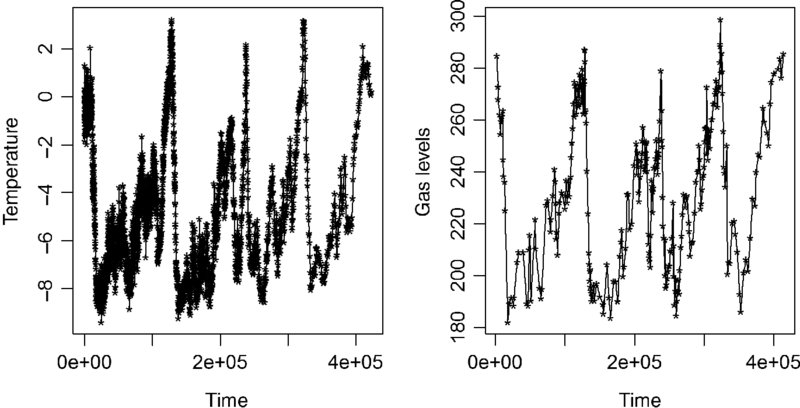
FIGURE 20.1 The parallels in these graphs are, of course, striking.
20.2 BACKGROUND
It has been noted that both CO2 levels and temperature have been rising in recent years. There is a strong association and a potential causal mechanism (the greenhouse effect). However, the relationship could be strong (CO2 drives temperature) or weak (the greenhouse effect could be minor and not the main reason for temperature change).
Perhaps the strongest counterargument to the climate change argument is that climate changes all of the time due to many, as yet poorly understood, causes. For example, there were a number of very cool periods (little ice ages), alternating with warming periods between 1550 and 1850 (see “Little Ice Age” in Wikipedia for extensive references).
The best evidence for countering this kind of criticism of a link between CO2 and temperature would be based on evidence showing a strong association over a very long time period (so long that long cycles of climate change could not be a highly plausible alternative explanation).
The Vostok ice core data goes back a little over 400,000 years. The data provides 283 measurements of CO2 and 3331 measurements of temperature change over this period. How strong is the association between CO2 levels and temperature change in this data? Using this data, is it possible to estimate the typical temperature change associated with a fixed increase in CO2 levels?
Disclaimer—please read before proceeding: Throughout this analysis the use of causal language will be avoided, not because of any skepticism about climate change, but because a single data set, based on an observational study, should never be used as the basis for a causal argument. The inference of cause–effect is a scientific pronouncement based on (i) all available evidence, (ii) the potential causal mechanisms, and (iii) the relative plausibility or implausibility of alternative explanations. In this regard, the video “The Question of Causation”(Against All Odds in the references), which follows the long line of evidence leading to the claim “smoking cause lung cancer”, would be worth viewing. This will be analyzed as a single data set; it is up to others to put all the evidence together. As a general practice, statisticians always avoid the use of causal language when discussing observational studies. Any assessment of causality in such cases is in the realm of subject-matter experts and not statisticians (or spin doctors).
20.3 ALIGNMENT
20.3.1 Need for Alignment, and Possible Issues Resulting from Alignment
The ice cores yield 3331 observations of changes in temperature, while the CO2 data yields 283 observations over the same roughly 400,000 years. In order to get a workable data set, the 283 CO2 observations must be matched with 283 of the 3331 temperature observations that match closely in time.
Alignment of the data was done manually by the author. It was based on finding close matches (in time) of the 3331 temperature values to the 283 CO2 values. Because two data sets have been aligned to produce a new data set, a number of questions needed to be addressed in order to continue with the analysis:
- Does the substantially reduced set of temperature data (283 vs. 3331 observations) still have the same basic pattern over, time, as the original data?
- Are the years for the CO2 and temperature data closely matched?
- To what degree are observations equally spaced? All the analyses we have done have been on equally spaced time series; this will no longer be the case (at least not exactly).
The aligned data is in the Vostok folder of the data disk and denoted as “aligned.txt.” The first few rows are given in Table 20.3. The degrees of match between columns 1 (the estimated time of the temperature measurement) and 3 (the estimated time of the CO2 measurement) is the first concern.
TABLE 20.3 The Aligned Data
| Ice_age | deltaT | Gas_age | CO2 |
| 2331 | −0.98 | 2342 | 284.7 |
| 3646 | 0.65 | 3634 | 272.8 |
| 3824 | −0.46 | 3833 | 268.1 |
| 6241 | 0.09 | 6220 | 262.2 |
| 7315 | −0.29 | 7327 | 254.6 |
| 8135 | 2.06 | 8113 | 259.6 |
| 10,124 | −0.58 | 10,123 | 261.6, etc. |
20.3.2 Is the Pattern in the Temperature Data Maintained?
To what extent this is to be expected and to what extent its sheer luck is unclear, but fortunately the subset of 283 observations seems to have kept the fundamental patterns in the data intact (Figure 20.2). In fact, many detailed features of the overall pattern are preserved in the subsample.
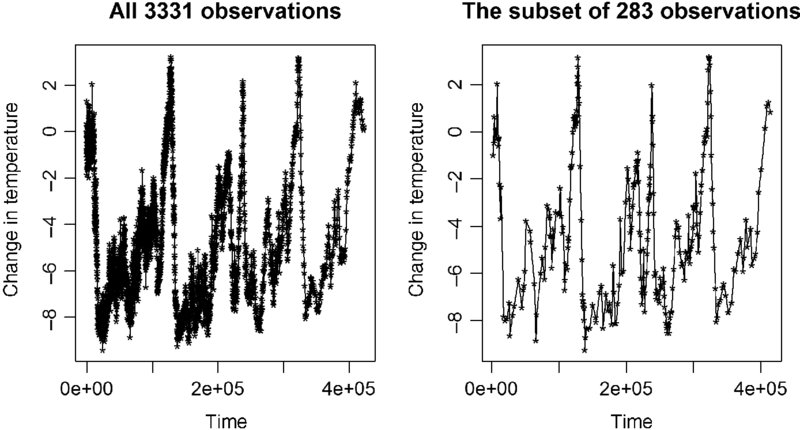
FIGURE 20.2 Is the temporal pattern preserved?
20.3.3 Are the Dates Closely Matched?
The times are well matched. The largest single difference was 317 years. About half the differences are less than 30 years. Given that the times span from about 2331 to 41,410, these are small differences. Based on the left panel of Figure 20.3, it would be hard to expect a better match between times than was found.
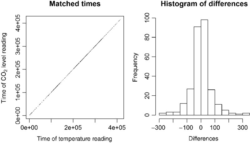
FIGURE 20.3 A scatterplot of time of CO2 reading versus time of related temperature reading, and a plot of the differences, in time, between related readings.
20.3.4 Are the Times Equally Spaced?
A variable, denoted “lag,” can be computed by taking differences between adjacent time periods. If this is done for the time stamps for the temperature data, the results are as follows summary(lag):
Min. 1st Qu. Median Mean 3rd Qu. Max.
55.0 665.8 1018.0 1460.0 1926.0 6012.0
Obviously, this will be the most significant challenge to analyzing this data as a time series. Two different analyses will be pursued. In the first approach, the data will be naively analyzed as if the spacing were equal. In the second analysis, an approach assuming an AR(1) model will be used. The AR(1) model can be generalized directly to unequal spacing. It should not be expected that either approach will be fully satisfactory, but both approaches should yield some insights into the data.
Figure 20.4 shows that there is no particular temporal pattern to the unequal spacing, in other words, large and small time lags are scatter throughout the entire time period.
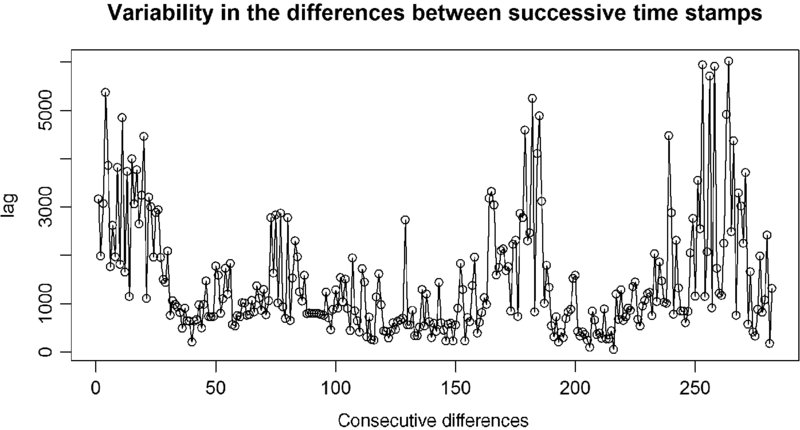
FIGURE 20.4 The differences between time stamps over time.
20.4 A NAÏVE ANALYSIS
20.4.1 A Saturated Model
The naïve analysis is quite straightforward. What could go wrong? In this model CO2 levels will be used to predict temperature. A cubic fit to the data will be chosen initially, although it would be nice to be able to reduce to a linear or quadratic model. The criteria R2F, pred will be used for model selection.
Because the CO2 values are quite large, a new variable, based on “CO2–mean (CO2),” (the mean is 234.0), will be used. This will prevent the squared and cubic terms in the regression from becoming excessively large and will reduce problems of co-linearity in the matrix of X values.
Fitting a cubic model, Figure 20.5, produces residuals that are AR(2).
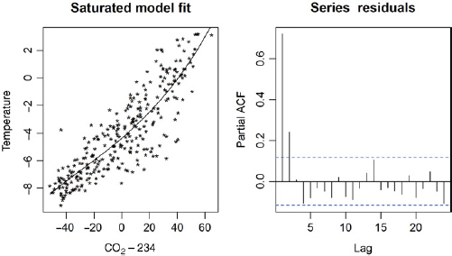
FIGURE 20.5 The initial saturated fit and residuals from the naïve (ignoring unequal spacing) analysis.
Furthermore, although AR(2) was selected, models of order 4 and 5 are very close in AIC value (Table 20.4). It may be wise to immediately adopt an AR(5) model to assure complete filtering.
TABLE 20.4 Several Models Fitted to the Residuals
| Order | ΔAIC | |
| 1 | 14.95 | 0.721 |
| 2 | 0.00 | 0.547, 0.241 |
| 3 | 1.98 | 0.545, 0.237, 0.008 |
| 4 | 0.70 | 0.546, 0.262, 0.067, –0.107 |
| 5 | 0.84 | 0.537, 0.267, 0.088, –0.063, –0.081 |
| 6 | 2.54 | 0.534, 0.265, 0.091, –0.054, –0.064, –0.033 |
As first discovered in Section 16.4.2.6, sometimes the data must be filtered twice. If an AR(2) model for the error were adopted here, this would be required. A way to avoid this, at least sometimes, is to foresee that a more complex model for the residuals looms on the horizon. The purpose of the filter is to get quasi-independent observations without giving up much sample size. The filter itself is of no intrinsic interest, nor is the order itself important. In this particular case, where the spacing is not even equal, it is particularly hard to attach any importance to the AR(m) model itself. In cases like this using a higher order filter, when the decision is close, is like washing with extra strength detergent.
Two key factors here are: (i) that the order 4 and 5 models are within one unit of the best model in terms of AIC differences, a very small difference, and (ii) the estimated values for ![]() are quite stable across all of these models (suggesting these more complex models really are refinements of, and not dramatically different from, the order 2 model).
are quite stable across all of these models (suggesting these more complex models really are refinements of, and not dramatically different from, the order 2 model).
20.4.2 Model Selection
After filtering once with an AR(5) filter, the resulting residuals are still AR(1) with ![]() . The second filter produces residuals not distinguishable from white noise [beginning with an AR(2) filter would have surely been even more convoluted].
. The second filter produces residuals not distinguishable from white noise [beginning with an AR(2) filter would have surely been even more convoluted].
Model selection information contained in Table 20.5 suggests that the linear model fits the data well, although not much better than the quadratic or cubic model. Because there is an interest in interpreting rates of change, it will be nice if a linear model holds up, suggesting a constant rate of change.
TABLE 20.5 Model Selection Table (![]() , SSTF= 342.25)
, SSTF= 342.25)
| Model | p | SSEF | R2F | R2F, pred | AICF |
| One mean | 1 | 342.25 | NA | NA | 1620.45 |
| Linear | 2 | 225.10 | 0.3423 | 0.3300a | 1506.38a |
| Quadratic | 3 | 225.05 | 0.3425 | 0.3213 | 1508.32 |
| Cubic | 4 | 222.85 | 0.3489 | 0.3192 | 1507.60 |
aBest model.
20.4.3 The Association Between CO2 and Temperature Change
From a summary of the best fitting filtered model, Table 20.6, it is trivial to determine that an increase of one unit in CO2 levels (ppmv) is associated with an increase of 0.059 in temperature (°C). The confidence interval is about a 0.0488 to 0.0684 increase in temperature (°C). It should be noted, before using the results from Table 20.6, that the residuals from the filtered analysis were assessed as white noise using ar.yw().
TABLE 20.6 Summary of the Best Fitting Model (with Filters A and A2)
| Coefficients: | ||||
| Estimate | SE | t-value | Pr(>|t|) | |
| A2 %*% (A %*% X) ones | −4.084623 | 0.249854 | −16.35 | <2e–16 |
| A2 %*% (A %*% X)new_CO2 | 0.058579 | 0.004896 | 11.96 | <2e–16 |
Although the relationship is not really strong, based on R2F, pred, the mesh between temperatures and CO2 levels is clear in the plot of “predictions versus time.” Recall the difference between the model fit over time and the complete prediction over time, is that the predictions use the fit and the previous 6 residuals [because the model for the noise is AR(6)], to produce an overall forecast for the next time period. The combined adjustment for the two filters can be extracted directly from the first row of the matrix A2%*%A, the resulting filtering matrix after application of each filter.
The quality of fit for both the fitted model and the predictions is given with a series of related R2-like values on the original scale.
The fit of the data to the model, after adjusting for AR(6) noise (Table 20.7), is quite strong (Figure 20.6). The relationship may or may not be causal, but it is certainly not likely to be coincidental.
TABLE 20.7 Fit Between the Data and the Model on the Original Scale
| Predictive model | R2 | R2pred |
| Fit alone | 0.6491 | 0.6432 |
| Fit with AR(6) adjustments | 0.9129 | 0.9117 |
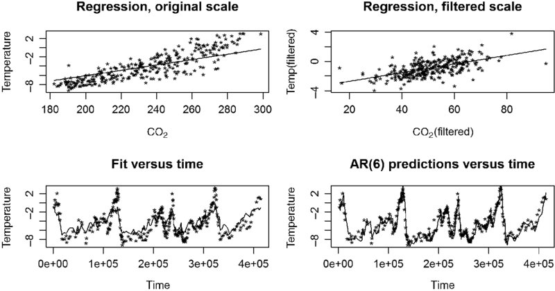
FIGURE 20.6 Displays for the naïve (ignoring unequal spacing) analysis of the Vostok data.
For the “fit alone” line, R2pred was found by combining the “hat” value from a linear fit on the original scale with the residuals from the model fitted on the filtered scale. These values were also used for the model with AR(m) adjustments, although it is not quite clear what “hat” values should be used in this case.
What follows in the rest of the chapter are attempts to “dig deeper” to assess both the reliability of this analysis and whether another analysis might yield better results. As a spoiler alert, there will not be much reason to either doubt or alter this analysis.
20.5 A RELATED SIMULATION
20.5.1 The Model and the Question of Interest
How might unequal spacing impact an analysis? Certainly this is a nebulous question, but a simulation meant to mimic this kind of data might offer some insights.
The following simulation will create data in much the way the Vostok data might be thought of as coming about and follow the same pattern analysis to get final results when it is known what the final result should be.
The scenario:
- An x variable varies over time.
- A model of the form y = β0 + β1x + ϵ.
- An MA(3) model for the errors (ϵ) with R2 ≈ 0.75.
- Create n = 1000 observations, but drop 71.7% of the observations at random.
The last step will create large gaps in the data producing data that is very unequally spaced in time. Three models will be compared: the true model, a model for all 1000 observations, and a model for the 283 observations left after dropping observations at random. The precise value of R2 is unlikely to matter, but the goal is to have a model that has both a clear signal and a clear noise. A simulation with n = 3200 is left as an exercise. Although a larger simulation is closer to modeling the actual Vostok data, the graphs are very noisy, so the smaller simulation is used for illustration and the larger simulation is left as an exercise.
The reason the question being addressed is nebulous, whether analysis of unequally spaced time series can get reasonable results using this naïve approach, is no one simulation could be conclusive and it is hard to list a set of scenarios that would satisfactorily answer the question. In an exercise, the student will be asked to produce a couple of other scenarios (with n = 3200). As with other simulations in this book, this example is illustrative rather than exhaustive.
20.5.2 Simulation Code in R
The data in Figure 20.7 was produced with the following code:
time <- c(1:1000)
# create a different model for different periods of time
x <- rep(NA,1000)
x[1:250] <- 3*cos(2*pi*(time[1:250]/80 +0.1))
x[251:500] <- 5*cos(2*pi*(time[251:500]/115 +.15))
x[501:750] <- 2*cos(2*pi*(time[501:750]/123))
x[751:1000] <- 3*cos(2*pi*(time[751:1000]/75 + .35))
# this is a model from 15.1.3, the standard deviation is altered by trial and error until the
# R2 value is about 0.75
error <- arima.sim(n = 1000, list(ma=c(0.8, 0.12, -0.144)), sd = 11.0)
y <- 3+10*x + error
fit <- lm(y ∼ x)
plot(time,y,pch=“*”)
lines(time,fit$fitted)
title(“The initial data”)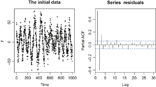
FIGURE 20.7 The original data for the simulation.
20.5.3 A Model Using all of the Simulated Data
The important things that were computed in the Vostok data were the confidence interval for the slope and the measures of fit and predictive accuracy on the original scale. The four-in-one graphs were also of value. All of these will be produced both for the full model and the model with just 283 observations. It is hoped the full analysis and the analysis with just 283 observations will be similar in these important ways.
The initial error structure appears quite complex, based on ar.yw():
  1      2      3       4       5       6       7      8
0.7896 -0.4765 0.1698 -0.0195 -0.0744 0.1478 -0.1085 0.0460
Order selected 8 sigma^2 estimated as 112
The filter produced residuals estimated to be white noise using ar.yw() on the first filtering. The parameter estimates are quite good:
 Coefficients:
             Estimate  Std. Error  t value  Pr(>|t|)
A %*% Xones  2.8659    0.6382      4.491     7.93e-06
A %*% Xx    10.3149    0.2558     40.329    < 2e-16
Using hypotheses tests as a reality check:
(2.8659 − 3.0)/0.6382 = −0.162 for the intercept and (10.3149 − 10)/0.2558 = 1.231. So the estimates match the parameters quite well (although the only direct interest is in the estimated slope, there would be some indirect concern if the estimate of the intercept were poor).
As usual, tracking and adjusting for AR(m) features in the residuals produce a better fit to the data (Table 20.8). As before, the “hat” values for the two models are found by fitting the model on original scale. The fit of the model to the data is displayed graphically in Figure 20.8.
TABLE 20.8 The Fit for the Filtered Model, the Original Scale, and the Original Scale with AR(8) Corrections
| Model | R2 | R2pred |
| Filtered | 0.6216 | 0.6201 |
| Fit, original scale | 0.7739 | 0.7730 |
| Fit with AR(8) adjustments | 0.8640 | 0.8612 |
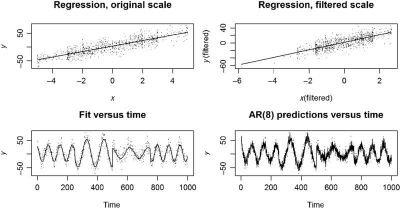
FIGURE 20.8 A four-in-one display of the fit to the simulated data.
20.5.4 A Model Using a Sample of 283 from the Simulated Data
Before examining a subset of the data, it is wise to anticipate what to expect. Comparing expectations to results is always more productive than just looking at results. It is hoped the slope is still estimated to be about 10.0, but the confidence interval should be wider.
It is hard to imagine what the filtering will be like, but it is expected that the R2-like values will drop across the board.
The following steps produce a random sample of 283 of the time periods:
new_time <- sample(time,283)
new_time <- sort(new_time)
The sample observations appear to retain the general pattern of the entire data (Figure 20.9). The sampling scheme did produce erratic spacing, but not as unusual as found in the Vostok data.
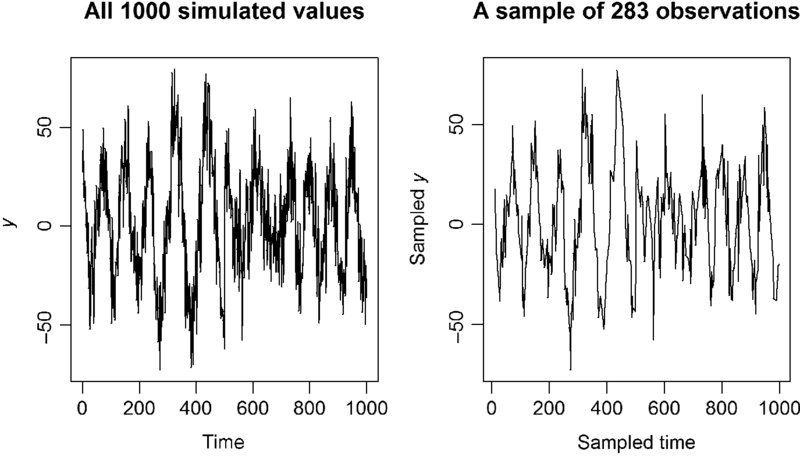
FIGURE 20.9 The subset of the original data still has much the same shape.
A variable “lag” was defined as lag <- new_time[2:283] - new_time[1:282]with results, summary(lag):
Min.  1st Qu.  Median  Mean  3rd Qu.  Max.
1.000  1.000  2.000   3.532  5.000  14.000
A total of 75 of the lags were equal to one.
The data, after fitting a regression as shown in Figure 20.10, where new_y is y[new_time], now appears to be AR(1)! 0.1798 , Order selected 1 sigma^2 estimated as 172.8. Of course, any subsampling is expected to reduce the order, m, of the AR(m) model (why?).
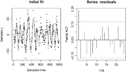
FIGURE 20.10 The initial fit to the data and the pacf() plot.
The filtered model has residuals identified as white noise based on ar.yw().
                 Estimate  Std. Error  t value  Pr(>|t|)
A %*% new_Xones  3.0378    0.9545      3.183    0.00162
A %*% new_Xnew_x 9.8493    0.3868     25.462    < 2e-16
The parameter estimates still seem reasonable. That is, (3.0378 − 3.0)/0.9545 = 0.0396 and (9.8493 − 10.0)/0.3868 = −0.390. Of course, the best way to assess this would be to fully automate the filtering process and perform this entire simulation perhaps 10,000 times and assess whether the results are as expected, in the long-run. The purpose of this section is more an exploration than a demonstration. As before, the filtered residuals are not much different from white noise based on ar.yw().
The model seems to fit the sampled data well (Figure 20.11). Because the corrected predictions only provide a small AR(1) correction, the fitted values and the predicted values are not much different.
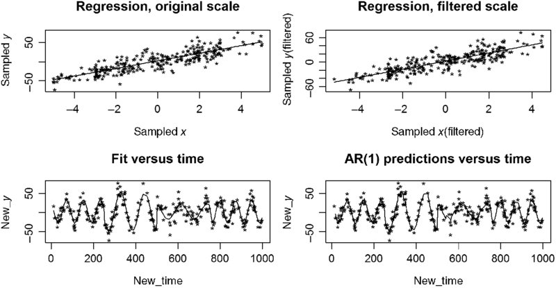
FIGURE 20.11 The fitted model using just n = 283.
The evidence from Table 20.9 is generally in agreement with Figure 20.11 that the filtering has become less effective. Comparing the fits to the full 1000 observations, there is less filtering [AR(8) vs. AR(1)], and while the filtered model has higher R2 values with the subset of the data, this does not translate to better fit on the original scale.
TABLE 20.9 Measures of Fit for the Subset of 283 Simulated Observations
| Model | R2 | R2pred |
| Filtered | 0.6984 | 0.6941 |
| Fit, original scale | 0.7638 | 0.7605 |
| Fit with AR(1) adjustments | 0.7715 | 0.7666 |
Compared to the full sample, this model has slightly lower R2 values on the original scale and these values do not improve nearly as much when adjustments are made to the residuals.
All of these results are good, considering the big picture. The implication is that, if a fuller set of data with equal spacing had been available, the confidence interval for the slope would have been narrower, and the R2 values would have been higher. Although any single simulation carries limited weight, it does lend some credence to the confidence interval for the slope given earlier (in the analysis of the actual Vostok data). All of these support, in a very limited way, that the results of the naïve analysis may well be fully reasonable.
20.6 AN AR(1) MODEL FOR IRREGULAR SPACING
20.6.1 Motivation
It has been established that, for the AR(1) model, the model can be “re-scaled” in the sense that ϵn = aϵn − 1 + wn implies, by iteration of the relationship, ![]() (Chapter 5). The skip method discussed in Section 13.7.2, for example, relies on the fact that, if equally spaced observations have an AR(1) error structure with coefficient a, then observations taken by skipping k observations apart will have an AR(1) structure with coefficient ak.
(Chapter 5). The skip method discussed in Section 13.7.2, for example, relies on the fact that, if equally spaced observations have an AR(1) error structure with coefficient a, then observations taken by skipping k observations apart will have an AR(1) structure with coefficient ak.
Modeling the error for one missing observation also reveals a pattern. Suppose the original errors are of the form: ϵ2 = aϵ1 + w2, ϵ3 = aϵ2 + w3, ϵ4 = aϵ3 + w4, ϵ5 = aϵ4 + w5, etc. However, if observation 3 is missing, the remaining errors could be modeled as: ϵ2 = aϵ1 + w2, ϵ3 missing, ϵ4 = a2ϵ2 + aw3 + w4, ϵ5 = aϵ4 + w5, etc. In other words, the model generalizes to an AR(1) model where the coefficient is aΔt, with a further caveat that the variance is greater when Δt is large (in an exercise you will show the ratio of the largest to smallest variance for data with missing values, when the original data had equal variance, is at most 1/[1 − a]).
Transitioning to a continuous model where the spacing is irregular, the model is ϵt = aΔtϵt − Δt + ωΔt, where ωΔt is a combination of previous and current white noise components.
Using this idea, the parameter a for an AR(1) model can be estimated by compensating for the unequal time lags. A filtering loop can be derived based on Δt and ![]() . This may or may not provide an effective filter, depending largely on whether the AR(1) model with constant a really does fit the data to some degree. In our data, the Δt's (lag_age) are quite large, we will find it is helpful, in solving the problem with the R function nls() to get manageable values. The normed value Δm = Δt/mean(Δt) will be used. Summary statistics for Δm in the Vostok data.
. This may or may not provide an effective filter, depending largely on whether the AR(1) model with constant a really does fit the data to some degree. In our data, the Δt's (lag_age) are quite large, we will find it is helpful, in solving the problem with the R function nls() to get manageable values. The normed value Δm = Δt/mean(Δt) will be used. Summary statistics for Δm in the Vostok data.
Min.     1st Qu.  Median   Mean     3rd Qu.   Max.
0.03356  0.45720  0.68480  1.00000  1.26800  4.11200
20.6.2 Method
The goal, then, is to find an optimal solution to the (nonlinear) least squares problem, when the parameter a is allowed to vary: ![]() Implemented in R this is
Implemented in R this is
fit_initial <- lm(temperature ∼ CO2 )
a_guess <- 0.5
next_residual <- fit_initial$residual[2:n]
previous_residual <- fit_initial$residual[1:(n-1)]
fit_a_nls <- nls(next_residual ∼ a^(delta_m)*previous_residual, start=list(a = a_guess))
The estimated value, ![]() , using this code is 0.74694. By trying several starting values, it is easy to see that the final estimate,
, using this code is 0.74694. By trying several starting values, it is easy to see that the final estimate, ![]() , is not dependent on the starting guess. The filtering can be handled using a “for” loop much more easily than a filtering matrix:
, is not dependent on the starting guess. The filtering can be handled using a “for” loop much more easily than a filtering matrix:
x_filtered <- rep(NA, 282)
y_filtered <- rep(NA, 282)
ones <- rep(NA,282)
CO2 <- CO2 - mean(CO2)	 # in the previous analysis this was done to control
# colinearity. This is done here also, so the outputs
# are comparable.
for(j in 1:282)
{ x_filtered[j] <- CO2[j+1] - .74694^(delta_m[j])*CO2[j]
ones[j] <- 1- 0.74694^(delta_m[j])
y_filtered[j] <- temperature[j+1] - 0.74694^(delta_m[j])*temperature[j]}
x_filtered <- cbind(ones,x_filtered)
fit_filtered <- lm(y_filtered ∼ -1+ x_filtered)
20.6.3 Results
The fitted model is summary(fit_filtered):
Coefficients:
            Estimate  Std. Error t value  Pr(>|t|)
ones       -4.510897  0.198124   -22.77   <2e-16
x_filtered  0.057020  0.004627    12.32    <2e-16
Although the parameter estimates are reasonable (compare to Table 20.6), the resulting residuals, diagnosed as AR(3) using ar.yw(), are not close to white noise.
Also the standard errors are (slightly) smaller than the previous analysis of Table 20.6, in other words they are probably too small. On the other hand, the mean square error for this model is 0.8373348 (summing the squared residuals and dividing by 280, the degrees of freedom) versus 0.7975, the estimated variance of a fully filtered model [also from ar.yw() applied to these residuals].
A second filtering, assuming equal spacing, produces nearly identical results to the first approach, with residuals not distinguishable from white noise, based on ar.yw():
Coefficients:
                    Estimate  Std. Error  t value Pr(>|t|)
A2 %*% Xones        -4.529512 0.250955   -18.05   <2e-16
A2 %*% Xx_filtered   0.050532 0.004916    10.28   <2e-16
MSE for this model being 0.77606.
Overall, this approach seems to support the previous analysis. In other words, this approach, followed up with a second AR(3) filter, got results similar to the first analysis. This analysis, while it did not fully succeed, would seem to be less dependent on the equal spacing assumption.
Usually, when two different, reasonable analyses yield nearly identical results for a set of data, the suggestion is that “All roads lead to Rome”, and any reasonable analysis would produce the same result.
20.6.4 Sensitivity Analysis
Nevertheless, because this data is relatively famous (or infamous in some circles) and because both analyses made use of some key assumptions not met (the first analysis assumed equal spacing, which is certainly not close to being true; the second analysis assumed an AR(1) model and needed to use the assumptions of equal spacing for the second, admittedly, minor filtering), the data will be further prodded and poked without much additional insight.
It is possible that the model is AR(1), but that the value of a changes over the course of time. In any case, something could be learned from fitting the model over different subsets of the data. Dividing the data into four segments of roughly 70 data point, the filtered regressions were run after using nls() to get a different ![]() for each period.
for each period.
The analysis with varying time periods (Table 20.10) suggests the value of a does vary over time, but that even reducing the time periods to about 100,000 years allows, half the time, for an AR(1) model to filter the data such that the residuals cannot be distinguished from white noise using ar.yw(). Although there is variation in the parameter estimates, value similar to the previous two analyses is found.
TABLE 20.10 Analysis over Different Time Periods
| Model | n | Order of
residuals |
|||
| 10,151.1 years
(2336.5–12,487.6) |
71 | 0.6853
(0.088) |
–4.13
(0.396) |
0.060
(0.0107) |
0 |
| 93,935.5 years
(12,575.5–219,709) |
70 | 0.522
(0.125) |
–4.45
(0.25) |
0.0898
(0.0082) |
0 |
| 72,307.5 years
(220,174.5–292,482) |
72 | 0.7305
(0.1007) |
–5.48
(0.43) |
0.0479
(0.0097) |
2 |
| 120,388.5 years
(293,727.5–414,116) |
70 | 0.7975
(0.0784) |
–3.51
(0.42) |
0.0481
(0.0086) |
2 |
Parameter estimates are given with standard errors in parentheses on the next line.
20.6.5 A Final Analysis, Well Not Quite
The technique of moving windows could be used to estimate a(t), the AR(1) parameter as a function of time. The data could then be filtered based on both the estimate ![]() and the spacings Δt.
and the spacings Δt.
It is possible to use moving windows to estimate a locally, but the nls() function experiences failure to converge for windows less than 47. Because of a desire to get highly variable local estimates, this window was used (the usual tradeoffs between bias and variance are at work in choosing a window here). Figure 20.12 shows the values of ![]() for the narrowed possible window (w = 47) and a very wide window (w = 95).
for the narrowed possible window (w = 47) and a very wide window (w = 95).
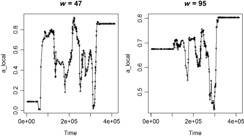
FIGURE 20.12 The local value of  is obviously smoother for a wider window.
These models produce regressions similar to those already discussed, but still with residuals that are not white noise. It is worth examining the residuals more closely.
Figure 20.13 shows that locally the order of the residuals can be anywhere from order 0 to order 6 as diagnosed using ar.yw(), although the usual caveat that the ar.yw() function assumes equal spacing.
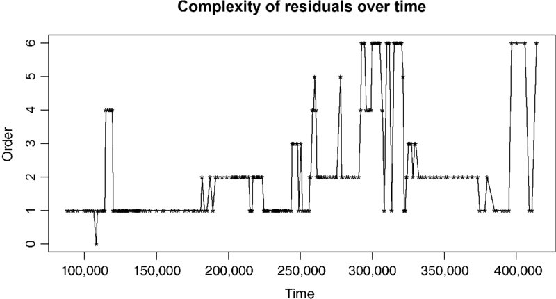
FIGURE 20.13 Local clusters of residuals, taken 40 at a time, with ar.yw() used to diagnose order, can have an order as high as 6.
It seems clear that none of the models considered in this last effort, assuming AR(1) errors, fully solve the problem of unequal spacing. However, a model for a more complex model, AR(2) or higher, with extremely unequal spacing is well beyond the scopes both of this book and the author's competence.
Nevertheless, the analyses provided here, which are substantial improvements on any method that ignores serial correlation, do produce relatively consistent results suggesting an increase of CO2 of about 10 ppm would be associated with (this language is commonly used in the regression literature and is explicitly meant to avoid coming down on either side of the question of causation) an increase in temperature of about 0.5°C.
20.7 SUMMARY
A naïve analysis of the data, applying the modeling efforts from previous chapters while ignoring the unequal spacing of the observations produced an “acceptable” result. The result was acceptable in the sense that the filtering mechanism developed was successful in producing quasi-independent observations, the goal of filtering, even though the conditions assumed in developing the filter were not met.
A second simulation analysis suggested that this might not be an accident. In a simulation producing data with unequal spacing, it was found that the filtering can indeed work and the resulting statistical analysis seemed to match the model that produced that data.
Finally, another approach was explored that turned out to be a partial dead end, at least in this case. It was assumed that the data was AR(1) and a model was fit that allowed for varied spacing between observations. While this approach did not fully filter the data, a final AR(1) filter applied to the resulting filtered values produced a model similar to the naïve analysis.
However, further examination shows that an AR(1) is probably always going to look promising, but never quite solve the problem. This could be viewed as homage to all the dead ends that were explored in this book that ended up in the wastebasket, as well as all the dead ends consulting statisticians, researchers, and graduate students go down every day. Science only appears in the final publications and other final results. Behind every good result are a lot of full recycling bins. Certainly this was the most interesting dead end explored in the course of writing this book.
EXERCISES
-
Filter the Vostok cubic regression with an initial AR(2) model, the one suggested by ar.yw(), and find the order of the residuals after filtering.
-
Show that ar.mle() and ar.yw() provide similar analysis for the residuals from the cubic Vostok model, both in the choice of model and in which models are considered close to the best models based on AIC values.
-
In the text, the time stamps for the temperature data were explored to determine the degree of equal or unequal spacing. Compute a “lag” variable for the CO2 time stamp and perform a similar analysis. How does this compare to the “lag” for the temperature time stamp. Explain why this result is not surprising.
-
Show that, if a model is AR(1) with constant variance and gaps appear in equally spaced data, the ratio of the largest variance to the smallest variance is at most 1/[1 − a].
-
A students argues: “It doesn't matter where the filter (A) came from, if the result is quasi-independent observations [observations not distinguishable from white noise based on ar.yw() or ar.mle()], then the assumptions of the regression model are met.” Comment on this claim.
-
In the book the phrase “residuals not distinguishable from white noise” is used a lot. Why would it be less correct to say “residuals that are white noise.”
-
Develop a simulation similar to the one in Section 20.5 with 0.65 < R2 < 0.85. Use the ARMA(m,l) structure below and pick your own parameters for the periodic functions.
- Simulate the data with n = 3200.
- Perform a hypothesis test for the slope coefficient, based on a filtered model.
- Form a random sample of 283 observations from the original 3200.
- Perform a hypothesis test for the slope coefficient, based on a filtered model.
Your class results can be pooled to get an overall assessment of the reliability of filtering in this context.
ARMA(m,l) structures:
- (1 − 0.7B)(1 + 0.1B)ϵn = (1 − [0.4 + 0.4i]B)(1 − [0.4 − 0.4i]B)wn
- (1 − [0.7 + 0.1i]B)(1 − [0.7 − 0.1]B)ϵn = (1 − 0.6B)(1 − 0.3B)wn